Why Do Granular Materials Stiffen with Shear Rate? A Test of Novel Stress-Based Statistics

Abstract

Recent experiments exhibit a rate-dependence for granular shear such that the stress grows linearly in the logarithm of the shear rate, $\dot{\gamma}$. Assuming a generalized activated process mechanism, we show that these observations are consistent with a recent proposal for a stress-based statistical ensemble. By contrast, predictions for rate-dependence using conventional energy-based statistical mechanics to describe activated processes, predicts a rate dependence that of $(\ln(\dot{\gamma}))^{1/2}$.

-

Understanding disordered solids, such as foams, glasses, polymers, colloids and granular materials is a great challenge for statistical physics. Several of these systems, including granular materials, fall outside the rubric of conventional statistical mechanics because they are dissipative. But, these materials exhibit well defined statistical distributions. Several novel approaches have been recently proposedEdwards and Oakeshott (1989); Makse and Kurchan (2002); Ono et al. (2002); O’Hern et al. (2005); Snoeijer et al. (2004); Tighe et al. (2005); Henkes and Chakraborty (2005); Henkes et al. (2007) to characterize the statistics of these dissipative materials,. We focus on testing one of the proposed statistical frameworks, the force or stress-based ensemblesSnoeijer et al. (2004); Tighe et al. (2005); Henkes and Chakraborty (2005); Henkes et al. (2007), and specifically the stressed-based ensemble hypothesized by SH and BCHenkes and Chakraborty (2005); Henkes et al. (2007) to account for the coupling between forces and geometry. Here, we test this hypothesis by showing that it can account for experimentally observed logarithmic strengthening with increasing shear rate in slowly sheared granular systems. Many models of slow, dense granular flows assume that the internal stresses are independent of shear rate. Linear rate-dependence for shear stresses occurs for Newtonian fluids. Non-linear dependence on rate is common in non-Newtonian fluids, as well as in the “glassy” systems noted aboveSollich et al. (1997); Sollich (1998). The stress-based ensemble offers an explicit framework for analyzing the rheology of such non-thermal, glassy systems.

Recent 2D Hartley and Behringer (2003) and 3DDaniels and Behringer (2005) experiments on sheared dense granular materials, showed mean stresses that grow linearly with $\ln(\dot{\gamma})$, where $\dot{\gamma}$ is the shear rate. Indeed, rate-dependence spans many decades in $\dot{\gamma}$, as seen in Fig. 1, which show time-averaged stresses acquired in a 2D Couette shear experiment that is sketched in Fig. 1. Fig. 2 shows typical traces of stress vs. time for several different shear rates, $\dot{\gamma}$. These data have also been acquired for various packing fractions, $\phi$, relatively near the critical packing fraction, $\phi_{c}$, below which the system is unjammedO’Hern et al. (2002); Howell et al. (1999) and shearing stops.

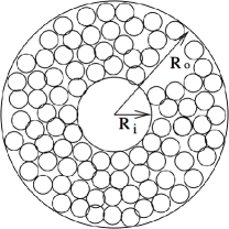
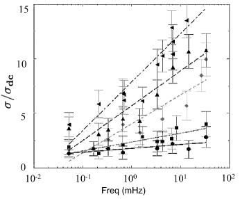
Figure 1: Top, sketch of Couette shear apparatus, not to scale. $R_{o}=19.2\,cm$. Data is for small/medium shearing wheels, where $R_{i}=6.7\,cm/5.3\,cm$. Particles are either circular or pentagonal in cross section, and have dimensions between $0.7\,cm$ and $0.9\,cm$. Bottom: Data for the mean stress in a segment of a 2D granular Couette experiment containing roughly 200 particles vs. shear $\dot{\gamma}$. Data (normalized by $\rm\sigma_{dc}\simeq 4.11Nm^{-1}$) are for different packing fractions $\phi$ relative to the critical packing fraction, $\phi_{c}$, where stesses fall to zero. Symbols are: circles: $\phi-\phi_{c}=0.0012$, squares: $\phi-\phi_{c}=0.0091$, diamonds: $\phi-\phi_{c}=0.0152$, upward pointing triangles: $\phi-\phi_{c}=0.0189$, left-pointing triangles: circles: $\phi-\phi_{c}=0.0226$. We also consider other data (below) from experiments by Hartley and BehringerHartley and Behringer (2003).

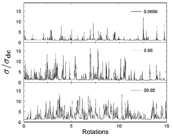
Figure 2: Time series for different $\dot{\gamma}$ (in mHz) for the stress, for the smaller $R_{i}$ above.

We construct a model for the behavior of the force fluctuations seen in the Couette shear experiments. The first model premise is that the shearing process causes build-up of inhomogeneous stress structures, such as force chains, which fail when they reach a critical yield stress. A blow-up of a typical time series for the stress in Fig. 3 gives a good flavor of this process.

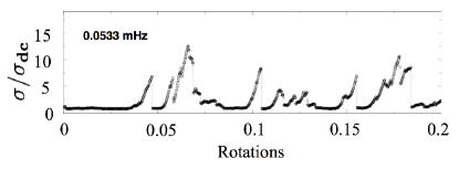
Figure 3: Blow up of time series data for the stress at $\dot{\gamma}=0.0533mHz$ showing stress fluctuations over 0.2 rotations of the inner shearing wheel. The data indicate the approximately linear loading up of force structures and their more rapid failure.

The actual failure process is complex except very near jamming ($\phi\simeq\phi_{c}$), where there are typically only one or two visible force chains in an observation region. More generally, for $\phi$ much larger than $\phi_{c}$, there is a (strong) force network, and when a stress drop occurs, it is typically concentrated on a subset of grains on a more or less linear region of the force network, often extending for many grains. The stress drop is very fast relative to the build-up, indicating a failure of part of the network, while much of the remaining network is only weakly affected. We use the common term “force chains” to refer to segments of the strong force network that exhibit the force build-up and failure process that is the fundamental origin of granular force fluctuations, but we do not consider the specific origins of the failures (e.g. shear-transformation-zone eventsLemaitre (2002), force chain bucklingTordesillas et al. (2008), etc.). Rather, we explore the role played by the background of force fluctuations generated during the build-up and failure process. We ask whether the effect of these fluctuations can be described in terms of a stress-based ensemble. And we exploit the fact that force changes following failure are localized to force chains, with a much weaker effect on the rest of the system.

We expect that a chain will fail if the force/stress on it, $\sigma$, exceeds a characteristic value $\sigma_{m}$. This is reminiscent of Coulomb failure, but refers to failures of localized structures, with no strict frictional analogy. We begin by considering a single event consisting of the birth-to-death cycle of a single force chain, relevant to systems with $\phi\simeq\phi_{c}$, and then return to an accounting for multiple events occuring in a given observation region for packings with $\phi>>\phi_{c}$.

A key premise of the model is that the failure is an activated process aided by stress fluctuations, similar to a thermally activated escape from a potential well. The potential well is replaced by a stress trap that models the meso-scale strong force network, and chain failures correspond to escape from a trap. The fluctuations of thermal equilibrium are replaced by fluctuations of stress in the network, characterized by a temperature-like quantityHenkes et al. (2007). These fluctuations occur as the granular assembly moves through a series of states at mechanical equilibrium. For thermally activated processes, the rate of escape is proportional to $e^{-\beta E_{barrier}}$, where $\beta=(k_{B}T)^{-1}$ is the inverse temperature and $E_{barrier}$ is the barrier height. To construct a framework for activated dynamics in systems where the fluctuations are athermal stress fluctuations, we appeal to a recently-developed statistical framework for granular assembliesHenkes and Chakraborty (2005); Henkes et al. (2007). In this framework, the ensemble of mechanically stable states is defined by a Boltzman-like probability distribution:

$$P_{\nu}=(1/Z)e^{-\alpha\Gamma_{\nu}}~{},$$ (1)

where $\Gamma_{\nu}=S_{\nu}\sigma_{\nu}$ is an extensive quantity related to the stress of the configuration $\nu$, and $S_{\nu}$ is the area occupied by the grainsHenkes and Chakraborty (2005); Henkes et al. (2007). In Eq. 1, $\alpha$ is the analog of the inverse temperature, $\beta$, and characterizes the fluctuations. In analogy with thermally activated processes, the probability per unit time of chain failure is then given by

$$P_{f}=A\exp[-\alpha\Gamma_{barrier}].$$ (2)

Assuming that the area fluctuations are small compared to the stress fluctuations (the area is fixed in the experiments discussed above), the effective barrier to be surmounted by a force chain with a stress $\sigma$ on it becomes $\Gamma_{{barrier}}=S(\sigma_{m}-\sigma)$, and the failure rate (per unit time) is:

$$P_{f}=A\exp[-(\sigma_{m}-\sigma)/\sigma_{o})].$$ (3)

We have used $\sigma_{0}$ to denote $1/(\alpha S)$.

Both $A$, the attempt frequency, and $\sigma_{o}$ may depend on $\dot{\gamma}$, but to lowest order, we will treat these as constants. We expect that the stress on a force chain increases linearly in time until a chain fails (e.g. Fig. 3). Thus,

$$\sigma=\sigma^{\prime}t={\Sigma}{\dot{\gamma}}t,$$ (4)

where ${\Sigma}$ is a measure of rate of stress increase per unit shear deformation, which we also assume is a constant. With this picture, the force chain loads up steadily in time, but the probability of failure depends on the closeness of $\sigma$ to $\sigma_{m}$. If $\sigma<<\sigma_{m}$, the probability of failure/unit-time should be low, but as $\sigma$ approaches $\sigma_{m}$, the probability of failure should become large. A range of parameters where the process is strongly activated is $A<<\dot{\gamma}$, and $\sigma_{m}>>\sigma_{o}$, the analog of the low-temperature limit of a thermally activated process. This limit likely applies to the experiments since the time-dependence of the stress is dominated by slow build up and rapid release. This is the regime we focus on in this work. The assumption of strongly activated behavior is also consistent with the fact that the experiments suggest logarithmic rate dependence over many decades of $\dot{\gamma}$, without a crossover to different behavior at low $\dot{\gamma}$.

We treat the loading up of the networks in a probabilistic manner. If the probability for the chain to survive until time $t$ without failing is $P_{s}(t)$, then

$$P_{s}(t+dt)=P_{s}(t)(1-P_{f}(t)dt),$$ (5)

or

$$P_{s}^{-1}dP_{s}/dt=-P_{f}.$$ (6)

We first consider the idealized situation of isolated chains, so that we need only consider one such chain at any given instant, and focus on the evolution of stresses from the formation of the chain to its failure. The time average moments of $\sigma$ are:

$$\bar{\sigma^{n}} = (1/T)\int_{0}^{T}dt(\sigma(t))^{n}$$ (7)

$$= \int d\tau P_{s}(\tau)P_{f}(\tau)\int_{0}^{\tau}dt(\sigma(t))^{n}/\int d\tau P_{s}(\tau)P_{f}(\tau)\tau$$

where we have used, $T=\int d\tau P_{s}(\tau)P_{f}(\tau)\tau$. Defining $\langle\sigma^{n}\rangle=\int d\tau P_{s}(\tau)P_{f}(\tau)(\sigma(\tau))^{n}$, we can write $\bar{\sigma}^{n}=\langle\sigma^{n+1}\rangle/((n+1)\langle\sigma\rangle)$ The above equation reflects an ensemble average over chains surviving up to time $\tau$ and failing within $\tau$ to $\tau+d\tau$, with probability $P_{s}(\tau)P_{f}(\tau)$. We can use Eq. 6 to write:

$$\langle\sigma^{n}\rangle=-\int(\sigma(\tau))^{n}(dP_{s}/d\tau)d\tau$$ (8)

Introducing the dimensionless time, $\theta=\dot{\gamma}\tau$, we can write

$$d\ln(P_{s})/d\theta=-B\exp({\Sigma}\theta/\sigma_{o}),$$ (9)

where we we have absorbed some of the constants into a single expression $B=(A/\dot{\gamma})\exp(-\sigma_{m}/\sigma_{o})$. Integrating Eq. 9, using $P_{s}(0)=1$, and integrating Eq. 8 by parts, we can write $\langle\sigma^{n}\rangle$ as:

$$\langle\sigma^{n}\rangle=n{\Sigma}^{n}\int{\theta}^{n-1}\exp[(B/p)(1-\exp(p\theta))]d\theta$$ (10)

Here we define $p={\Sigma}/\sigma_{o}$. In the special case $n=1$, it is possible to relate this integral to known functionsAbramowitz and I. A. Stegun (1972), but this does not appear to be true for the general case, and it is now convenient to introduce a dimensionless rate, $s=p/B$:

$$s=(\dot{\gamma}{\Sigma})\exp(\sigma_{m}/\sigma_{o})/(A\sigma_{o})$$ (11)

Differentiating $\langle\sigma^{n}\rangle$ with respect to $s$ yields, after a bit of algebra:

$$sd\langle\sigma^{n}\rangle/ds=-\langle\sigma^{n}\rangle/s+n\sigma_{o}\langle\sigma^{n-1}\rangle.$$ (12)

To calculate the time-averaged stress $\bar{\sigma}$, we need to calculate $\langle\sigma\rangle$ and $\langle\sigma^{2}\rangle$. The average $\langle\sigma\rangle$,

$$d\langle\sigma\rangle/ds=-\langle\sigma\rangle/s^{2}+\sigma_{o}/s.$$ (13)

We are concerned with the strongly activated regime of $A<<\dot{\gamma}$ and $\sigma_{m}>>\sigma_{0}$, $s>>1$, which justifies an expansion involving $s$ and its logs. In lowest order when $s<<1$:

$$\langle\sigma\rangle\simeq\sigma_{o}\ln(s)+C$$ (14)

or

$$\langle\sigma\rangle=\sigma_{m}+\sigma_{o}\ln({\Sigma}/\sigma_{o})+\sigma_{o}\ln(\dot{\gamma}/A)+C_{1},$$ (15)

where $C_{1}$ is a constant of integration. Similarly, keeping the leading terms in $s$, the expression for $\langle\sigma^{2}\rangle$ is:

$$d\langle\sigma^{2}\rangle/ds \simeq 2\sigma_{0}\langle\sigma\rangle/s$$

$$\langle\sigma^{2}\rangle = \sigma_{0}^{2}(\ln s)^{2}+C_{2}$$ (16)

where $C_{2}$ is another integration constant. Assuming the integration constants are much smaller than $\ln(s))$,

$$\bar{\sigma}={{\langle\sigma^{2}\rangle}\over{\langle\sigma\rangle}}\simeq\sigma_{0}\ln s$$ (17)

In fact, we can now see if omitting the term $-\langle\sigma\rangle/s^{2}$ at lowest order is self consistent. We estimate $\langle\sigma\rangle\simeq\sigma_{m}$, and then obtain a ratio of the two terms on the right side of Eq. 13:

$$[\langle\sigma\rangle/s^{2}]/[{\Sigma}/(sp)]\simeq(\sigma_{m}/{\Sigma})(A/\dot{\gamma})\exp(-\sigma_{m}/\sigma_{o}).$$ (18)

Indeed, this ratio should be small, so the dominant rate effect on the mean stress should be a logarithmic stengthening.

We now turn to how the mean–i.e. long-time averaged stresses from the whole network within a measurement domain would be manifested in a continuous shear experiment. For instance, in the 2D Couette experimentsHartley and Behringer (2003), time-dependent force data are obtained in a finite region comprising roughly 10% of the whole system. In 3D experimentsDaniels and Behringer (2005), pressure measurements are made over an area which contacts several tens of particles. In both cases, the mean stress is computed as a time average. Here, we focus on the 2D experiment, since it has yielded data over a range of densities. If $\phi$ were such that on average only one force chain existed at a time, then our analysis so far would yield the mean stress. However, in general, it is necessary to adjust this result for the mean number of chains (or failure events), $N(\phi)$, that are generated per unit time interval or angular displacement in the region of interest. Note that to lowest order, this is simply a function of $\phi$. In principle, we can determine this quantity and hence $\sigma_{o}$ in order to compare to preditions from the stress ensembleHenkes and Chakraborty (2005); Henkes et al. (2007). For instance, from recent experiments by Sperl et al. on the same 2D Couette systemSperl et al. (2008), we estimate (at fixed $\dot{\gamma}$) that $N(\phi)\propto(\phi-\phi_{c})^{a}$ and $\sigma\propto((\phi-\phi_{c})^{b}$, where $a\simeq 2$ and $b\simeq 1$. Data from Hartley et al.Hartley and Behringer (2003), such as Fig. 1, yield $N(\phi)\sigma_{o}$ by taking the slope of $\sigma/\sigma_{DC}$ vs. $\ln(\dot{\gamma})$. Unfortunately, the current data is not sufficiently precise to give a good determination of $\sigma_{o}$ by this process.

Nevetheless, Eq.18, with the above $\phi$-dependent corrections, makes a prediction, the key result of this work: $\bar{\sigma}\propto\ln(\dot{\gamma})$, with a proportionality constant of $\sigma_{o}$, multiplied by $N(\phi)$. Qualitatively, the strengthening of the material with shear rate occurs because the failure probability per unit time for a given $(\sigma_{m}-\sigma)/\sigma_{o}$ is independent of $\dot{\gamma}$ whereas the buildup of stress grows linearly with $\dot{\gamma}$. There is, therefore, a competition between the stress buildup and the failure process. If the failure rate were independent of $\sigma$ (large $\sigma_{0}$ limit), then, it follows from Eq. (4) that the average stress would grow linearly with the shear rate, as in Newtonian fluids. In the opposite limit of failure occurring only if the force chains are loaded up to $\sigma_{m}$ ($\sigma_{0}\rightarrow 0$ limit), there would be a fixed time $\propto 1/\dot{\gamma}$ between failures and the average stress would become independent of the shear rate. The exponential increase of the failure rate with $\sigma$ leads to the logarithmic strengthening. Interestingly, Eq. 12 indicates a much weaker rate dependence for the variance, $V=\langle\sigma^{2}\rangle-(\langle\sigma\rangle)^{2}$: $dV/ds=(-V+(\langle\sigma\rangle)^{2})/s^{2}$.

The distribution of the stress drops, $\Delta\sigma$, occuring for each “avalanche” in a time series is sensitive to the distribution of $\sigma_{m}$, and this distribution can be calculated exactlySollich (1998); Bi et al. (2008) for an experimentally realisticGeng and Behringer (2005) exponential distribution of $\sigma_{m}$: $e^{-\sigma_{m}/\sigma_{m}^{0}}$. For $\Sigma\dot{\gamma}/\sigma_{0}<<A(e^{\Delta\sigma/\sigma_{0}}-1)$, the distribution is

$$P(\Delta\sigma)=e^{\Delta\sigma/\sigma_{0}}\big{[}{1\over{e^{\Delta\sigma/\sigma_{0}}-1}}\big{]}^{(1+\sigma_{0}/\sigma_{m}^{0})}~{},$$ (19)

which we have fitted to the experimental data for stress drops, ensuring that the chosen data meet the criterion for which Eq. 19 is applicable. Representative data at $\phi-\phi_{c}=0.01373$ are shown in Fig. 4. The ratio of the two fitting parameters, $\sigma_{0}/\sigma_{m}^{0}$, follows by fitting the exponent of the power law regime, and $\sigma_{m}^{0}$ can be estimated from a fit to the exponential tail. We use these values to constrain the fitting to the full form of Eq. 19.

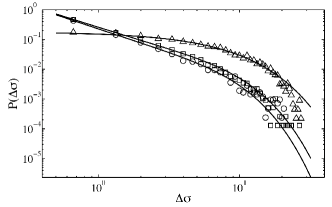
Figure 4: Fits (solid lines) to Eq. 19 of experimental data for $\Delta\sigma$ at $\phi-\phi_{c}=0.01373$, and $\dot{\gamma}$’s of 0.066 mHz (circle), 0.6645 mHz (square) and 13.307 mHz (triangle). The fits yield $\sigma_{0}\simeq 2.0$, independent of $\dot{\gamma}$ and $\sigma_{m}^{0}/\sigma_{0}\simeq 1.58~{},1.82~{},2.0$ (lowest to the highest value of $\dot{\gamma}$.)

The analysis presented in this letter is reminiscent of the soft glassy rheology (SGR) modelSollich et al. (1997); Sollich (1998) with the important distinction that the role of energy is being played by the stress. The noise temperature $x$ of the SGR is replaced by $1/\alpha$ in the stress-based ensemble. The SGR model incorporates disorder through a distribution of activation barriers, which in the context of the current work would translate to a distribution of $\sigma_{m}$. The average stress is not sensitive to the distribution of $\sigma_{m}$ in the large $s$ limit, and scales as $(\ln{\dot{\gamma}})$. The difference with the SGR result, $(x\ln{\dot{\gamma}})^{1/2}$, can be explained through replacement of an energy barrier by a stress barrierBi et al. (2008).

The present analysis is a first step towards understanding linear logarithmic strengthening in granular materials which distinguishes granular rheology, with dissipative interactions, from that of other materials. A key point is that a stress ensemble rather than a energy ensemble yields the correct rate scaling. Force networks are visually obvious in the experiments, but their quantitative connection to the complete stress states has not yet established. Characterization of mesoscale structures such as force networks, and their connection to macroscopic variables such as stress remains a great challenge for the field. Adopting the framework of the SGR model with its meanfield approach to correlations but with the noise temperature and energy replaced by their counterparts from the stress-based ensemble should provide a fruitful avenue for building these connections.

This work was supported by NSF-DMR0555431, the US-Israel Binational Science Foundation #2004391, and, NSF-DMR0549762.

References

- Edwards and Oakeshott (1989) S. F. Edwards and R. B. S. Oakeshott, Physica D 38, 88 (1989).
- Makse and Kurchan (2002) H. A. Makse and J. Kurchan, Nature 415, 614 (2002).
- Ono et al. (2002) I. K. Ono, C. S. O’Hern, D. J. Durian, S. A. Langer, A. J. Liu, and S. R. Nagel, Phys. Rev. Lett. 89, 095703 (2002).
- O’Hern et al. (2005) C. S. O’Hern, A. J. Liu, and S. R. Nagel, Phys. Rev. Lett. 93, 165702 (2005).
- Snoeijer et al. (2004) J. H. Snoeijer, T. J. H. Vlugt, M. van Hecke, and W. van Saarloos, Phys. Rev. Lett. 92, 054302 (2004).
- Tighe et al. (2005) B. P. Tighe, J. E. S. Socolar, D. G. Schaeffer, W. G. Mitchener, and M. L. Huber, Phys. Rev. E 72, 031306 (2005).
- Henkes and Chakraborty (2005) S. Henkes and B. Chakraborty, Phys. Rev. Lett. 95, 198002 (2005).
- Henkes et al. (2007) S. Henkes, C. S. O’Hern, and B. Chakraborty, Phys. Rev. Lett. 99, 038002 (2007).
- Sollich et al. (1997) P. Sollich, F. Lequeux, P. Hebraud, and M. E. Cates, Phys. Rev. Lett. 78, 2020 (1997).
- Sollich (1998) P. Sollich, Phys. Rev. E 58, 738 (1998).
- Hartley and Behringer (2003) R. R. Hartley and R. P. Behringer, Nature 421, 928 (2003).
- Daniels and Behringer (2005) K. E. Daniels and R. P. Behringer, Phys. Rev. Lett. 94, 168001 (2005).
- O’Hern et al. (2002) C. O’Hern, S. A. Langer, A. J. Liu, and S. R. Nagel, Phys. Rev. Lett. 88, 075507 (2002).
- Howell et al. (1999) D. Howell, R. P. Behringer, and C. Veje, Phys. Rev. Lett. 82, 5241 (1999).
- Lemaitre (2002) A. Lemaitre, Phys. Rev. Lett. 89, 064303 (2002).
- Tordesillas et al. (2008) A. Tordesillas, J. Zhang, and R. P. Behringer, Geomechanics and Geoengineering in press (2008).
- Abramowitz and I. A. Stegun (1972) M. Abramowitz and e. I. A. Stegun, Handbook of Mathematical Functions with Formulas and Graphs, and Mathematical Tables (Dover, New York, 1972).
- Sperl et al. (2008) M. Sperl, T. Jones, and R. P. Behringer (2008), unpublished.
- Bi et al. (2008) D. Bi, S. Henkes, and B. Chakraborty (2008), unpublished.
- Geng and Behringer (2005) J. Geng and R. P. Behringer, Phys. Rev. E 71, 011302 (2005).