Hidden-Sector Dynamics and the Supersymmetric Seesaw

Abstract

In light of recent analyses that have shown that nontrivial hidden-sector dynamics in models of supersymmetry breaking can lead to a significant impact on the predicted low-energy supersymmetric spectrum, we extend these studies to consider hidden-sector effects in extensions of the MSSM to include a seesaw model for neutrino masses. A dynamical hidden sector in an interval of mass scales below the seesaw scale would yield renormalization-group running involving both the anomalous dimension from the hidden sector and the seesaw-extended MSSM renormalization group equations (RGEs). These effects interfere in general, altering the generational mixing of the sleptons, and allowing for a substantial change to the expected level of charged-lepton flavour violation in seesaw-extended MSSM models. These results provide further support for recent theoretical observations that knowledge of the hidden sector is required in order to make concrete low-energy predictions, if the hidden sector is strongly coupled. In particular, hidden-sector dynamics may impact our ability to reconstruct the supersymmetric seesaw parameters from low-energy observations.

CERN-PH-TH/2008-210

1 Introduction

Weak-scale supersymmetry in the guise of the minimal supersymmetric extension of the Standard Model (MSSM) [1, 2] provides an elegant solution to the gauge hierarchy problem, satisfies electroweak precision constraints, and predicts weakly-interacting dark matter (see, for example, [3]). However, the MSSM requires additional physics responsible for breaking supersymmetry itself (for reviews see [4, 5, 6, 7]). This additional physics is expected to include a hidden sector that breaks supersymmetry spontaneously, and a messenger sector, which communicates the symmetry breakdown to the visible sector fields of the MSSM. The MSSM predicts gauge-coupling-constant unification [8, 9, 10] at $M_{\mathrm{U}}\sim 2\times 10^{16}$ GeV if there is a desert between the weak scale and the unification scale. The success of this prediction encourages the hope that one may gain insights into high-scale physics through the renormalization group equations (RGEs) of the MSSM.

The observation of neutrino oscillations [11, 12, 13, 14, 15, 16, 17, 18, 19, 20, 21, 22, 23, 24, 25, 26, 27] suggestions the existence of new high-scale physics responsible for the small neutrino masses inferred from experiment. A popular framework for generating small neutrino masses invokes heavy Majorana gauge-singlet fermions that, once integrated out of the theory, yield the dimension-five operator $LLHH$ with a coefficient suppressed by a factor of the heavy gauge-singlet mass scale. This framework – called the seesaw mechanism (for a review, see [28]) – in its simplest incarnation (the Type-I seesaw), demands that the Majorana mass scale appears below the unification scale, in order to satisfy the constraints provided by neutrino oscillations, unitary, and triviality [29, 30, 31, 32], and typical values of the Majorana scale are near $M_{R}\sim 10^{14}$ GeV.

Since the seesaw mechanism violates lepton number by two units, its natural supersymmetric extension is consistent with R-parity conservation, preserving the stability of the lightest supersymmetric particle and hence its candidacy for cold dark matter. The supersymmetric seesaw can be therefore be incorporated as a simple extension of the MSSM. The appearance of the Majorana scale in the desert below the unification scale implies an interval in which the RGEs of the MSSM are augmented by the interactions contributing to the seesaw mechanism. The change in the renormalization-group flow of the MSSM induced by the heavy gauge-singlet Majorana fermions does not affect the RGE evolution of the gauge couplings at leading order, but does, in general, generate off-diagonal mixing in the slepton sector that can lead to a observable predictions for charged-lepton flavour-violating decays. This prospect offers further insight into high-scale physics from low-energy observations.

While it has been long understood that different means of supersymmetry breaking lead to different sparticle spectra and different low-energy phenomenologies [1, 33, 34, 35, 36, 37, 38, 39, 40, 41, 42, 43, 44], only recently has it been realized that hidden-sector dynamics may play an important role in low-energy predictions [45, 46, 47, 48]. Specifically, it has been shown that if the hidden sector contains strong self-interactions, hidden-sector renormalization effects can influence significantly the renormalization-group running of the MSSM scalar sector. These hidden-sector renormalization effects may modify in an observable way the simple mass relations expected naively from scalar-mass unification at the unification scale.

Observable-sector effects from the hidden sector result from quantum corrections that correct the non-renormalizable operators introduced at the messenger scale required to communicate supersymmetry breaking to the observable sector. Since the hidden-sector scale sits in the desert below the unification scale (e.g., $M_{\mathrm{hidden}}\sim 10^{12}$ GeV in typical gravity-mediated models), hidden-sector renormalization effects will be present alongside the seesaw mechanism. Furthermore, since the hidden-sector renormalization affects directly the diagonal scalar-mass terms, the effect will alter the ratio between the radiatively-generated seesaw off-diagonal slepton masses and the diagonal terms. In general, models with moderately strongly-coupled hidden sectors will therefore have an impact on the expected amount of charged-lepton flavour violation.

This paper is a continuation of our previous work [49] in which we explored the possible measurability of the diagonal scalar-mass effects. Here we explore the effects of hidden-sector renormalization on the seesaw extension of the MSSM with gravity-mediated supersymmetry breaking. We examine the consequent impact of hidden-sector effects on charged-lepton flavour violation, in particular on the induced rate for ${\mu\to e\gamma}$ in the seesaw extension of the MSSM, using model-independent anomalous-dimension parametrizations of the hidden sector’s renormalization group evolution. In this fashion, we examine a wide range of model classes for the hidden sector and their effect on the predictions for charged-lepton flavour violation in models with a supersymmetric seesaw. We also discuss the impact of these effects on the possibility of reconstructing the supersymmetric seesaw parameters from weak-scale observations.

2 The MSSM Seesaw

We consider the class of gravity-mediated supersymmetry-breaking models that lead to the constrained MSSM (CMSSM) at the unification scale, with universal flavour-diagonal soft masses, universal gaugino masses, and tri-linear A-terms proportional to the superpotential Yukawa couplings and the universal scalar mass. Charged-lepton flavour violation in supersymmetric seesaw models arises from renormalization-group running of the seesaw sector between the unification scale and the Majorana mass scale [50, 51]. The seesaw sector thereby induces radiatively off-diagonal slepton mass terms that contribute to flavour-violating decays.

There is an elegant parametrization [52] for encoding the seesaw parameters. In the basis where the heavy neutrino singlets, the charged-lepton Yukawa matrix, and gauge interactions all appear flavour-diagonal, and where $\mathbf{Y}_{\nu}$ denotes the seesaw Yukawa couplings, the product $\mathbf{Y}_{\nu}^{\dagger}\mathbf{Y}_{\nu}$ can be written as,

$$\mathbf{Y}_{\nu}^{\dagger}\mathbf{Y}_{\nu}=U_{\mathrm{PMNS}}\sqrt{\kappa}R^{\dagger}\mathcal{M}R\sqrt{\kappa}U_{\mathrm{PMNS}}^{\dagger},$$ (1)

where $\kappa$ contains the light neutrino masses inferred from low-energy experiments,

$$\kappa = \frac{\mathcal{M}_{\nu}}{\langle H^{0}_{2}\rangle^{2}}$$

$$\mathcal{M}_{\nu} = \mathrm{diag}\left(m_{\nu_{1}},m_{\nu_{2}},m_{\nu_{3}}\right),$$ (2)

and $\mathcal{M}$ denotes the diagonal Majorana singlet mass matrix, $\mathrm{diag}\left(\mathcal{M}_{1},\mathcal{M}_{2},\mathcal{M}_{3}\right)$. The matrix $U_{\mathrm{PMNS}}$ labels the neutrino mixing matrix inferred from the neutrino oscillation data, and the orthogonal matrix $R$ contains, in principle, three additional complex mixing parameters originating at the Majorana mass scale. Eq.(1) provides a general description of the seesaw mechanism and gives a useful parametrization for examining lepton-flavour violation (LFV) in seesaw models.

In order to determine the level of LFV in a given model, the full MSSM RGEs must be integrated from the unification scale to the weak scale, integrating each Majorana gauge-singlet neutrino out successively at its appropriate mass scale. In the following sections we examine two interesting limiting cases of the seesaw: strongly hierarchical Majorana gauge-singlet neutrinos and degenerate Majorana gauge-singlet neutrinos, both with hierarchical light neutrinos, and each with the Majorana scale set at $M_{R}=10^{14}$ GeV. This restriction reduces the number of free parameters in the orthogonal matrix $R$.

3 Hidden-Sector Renormalization Effects on LFV at Leading-Logarithmic Order

As a demonstration of the basic idea, we consider the toy self-interacting hidden-sector presented in [46, 45], which contains the cubic superpotential term

$$W_{\mathrm{h}}=\frac{\lambda}{3!}X^{3}.$$ (3)

This simple superpotential cannot by itself break supersymmetry, and hence the hidden sector must contain additional interactions responsible for generating an F or D-term vacuum expectation value (VEV) in any realistic model. For the purposes of examining the effects of hidden-sector renormalization, in this section we will suppose that eq.(3) appears as the dominant self-interaction term in the hidden-sector superpotential, and that it provides the dominant hidden-sector contribution to the anomalous dimension of the operator mediating supersymmetry-breaking scalar masses in the observable sector. We assume that the hidden-sector chiral superfields couple to the visible sector fields through the non-renormalizable operators

$$\int d^{4}\theta\hskip 1.99168ptk_{i}\frac{X^{\dagger}X}{M_{\mathrm{Pl}}^{2}}\Phi^{\dagger}_{i}\Phi_{i}+\int d^{2}\theta\hskip 1.99168pt\omega\frac{X}{M_{\mathrm{Pl}}}W_{n}W_{n},$$ (4)

where $\Phi_{i}$ and $W_{n}$ denote the MSSM chiral superfields and gauge fields respectively, and $M_{\mathrm{Pl}}$ denotes the scale of gravitational mediation – the reduced Planck mass. Once supersymmetry breaks in the hidden sector, these terms yield the usual soft supersymmetry-breaking masses in the MSSM. In particular, $k_{i}$ generates the soft scalar mass terms, whilst $\omega$ determines the gaugino masses. In holomorphic renormalization schemes, non-renormalization theorems protect $\omega$ at all scales. Finally, the usual MSSM gauge and Yukawa interactions generate the MSSM RGEs.

Figure 1: One-loop supergraphs contributing to the scalar-mass renormalization. The first diagram represents the quantum corrections arising from the hidden sector, whilst the last two diagrams represent the usual visible-sector loop diagrams.

The coefficient $k_{i}$ in eq.(4), which we take to be flavour-diagonal at the unification scale, is renormalized by the two separate contributions given in Fig. 1: the usual visible-sector interactions involving vector and chiral superfields of the MSSM, and the hidden-sector self-interactions in eq.(3). As a result, the RGE for $k_{i}$ in the presence of the hidden cubic superpotential reads

$$\frac{dk_{i}}{dt}=\frac{2\lambda^{*}\lambda}{16\pi^{2}}k_{i}+\mathrm{gauge}\hskip 2.84526pt\mathrm{and}\hskip 2.84526pt\mathrm{visible}\hskip 2.84526pt\mathrm{sector}\hskip 2.84526pt\mathrm{contributions}.$$ (5)

The hidden-sector renormalization implies that the scalar-mass RGEs are augmented between the hidden-sector and messenger scales. In the hidden-sector theory under consideration, the RGE for an MSSM scalar sparticle becomes

$$\frac{d{\bf m_{S}}^{2}}{dt}\rightarrow\frac{d{\bf m_{S}}^{2}}{dt}+\frac{2\lambda^{*}\lambda}{16\pi^{2}}{\bf m_{S}}^{2}.$$ (6)

In general, the additional terms augmenting the usual MSSM RGEs arising from the hidden sector will be more complicated than the prescription given in eq.(6). To give a full description of the hidden-sector effect on the MSSM RGEs, a complete model of the hidden sector would be required [47, 45, 48]. We stress that in this section we are simply considering a toy example that illustrates the effects on the level of slepton mixing, and hence of charged LFV, in supersymmetric models. We return to the problem of model dependence in following sections.

While eq.(6) demonstrates that we may expect shifts in the mass eigenvalues in the scalar sector of the MSSM, the hidden sector can also shift indirectly the off-diagonal elements. Given that the off-diagonal scalar mass-matrix elements determine the level of flavour-changing neutral currents in the MSSM, it is worth examining the size of this indirect effect. In particular, given that the seesaw sector sits near the hidden-sector scale in the model class we consider, the effect on the off-diagonal structure arising from the hidden sector will impact the amount of predicted charged LFV. To get an idea of the underlying physics of the effect, we proceed with our toy analytical example with scalar masses-squared running augmented by hidden-sector effects, but for analytic simplicity and clarity we ignore for the moment the running of the hidden-sector coupling $\lambda$ itself, which is $O(\lambda^{3})$.

In the MSSM with Majorana gauge-singlet neutrinos, the RGE of the left-handed slepton mass-squared reads (before including the hidden-sector contribution):

$$(16\pi^{2})\frac{d{\bf m_{L}}^{2}}{dt} = {\bf m_{L}}^{2}\mathbf{Y}_{e}^{\dagger}\mathbf{Y}_{e}+\mathbf{Y}_{e}^{\dagger}\mathbf{Y}_{e}{\bf m_{L}}^{2}+{\bf m_{L}}^{2}\mathbf{Y}_{\nu}^{\dagger}\mathbf{Y}_{\nu}+\mathbf{Y}_{\nu}^{\dagger}\mathbf{Y}_{\nu}{\bf m_{L}}^{2}$$ (7)

$$+2\left(\mathbf{Y}_{e}^{\dagger}{\bf m_{e}}^{2}\mathbf{Y}_{e}+m^{2}_{H_{d}}\mathbf{Y}_{e}^{\dagger}\mathbf{Y}_{e}+\mathbf{A}_{e}^{\dagger}\mathbf{A}_{e}\right)+2\left(\mathbf{Y}_{\nu}^{\dagger}{\bf m_{\nu}}^{2}\mathbf{Y}_{\nu}+m^{2}_{H_{u}}\mathbf{Y}_{\nu}^{\dagger}\mathbf{Y}_{\nu}+\mathbf{A}_{\nu}^{\dagger}\mathbf{A}_{\nu}\right)$$

$$-\left(2g_{1}^{2}|M_{1}|^{2}+6g_{2}^{2}|M_{2}|^{2}\right){\bf I}_{3},$$

where $t$ denotes the logarithm of the running scale, and $\mathbf{Y}_{\nu}$ denotes the seesaw Yukawa couplings. In order to examine the leading-logarithmic behaviour for the prediction of LFV in the presence of hidden-sector effects in this model class, we consider the following simplified 2-by-2 model case:

$$\frac{d}{dt}\left[\begin{array}[]{cc}y_{11}&y_{12}\\ y_{21}&y_{22}\end{array}\right]=\frac{1}{8\pi^{2}}\left(\lambda^{2}\left[\begin{array}[]{cc}1&0\\ 0&1\end{array}\right]\left[\begin{array}[]{cc}y_{11}&y_{12}\\ y_{21}&y_{22}\end{array}\right]+3\left[\begin{array}[]{cc}n_{11}&n_{12}\\ n_{21}&n_{22}\end{array}\right]\left[\begin{array}[]{cc}y_{11}&y_{12}\\ y_{21}&y_{22}\end{array}\right]\right).$$ (8)

In eq.(8), we model the hidden-sector effect by the term proportional to $\lambda$. In this case, the matrix

$$\left[\begin{array}[]{cc}y_{11}&y_{12}\\ y_{21}&y_{22}\end{array}\right]$$ (9)

is analogous to the slepton mass-squared matrix, and

$$\left[\begin{array}[]{cc}n_{11}&n_{12}\\ n_{21}&n_{22}\end{array}\right]$$ (10)

is analogous to the matrix product $\mathbf{Y}_{\nu}^{\dagger}\mathbf{Y}_{\nu}$. We place a factor of three in eq.(8) to match the factor three that appears in the leading-logarithmic analysis of eq.(7). In our approximation we ignore the possible presence of A-terms. The initial conditions at the unification scale read:

$$\left.\left[\begin{array}[]{cc}y_{11}&y_{12}\\ y_{21}&y_{22}\end{array}\right]\right|_{0}=\left[\begin{array}[]{cc}m_{0}^{2}&0\\ 0&m_{0}^{2}\end{array}\right],$$ (11)

and we assume that $y_{11},y_{22}\gg y_{12},y_{21}$ throughout. Note that the element $y_{21}$ controls the level for the branching ratio ${\mu\to e\gamma}$. Using the above matrix differential equation, we obtain a coupled set of differential equations, namely,

$$\frac{dy_{21}}{dt} = \frac{3}{8\pi^{2}}\left(n_{22}y_{21}+n_{21}y_{11}\right)$$ (12)

$$\frac{dy_{11}}{dt} = \frac{1}{8\pi^{2}}\left((\lambda^{2}+3n_{11})y_{11}+3n_{12}y_{21}\right).$$ (13)

In the limit that $y_{11}\gg y_{21}$, the approximate solution for $y_{11}$ becomes

$$y_{11}\approx m_{0}^{2}e^{(\lambda^{2}+3n_{11})/8\pi^{2}t}$$ (14)

and using this solution, we obtain

$$\frac{dy_{21}}{dt} = \frac{3}{8\pi^{2}}\left(n_{22}y_{21}+n_{21}m_{0}^{2}e^{(\lambda^{2}+3n_{11})/8\pi^{2}t}\right)$$ (15)

$$\approx \frac{3n_{21}m_{0}^{2}}{8\pi^{2}}e^{(\lambda^{2}+3n_{11})/8\pi^{2}t},$$

where the approximation again makes use of $y_{11}\gg y_{21}$. Accordingly, the approximate solution for $y_{21}$ reads,

$$y_{21}=\frac{3n_{21}m_{0}^{2}}{\lambda^{2}+3n_{11}}\left(e^{(\lambda^{2}+3n_{11})/8\pi^{2}t}-1\right).$$ (16)

Integrating the renormalization group flow to the seesaw scale yields $t=-\ln(M_{\mathrm{X}}/M_{\mathrm{R}})$, which allows us to write

$$y_{21}=\frac{3n_{21}m_{0}^{2}}{\lambda^{2}+3n_{11}}\left(e^{-(\lambda^{2}+3n_{11})/8\pi^{2}\ln(M_{\mathrm{X}}/M_{\mathrm{R}})}-1\right).$$ (17)

Two limiting cases of eq.(17) are worth exploring:

• $\lambda^{2}\ll 1$ In this limit, we recover the usual leading-logarithmic result for seesaw-induced off-diagonal slepton mass terms, namely

  $$y_{21} \approx -\frac{3n_{21}m_{0}^{2}}{8\pi^{2}}\ln\left(\frac{M_{\mathrm{X}}}{M_{\mathrm{R}}}\right)$$ (18)

  $$= -\frac{3\left(\mathbf{Y}_{\nu}^{\dagger}\mathbf{Y}_{\nu}\right)_{21}m_{0}^{2}}{8\pi^{2}}\ln\left(\frac{M_{\mathrm{X}}}{M_{\mathrm{R}}}\right),$$

  where we have made the identification $n_{21}\rightarrow\left(\mathbf{Y}_{\nu}^{\dagger}\mathbf{Y}_{\nu}\right)_{21}$ in the last line above.

• $\lambda^{2}\ln(M_{\mathrm{X}}/M_{\mathrm{R}})\gtrsim 8\pi^{2}$ In this limit, assuming $\lambda\gg n_{11}$, we now have

  $$y_{21} \approx \frac{3n_{21}m_{0}^{2}}{\lambda^{2}}\left(\left(\frac{M_{\mathrm{X}}}{M_{\mathrm{R}}}\right)^{-\lambda^{2}/8\pi^{2}}-1\right)$$ (19)

  $$\approx \frac{3\left(\mathbf{Y}_{\nu}^{\dagger}\mathbf{Y}_{\nu}\right)_{21}m_{0}^{2}}{\lambda^{2}}\left(\left(\frac{M_{\mathrm{X}}}{M_{\mathrm{R}}}\right)^{-\lambda^{2}/8\pi^{2}}-1\right),$$

  where again we made the identification $n_{21}\rightarrow\left(\mathbf{Y}_{\nu}^{\dagger}\mathbf{Y}_{\nu}\right)_{21}$. We see that the $y_{21}$ depends on $1/\lambda^{2}$, which can lead to a suppression in the mixing for large $\lambda$.

The branching ratio for ${\mu\to e\gamma}$ depends at leading order on the off-diagonal slepton mass matrix, ${\bf m_{L}}_{21}$, via

$$\mathrm{BR}({\mu\to e\gamma})\approx\frac{\alpha^{3}}{G_{F}^{2}}\frac{\left|{\bf m_{L}}_{21}^{2}\right|^{2}}{m^{8}_{S}}\tan^{2}\beta,$$ (20)

where $m_{S}$ denotes a typical sparticle mass. The leading-logarithmic approximation for the off-diagonal slepton mass matrix elements yields

$${\bf m_{L}}_{ij}^{2}\approx-\frac{m_{0}^{2}}{8\pi^{2}}(3+a_{0}^{2})\ln\left(\frac{M_{\mathrm{X}}}{M_{R}}\right)(\mathbf{Y}_{\nu}^{\dagger}\mathbf{Y}_{\nu})_{ij},$$ (21)

where $m_{0}^{2}$ denotes the universal scalar mass, $a_{0}$ labels the constant of proportionality in the A-terms, and $M_{R}$ denotes the Majorana mass scale. The branching ratio for ${\mu\to e\gamma}$ therefore becomes

$$\mathrm{BR}({\mu\to e\gamma})\sim\frac{\alpha^{3}}{G_{F}^{2}m_{S}^{8}}\left|-\frac{m_{0}^{2}}{8\pi^{2}}(3+a^{2})\ln\left(\frac{M_{\mathrm{X}}}{M_{R}}\right)\right|^{2}\left|(\mathbf{Y}_{\nu}^{\dagger}\mathbf{Y}_{\nu})_{21}\right|^{2}\tan^{2}\beta.$$ (22)

The current experimental bound reads $\mathrm{BR}({\mu\to e\gamma})<1.2\times 10^{-11}$, and the MEG experiment at PSI expects to attain a sensitivity at a level of $\mathrm{BR}({\mu\to e\gamma})\sim 5\times 10^{-14}$ [53]. In the next section we calculate the branching ratio for ${\mu\to e\gamma}$ using the full one-loop expression arising from Fig. 2, and we run the full one-loop RGEs for the MSSM, in classes of parametrizations of the hidden sector.

Figure 2: One-loop diagrams contributing to ${\mu\to e\gamma}$ in the MSSM. The symbols $\tilde{f}_{b}$ denote charged sleptons, $\tilde{n}_{b}$ denote sneutrinos associated with the left-handed slepton doublet, $\tilde{\chi}^{\pm}$ denote the charginos, and $\tilde{\chi}^{0}$ denote the neutralinos.

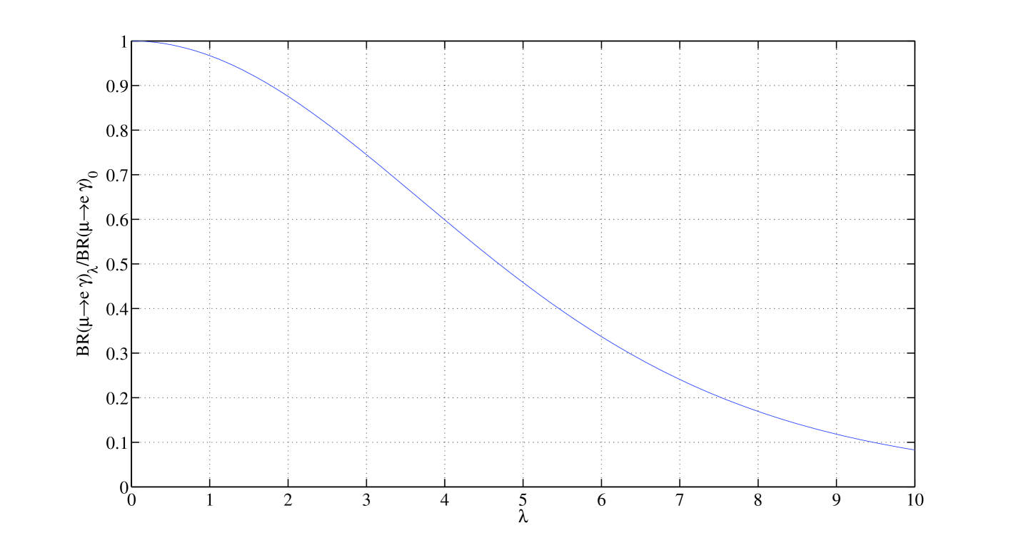
Figure 3: The branching ratio for $\mu\to e\gamma$ calculated incorporating the hidden sector in leading-logarithmic order as a function of $\lambda$, relative to the value without hidden-sector effects.

Using eq.(21), the branching ratio for $\mu\rightarrow e\gamma$ depends on $y_{21}$ as

$$\mathrm{BR}(\mu\rightarrow e\gamma)\sim\frac{\alpha^{3}}{G_{F}^{2}}\frac{|y_{21}|^{2}}{\tilde{m}_{S}^{8}}\tan^{2}\beta.$$ (23)

We see from Fig. 3 that the suppression of the branching ratio as a function of the fixed hidden-sector coupling becomes larger than a factor of two when $\lambda\gtrsim 5$. We should emphasize that in the above analysis we did not consider the shift in the scalar spectrum relative to the MSSM from hidden-sector dynamics, nor did we include the renormalization-group running of $\lambda$. Since the branching ratio depends inversely on sparticle masses to the eighth power (see eq.(23)), the changes in the sparticle spectra will have a non-negligible effect on the predicted rate. A competition will emerge between the suppression expected from the above analysis and the shifts in the sparticle spectra. We anticipate that in some regions where the hidden sector lowers the scalar spectrum sufficiently relative to the unaltered MSSM, the light scalars will dominate over the suppression factor, and yield an enhanced rate for ${\mu\to e\gamma}$. We explore these details in the next section.

Our analysis thus far assumed $\lambda$ was constant over the range of integration, in order to allow simple analytic treatment. In reality, the hidden-sector coupling $\lambda$ runs with its own $\beta$ function: $\beta_{\lambda}=(3/(32\pi^{2}))\lambda^{3}$. However, since the superpotential of eq.(3) by itself does not break supersymmetry, we must have additional hidden-sector interactions, so this model is just a toy, and not to be taken literally in detail. The point of the above discussion was simply to illustrate how a hidden sector self-interaction can influence the level of predicted charged LFV. In the following section, we examine the impact of the hidden sector in a model-independent fashion. Instead of hypothesizing a particular form of the coupling in the hidden sector, we parametrize the anomalous dimension itself. This parametrization allows us to examine both IR- and UV-free theories with ease.

4 LFV with general Hidden-Sector Effects

We saw from eq.(5) that in the cubic hidden superpotential theory we had

$$\frac{dk_{i}}{dt}=\frac{2\lambda^{*}\lambda}{16\pi^{2}}k_{i}+\mathrm{visible}\hskip 2.84526pt\mathrm{sector}\hskip 2.84526pt\mathrm{contributions}.$$ (24)

In order to examine general theories of the hidden sector, we require a parametrization that does not depend on the particulars of the hidden-sector implementation. For a general hidden sector we can define

$$\frac{dk_{i}}{dt}=\gamma(t)k_{i}+\mathrm{visible}\hskip 2.84526pt\mathrm{sector}\hskip 2.84526pt\mathrm{contributions},$$ (25)

where $\gamma(t)$ denotes the anomalous dimension contributed by the hidden sector. Instead of using $\gamma(t)$ from some specific theory as we did in the previous section, following our previous paper [49], we consider the parametrization [54],

$$\gamma(t)=\frac{1}{b_{\gamma}(s-a_{\gamma})},$$ (26)

where $b_{\gamma}$ and $a_{\gamma}$ are theory-dependent factors, and $s$ denotes the logarithm of the running scale. Depending on the location of the pole in $\gamma(t)$, we can examine both IR- and UV-free theories. We consider the following four cases for the anomalous dimension $\gamma(t)$: $b_{\gamma}=\pm 2/3$, $a_{\gamma}=\log(5\times 10^{11}\mathrm{GeV}/\mu),\log(5\times 10^{18}\mathrm{GeV}/\mu)$. We depict these cases in Fig. 4.

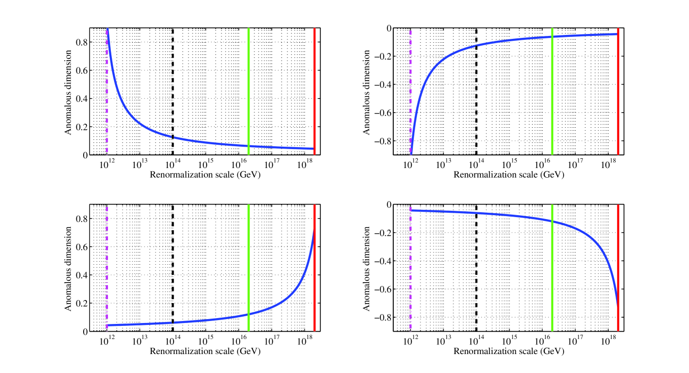
Figure 4: Four panels demonstrating the possible behaviours of the anomalous dimension outlined in the text. Top left: $b_{\gamma}=2/3$, $a_{\gamma}=\log(5\times 10^{11}\hskip 2.84526pt\mathrm{GeV}/\mu)$, top right: $b_{\gamma}=-2/3$, $a=\log(5\times 10^{11}\hskip 2.84526pt\mathrm{GeV}/\mu)$, bottom left: $b_{\gamma}=-2/3$, $a=\log(5\times 10^{18}\hskip 2.84526pt\mathrm{GeV}/\mu)$, bottom right: $b_{\gamma}=2/3$, $a=\log(5\times 10^{18}\hskip 2.84526pt\mathrm{GeV}/\mu)$. In each panel, the heavy solid line at $2\times 10^{18}$ GeV denotes the reduced Planck mass, the light solid line at $2\times 10^{16}$ GeV denotes the unification scale, the heavy dashed line at $10^{14}$ GeV represents the Majorana mass scale, and the light dashed-dotted line at $10^{12}$ GeV represents the hidden-sector mass scale.

By choosing the poles in either of two locations – just beyond the reduced Planck mass, or just below the hidden-sector scale ($10^{12}$ GeV) – we arrange that the hidden sector remains perturbative over the integration range and up to the reduced Planck mass itself. Once we reach the hidden-sector mass scale, we integrate out the hidden-sector physics, returning to the usual MSSM RGEs. As we see in Fig. 4, by placing the pole above the reduced Planck mass in the IR-free case, the magnitude of the anomalous dimension in the interval between the unification and the Majorana mass scales is smaller than in our UV-free case. We make this choice in order to ensure that the Landau pole in the IR-free case does not appear below the reduced Planck mass. In the following section, we will apply each of these cases to the MSSM with the Majorana scale set at $10^{14}$ GeV and with both hierarchical and degenerate Majorana gauge-singlet neutrinos, under the assumption of a normal hierarchy for the light neutrinos of the Standard Model. To determine the effect of the hidden sector on the predicted rate for ${\mu\to e\gamma}$, we run numerically the seesaw-extended MSSM RGEs including the hidden sector from the unification scale to the weak scale. We integrate out the Majorana gauge-singlet neutrinos at their associated scale and we also integrate out the hidden-sector effect at the hidden sector scale of $10^{12}$ GeV.

4.1 Hierarchical Gauge-Singlet Neutrinos

We recall from section 2 that the branching ratio $BR({\mu\to e\gamma})$ depends on the combination $\mathbf{Y}_{\nu}^{\dagger}\mathbf{Y}_{\nu}$, which through the Casas-Ibarra parametrization [52] can be expressed in terms of an orthogonal matrix $R$. In the case of hierarchical gauge-singlet Majorana neutrinos, one finds that (in the notation of section 2),

$$(\mathbf{Y}_{\nu})_{ij}\approx\sqrt{\mathcal{M}_{3}}\delta_{i3}R_{3l}(\sqrt{\kappa})_{l}U^{\dagger}_{lj}.$$ (27)

Thus, the branching ratio for ${\mu\to e\gamma}$ depends almost exclusively on one mixing angle in $R$, which we denote as $\theta_{1}$ (we are working under the assumption that $R$ is real). To demonstrate the effect of the hidden sector on the branching ratio, we choose a typical point in the MSSM parameter space: $\tan\beta=20$, $\mu>0$, $a_{0}=0$, $M_{0}=200$ GeV, $M_{1/2}=760$ GeV. In all cases, we set the hidden-sector mass scale at $10^{12}$ GeV.

We show in Fig. 5 the effect of the hidden sector on the branching ratio for ${\mu\to e\gamma}$ as a function of $\theta_{1}$. In each panel the solid blue curve denotes the prediction for the branching ratio in the absence of hidden-sector self-interactions, and the dashed red curve represents the prediction with the hidden-sector effect turned on. The top left panel displays the result for $b_{\gamma}=2/3$, $a_{\gamma}=\log(5\times 10^{11}\hskip 2.84526pt\mathrm{GeV}/\mu)$, the top right panel displays the result for $b_{\gamma}=-2/3$, $a=\log(5\times 10^{11}\hskip 2.84526pt\mathrm{GeV}/\mu)$, the bottom left panel displays the result for $b_{\gamma}=2/3$, $a=\log(5\times 10^{18}\hskip 2.84526pt\mathrm{GeV}/\mu)$, and the bottom left panel displays the result for $b_{\gamma}=-2/3$, $a=\log(5\times 10^{18}\hskip 2.84526pt\mathrm{GeV}/\mu)$.

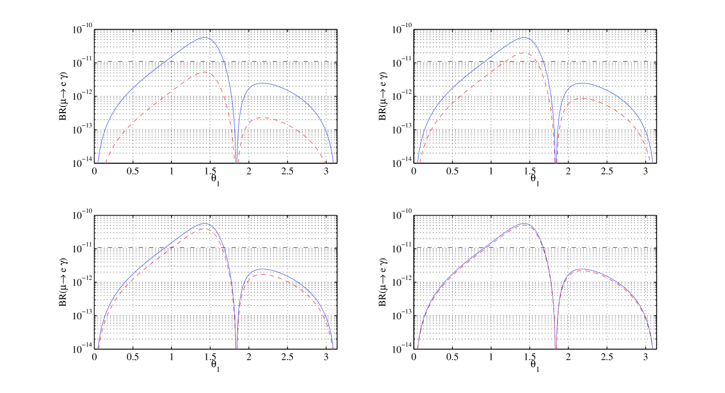
Figure 5: Four panels demonstrating the effect on ${\mu\to e\gamma}$ for the four behaviours of the anomalous dimension outlined in the text. Top left: $b_{\gamma}=2/3$, $a_{\gamma}=\log(5\times 10^{11}\hskip 2.84526pt\mathrm{GeV}/\mu)$, top right: $b_{\gamma}=-2/3$, $a=\log(5\times 10^{11}\hskip 2.84526pt\mathrm{GeV}/\mu)$, bottom left: $b_{\gamma}=2/3$, $a=\log(5\times 10^{18}\hskip 2.84526pt\mathrm{GeV}/\mu)$, and bottom right: $b_{\gamma}=-2/3$, $a=\log(5\times 10^{18}\hskip 2.84526pt\mathrm{GeV}/\mu)$.

We see that the largest suppression of the rate occurs for the UV-free anomalous dimension displayed in the top two panels. This observation simply reflects that in the UV-free setting we chose the pole of the anomalous dimension at $5\times 10^{11}$ GeV, a factor of two lower than the hidden sector scale, whilst in the IR-free case we placed the pole above the reduced Planck mass. As a result of these choices, the UV-free case has a larger anomalous dimension over the integration range. In this UV-free case, the anomalous dimension grows during the running of the RGEs from the unification scale to the hidden sector scale. Since the seesaw remains active until the Majorana scale is reached, we see that the growth in the hidden-sector anomalous dimension in the UV-free scenario serves to influence increasingly the rate for ${\mu\to e\gamma}$ – in this case suppressing the rate by up to an order of magnitude. This observation is consistent with our semi-analytic treatment in the previous section.

We can see how the allowed parameter space changes with the hidden-sector physics by examining the allowed parameter regions in the conventional CMSSM $M_{0}-M_{1/2}$ plane. In Fig. 6 we examine the hierarchical Majorana gauge-singlet neutrino case with $\theta_{1}=1.4$, displaying the large effect that the hidden sector may have on the predicted rate for ${\mu\to e\gamma}$. The solid white area in each of the three panels indicates the region that is currently excluded by the experimental upper limit ($\mathrm{BR}({\mu\to e\gamma})<1.2\times 10^{-11}$). The left panel displays the allowed region with the hidden sector effect turned off; the second panel shows the effect with the allowed regions for $b_{\gamma}=2/3$, $a_{\gamma}=\log(5\times 10^{11}\hskip 2.84526pt\mathrm{GeV}/\mu)$, and the third panel displays the effect with $b_{\gamma}=-2/3$, $a_{\gamma}=\log(5\times 10^{11}\hskip 2.84526pt\mathrm{GeV}/\mu)$. In each case we set the Majorana mass scale to $10^{14}$ GeV and the hidden-sector scale to $10^{12}$ GeV.

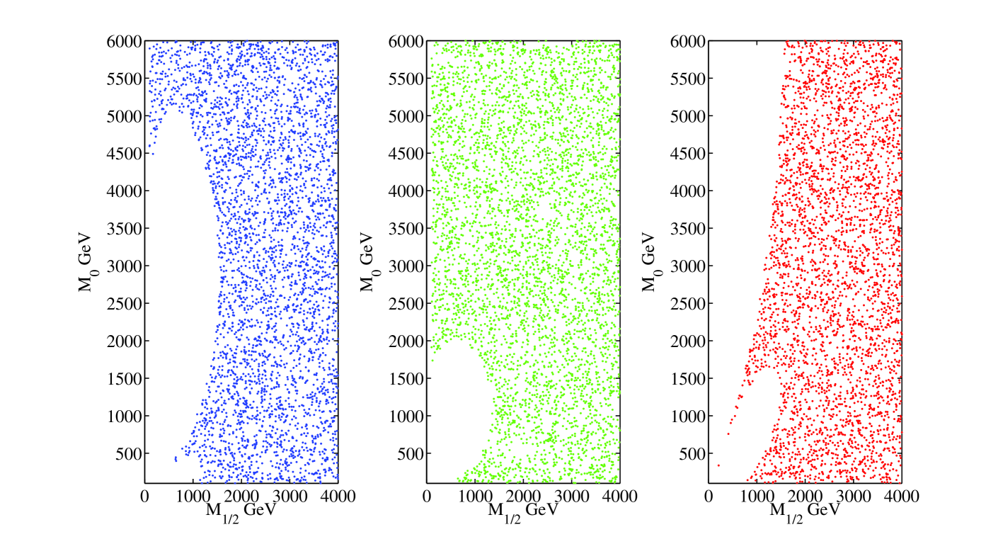
Figure 6: The allowed parameter space with $BR({\mu\to e\gamma})<1.2\times 10^{-11}$ in the presence of hierarchical gauge-singlet neutrinos and a UV-free hidden-sector theory, with the solid white regions denoting excluded regions. Left panel: allowed parameter space without hidden-sector dynamics, middle panel: allowed parameter region with $b_{\gamma}=2/3$, $a_{\gamma}=\log(5\times 10^{11}\hskip 2.84526pt\mathrm{GeV}/\mu)$, and right panel: allowed parameter region with $b_{\gamma}=-2/3$, $a_{\gamma}=\log(5\times 10^{11}\hskip 2.84526pt\mathrm{GeV}/\mu)$. In all cases $M_{R}=10^{14}$ GeV, $\mu>0$, $\tan\beta=20$, $a_{0}=0$.

We see that the hidden sector can change the allowed parameter space quite dramatically. Comparing the last two panels with the first one, we see that some regions that were excluded have become allowed and regions that were allowed have become excluded. These figures indicate the subtle effects the hidden sector may have. From the semi-analytic treatment in the previous section, we saw that for a large enough hidden-sector coupling, we expect the rate for ${\mu\to e\gamma}$ to become suppressed. However, as mentioned earlier, the hidden sector also alters the sparticle spectrum, specifically the mass eigenvalues of the scalar particles, and this has a nontrivial effect on the branching ratio for ${\mu\to e\gamma}$. In order to determine the full effect of the hidden sector on the branching ratio for ${\mu\to e\gamma}$, we require a full numerical treatment as displayed in Fig. 6. In regions where the hidden sector serves to eliminate parameter space, the change in the sparticle spectrum is the dominant effect.

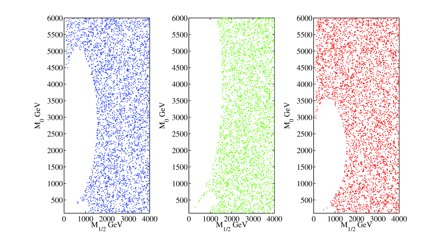
Figure 7: Hierarchical gauge-singlet neutrinos with an IR-free hidden-sector theory, displaying the allowed parameter space with $BR({\mu\to e\gamma})<1.2\times 10^{-11}$, with the solid white regions denoting excluded regions. Left panel: allowed parameter space without hidden sector dynamics, middle panel: allowed parameter region with $b_{\gamma}=2/3$, $a_{\gamma}=\log(5\times 10^{18}\hskip 2.84526pt\mathrm{GeV}/\mu)$, and right panel: allowed parameter region with $b_{\gamma}=-2/3$, $a_{\gamma}=\log(5\times 10^{18}\hskip 2.84526pt\mathrm{GeV}/\mu)$. In all cases $M_{R}=10^{14}$ GeV, $M_{\mathrm{hidden}}\sim 10^{12}$, $\mu>0$, $\tan\beta=20$, and $a_{0}=0$.

In Fig. 7, we show the effect of the hidden sector with an IR-free anomalous dimension in the same parameter space as Fig. 6. Again, we see that the hidden sector can change dramatically the allowed parameter space. The first panel displays the allowed region with the hidden-sector effect turned off, the second panel shows the effect on the allowed regions for $b_{\gamma}=2/3$, $a_{\gamma}=\log(5\times 10^{18}\hskip 2.84526pt\mathrm{GeV}/\mu)$, and the third panel displays the effect with $b_{\gamma}=-2/3$, $a_{\gamma}=\log(5\times 10^{18}\hskip 2.84526pt\mathrm{GeV}/\mu)$. In all cases we have taken $\theta_{1}=1.4$ with the Majorana mass scale at $10^{14}$ GeV and the hidden sector mass scale at $10^{12}$ GeV.

4.2 Degenerate Gauge-Singlet Neutrinos

In the degenerate gauge-singlet neutrino case the combination $\mathbf{Y}_{\nu}\mathbf{Y}_{\nu}^{\dagger}$ yields no dependence on any particular angle in the orthogonal matrix $R$. In this case, once $\mathbf{Y}_{\nu}\mathbf{Y}_{\nu}^{\dagger}$ is given, the branching ratio is fully determined. We begin by displaying the parameter space in the $M_{0}-M_{1/2}$ plane. The three panels in Fig. 8 show the changes in the allowed parmeter space in the presence of the hidden sector. The first panel displays the allowed region with the hidden sector effect turned off, the second panel shows the effect with the allowed regions for $b_{\gamma}=2/3$, $a_{\gamma}=\log(5\times 10^{11}\hskip 2.84526pt\mathrm{GeV}/\mu)$, and the third panel displays the effect with $b_{\gamma}=-2/3$, $a_{\gamma}=\log(5\times 10^{11}\hskip 2.84526pt\mathrm{GeV}/\mu)$. In all cases we have taken $\theta_{1}=1.4$ with the Majorana scale at $10^{14}$ GeV and the hidden-sector scale at $10^{12}$ GeV.

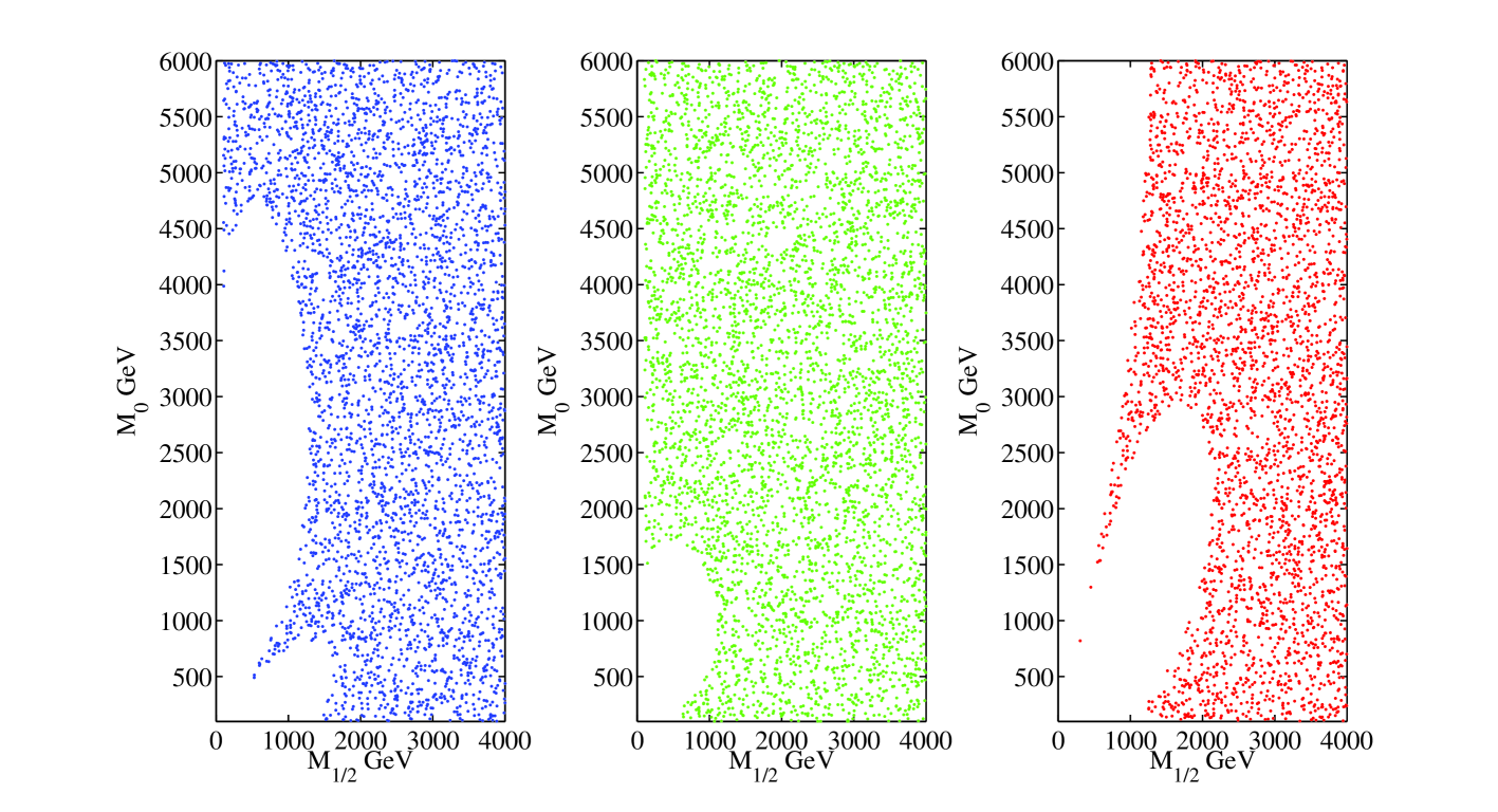
Figure 8: The case of degenerate gauge-singlet neutrinos with an UV-free hidden-sector theory, displaying the allowed parameter space with $BR({\mu\to e\gamma})<1.2\times 10^{-11}$, with the solid white regions denoting excluded regions. Left panel: allowed parameter space without hidden-sector dynamics, middle panel: allowed parameter region with $b_{\gamma}=2/3$, $a_{\gamma}=\log(5\times 10^{11}\hskip 2.84526pt\mathrm{GeV}/\mu)$, and right panel: allowed parameter region with $b_{\gamma}=-2/3$, $a_{\gamma}=\log(5\times 10^{11}\hskip 2.84526pt\mathrm{GeV}/\mu)$. In all cases $M_{R}=10^{14}$ GeV, $M_{\mathrm{hidden}}=10^{12}$ GeV, $\mu>0$, $\tan\beta=20$, and $a_{0}=0$.

In Fig. 9 we repeat the analysis for the IR-free anomalous dimension case with parameters $b_{\gamma}=2/3$, $a_{\gamma}=\log(5\times 10^{18}\hskip 2.84526pt\mathrm{GeV}/\mu)$. The third panel displays the effect with $b_{\gamma}=-2/3$, $a_{\gamma}=\log(5\times 10^{18}\hskip 2.84526pt\mathrm{GeV}/\mu)$, respectively. Again we see the competition between the expected suppression in the rate for ${\mu\to e\gamma}$ and the alteration of the sparticle spectrum. In either case we can see that the hidden sector has a dramatic effect on the rate for ${\mu\to e\gamma}$ and that a knowledge of the hidden sector is not only required to make accurate predictions of the low-energy mass spectrum, but is also required to predict the level of expected charged-lepton flavour violation.

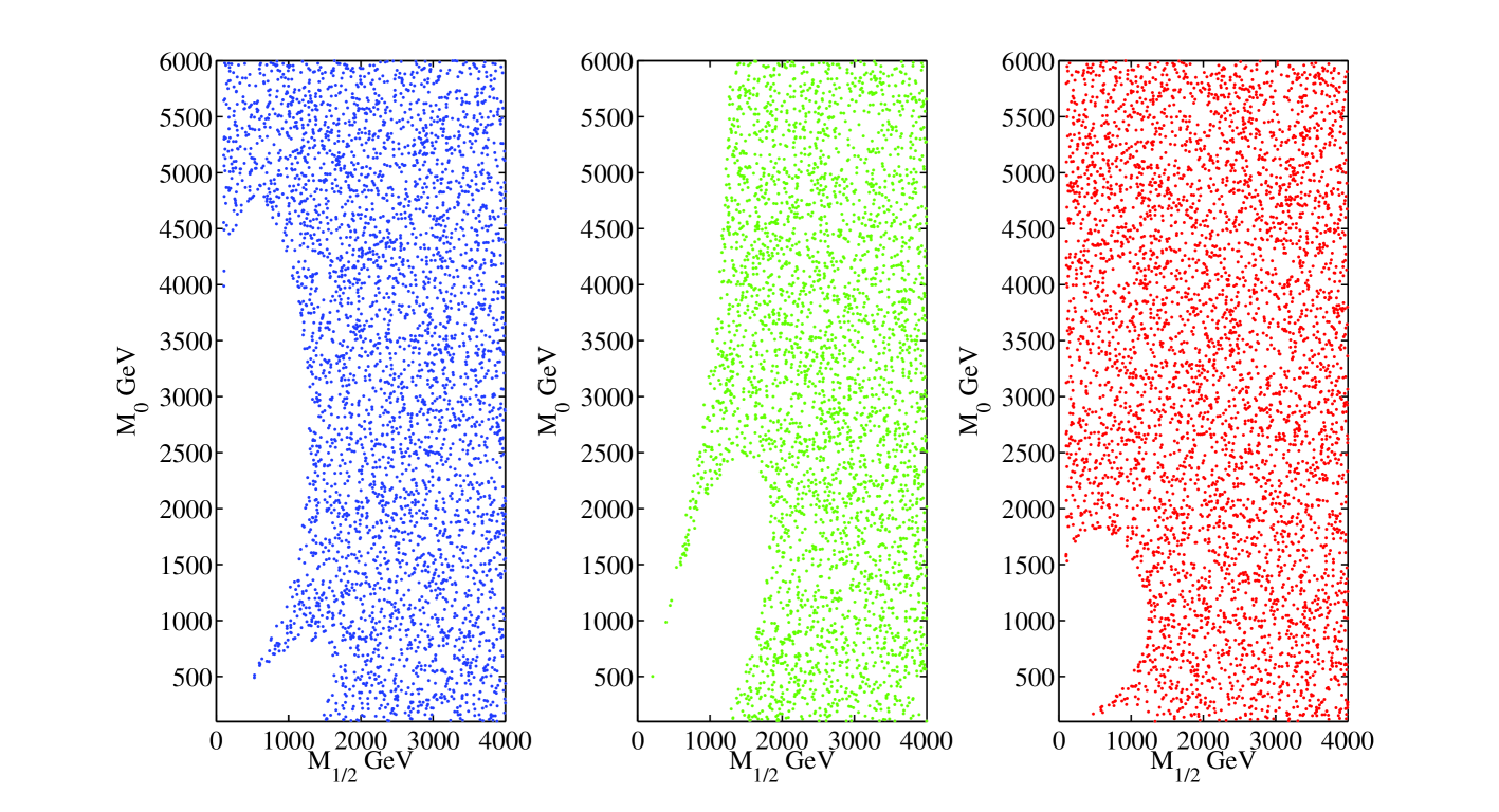
Figure 9: Degenerate gauge-singlet neutrinos with an IR-free hidden-sector theory, displaying the allowed parameter space with $BR({\mu\to e\gamma})<1.2\times 10^{-11}$, with the solid white regions denoting excluded regions. Left panel: allowed parameter space without hidden-sector dynamics, middle panel: allowed parameter region with $b_{\gamma}=2/3$, $a_{\gamma}=\log(5\times 10^{18}\hskip 2.84526pt\mathrm{GeV}/\mu)$, and right panel: allowed parameter region with $b_{\gamma}=-2/3$, $a_{\gamma}=\log(5\times 10^{18}\hskip 2.84526pt\mathrm{GeV}/\mu)$. In all cases $M_{R}=10^{14}$ GeV, $M_{\mathrm{hidden}}=10^{12}$ GeV, $\mu>0$, $\tan\beta=20$, and $a_{0}=0$.

5 Hidden-Sector Dynamics and Seesaw Reconstruction

Since the hidden sector affects not only the supersymmetric spectrum but also the radiatively-induced seesaw charged LFV, the hidden sector impacts the ability to reconstruct the seesaw from low-energy observations. As we see from eq.(21), charged LFV fixes the elements of $\mathbf{Y}_{\nu}\mathbf{Y}_{\nu}^{\dagger}$, while low-energy neutrino observations determine the PMNS matrix and $\kappa$ in the Casas-Ibarra parametrization [52], eq.(1). It has been shown [55] that, in principle, in the seesaw extension of the MSSM, a unique map $\mathbf{Y}_{\nu}\mathbf{Y}_{\nu}^{\dagger},\kappa\rightarrow\mathbf{Y}_{\nu},\mathcal{M}$ exists, and thus the seesaw parameters can be reconstructed from low-energy data. What is important in this reconstruction is that in the seesaw extension of the MSSM all the non-seesaw interactions are in principle known from low-energy data, so the RGE mixing responsible for the $\mathbf{Y}_{\nu}\mathbf{Y}_{\nu}^{\dagger}$ generating charged LFV has only the seesaw parameters as unknowns.

In our preceding paper [49], we made the case that, for hidden sectors that could be effectively parametrized by a two-parameter characterization of the anomalous dimension of the dominant scalar mass-squared mediation operator (after removing external line wave-function renormalization effects by rescaling the input parameters at $M$) that the parameters could in principle be fit, and in most cases distinguished from other parametrizations by measurements of the low-energy soft supersymmetry-breaking terms. This reconstruction can be done using combinations of the soft parameters which are unaffected by the seesaw.

In these circumstances one would still be able to do seesaw reconstruction, as all the non-seesaw contributions to the soft-parameter RGEs would be known. However, the reconstruction does depend on the assumption that the slepton soft mass matrices at the mediation scale $M$ are proportional to the identity, as in the CMSSM case.

Hence, if the LHC and a linear collider reveal evidence for a distorted superpartner spectrum, consistent with strong hidden-sector dynamics, it will be essential to reconstruct this dynamics as proposed in [49] first, before one can use other low-energy observables, such as charged-lepton flavour violation, to reconstruct the parameters of the seesaw mechanism.

Conversely, if the hidden sector dynamics is sufficiently complicated to defy convenient parametrization and experimental determination, then the unknown hidden-sector contributions to the RGE flow of the soft supersymmetry-breaking parameters will present an irreducible obstacle to using low-energy data to determine seesaw parameters.

6 Comments and Conclusions

Recent theoretical observations have demonstrated that low-energy predictions in supersymmetric models, such as the supersymmetric spectrum itself, can be significantly influenced by a dynamical hidden sector used to break supersymmetry [45, 46, 47, 48]. In this paper, we have examined the effect of a dynamical hidden sector on seesaw induced charged-lepton flavour violation. Since both the seesaw sector and the hidden sector sit at intermediate scales, an interval exists where both effects are active during the renormalization group running from the unification scale to the weak scale. The combined effect may alter the usually expected charged-lepton flavour violation in the seesaw extension of the MSSM.

In our analysis, we parameterized the effect of the hidden sector through a simple anomalous-dimension Ansatz. In any realistic model, the actual behaviour of the hidden-sector coupling would be determined by the theory, but we see that from our simple parametrization that we can capture the effect of moderately-coupled IR-free and UV-free theories. At a comparison point, we see that the self-coupling in the cubic superpotential theory requires $\lambda\gtrsim 5$ in order for the hidden sector to have a significant effect on the rate for ${\mu\to e\gamma}$. Our model-independent parametrizations ensured perturbativity in the range of integration and, in particular, we ensured the the hidden sector remains perturbative up to the reduced Planck scale. In order to generate a large effect on ${\mu\to e\gamma}$, we need a moderately strongly-coupled hidden sector. In the UV-free theory, we placed the pole of the anomalous dimension just below the hidden-sector scale itself. This ensured that the anomalous dimension becomes large over the range where the seesaw is active. If the hidden sector does not become strongly coupled until well outside the interval between the hidden-sector and Majorana scales, the effect on flavour violation becomes minimal. We can see this effect with the IR-free theory where we place the pole just above the reduced Planck mass. Since we started running the theory at $M_{X}=2\times 10^{16}$ GeV, the anomalous dimension started from a smaller value relative to the end-point of the UV-free anomalous dimension in our examples.

Finally, we noted that, in the presence of strongly-coupled hidden sectors whose dynamics distorts significantly the pattern of soft supersymmetry-breaking scalar masses-squared, the ability to use soft parameters in a reconstruction of the seesaw depends on establishing previously the ability to use the TeV-scale observables to reconstruct the hidden-sector dynamics in ways that we have previously analyzed in [49]. Otherwise, the observable effects of the hidden sector may impede our view of the seesaw sector.

Appendix: One-Loop MSSM Calculation for $l_{j}\rightarrow l_{i}+\gamma$

We calculate the rate for ${\mu\to e\gamma}$ at one loop in the MSSM after running the full system of MSSM RGEs. We follow the notation in [56]; similar formulae can be found in [51]. The interactions leading to the LFV process $l_{j}\rightarrow l_{i}+\gamma$ involve the effective Lagrangians describing the neutralino-lepton-slepton and the chargino-lepton-sneutrino systems. Written in the mass eigenbasis where $\mathbf{O}_{\mathrm{ne}}$ diagonalizes the neutralino mass matrix, $\mathbf{O}_{\mathrm{L}}$ and $\mathbf{O}_{\mathrm{R}}$ diagonalize the chargino mass matrix, $\mathbf{U}_{\mathrm{\tilde{f}}}$ diagonalizes the charged-slepton mass matrix, and $\mathbf{U}_{\mathrm{\tilde{n}}}$ diagonalizes the weak-scale sneutrino mass matrix, we have

$$\mathcal{L}=\sum_{i=1}^{3}\sum_{a=1}^{4}\sum_{b=1}^{6}N^{\mathrm{L}}_{iab}\tilde{f}_{b}E_{i}\tilde{\chi}^{0}_{a}+N^{\mathrm{R}*}_{iab}\tilde{f}^{*}_{b}e_{i}\tilde{\chi}^{0}_{a}\;+\;\mathrm{c.\;c.}$$ (28)

and

$$\mathcal{L}=\sum_{i=1}^{3}\sum_{a=1}^{2}\sum_{b=1}^{3}C^{\mathrm{L}}_{iab}\tilde{\nu}_{b}E_{i}\tilde{\chi}^{-}_{a}+C^{\mathrm{R}*}_{iab}\tilde{\nu}^{*}_{b}e_{i}\tilde{\chi}^{+}_{a},\;+\;\mathrm{c.\;c.}$$ (29)

where

$$N^{\mathrm{L}}_{iab} = -\frac{g_{2}}{\sqrt{2}}\left(2\tan\theta_{\mathrm{W}}\left(\mathbf{U}_{\mathrm{\tilde{f}}}\right)^{*}_{b\left(i+3\right)}\left(\mathbf{O}_{\mathrm{ne}}\right)_{a1}+\frac{m_{\mathrm{l}_{i}}}{m_{\mathrm{W}}\cos\beta}\left(\mathbf{U}_{\mathrm{\tilde{f}}}\right)^{*}_{bi}\left(\mathbf{O}_{\mathrm{ne}}\right)_{a3}\right),$$ (30)

$$N^{\mathrm{R}}_{iab} = \frac{g_{2}}{\sqrt{2}}\left(\tan\theta_{\mathrm{W}}\left(\mathbf{U}_{\mathrm{\tilde{f}}}\right)^{*}_{bi}\left(\mathbf{O}_{\mathrm{ne}}\right)_{a1}+\left(\mathbf{U}_{\mathrm{\tilde{f}}}\right)^{*}_{bi}\left(\mathbf{O}_{\mathrm{ne}}\right)_{a2}-\frac{m_{\mathrm{l}_{i}}}{m_{\mathrm{W}}\cos\beta}\left(\mathbf{U}_{\mathrm{\tilde{f}}}\right)^{*}_{b\left(i+3\right)}\left(\mathbf{O}_{\mathrm{ne}}\right)_{a3}\right),\quad\quad$$ (31)

, and

$$C^{\mathrm{L}}_{iab} = \frac{g_{2}m_{\mathrm{l}_{i}}}{\sqrt{2}m_{\mathrm{W}}\cos\beta}\left(\mathbf{O}_{\mathrm{L}}\right)_{a2}\left(\mathbf{U}_{\mathrm{\tilde{n}}}\right)^{*}_{bi},$$ (32)

$$C^{\mathrm{R}}_{iab} = -g_{2}\left(\mathbf{O}_{\mathrm{R}}\right)_{a1}\left(\mathbf{U}_{\mathrm{\tilde{n}}}\right)^{*}_{bi}.$$ (33)

The on-shell amplitude for $l_{j}\rightarrow l_{i}+\gamma$ has the general form

$$\mathcal{M}=e\epsilon^{*}_{\mu}\bar{l}_{i}\left(p-q\right)\left(im_{\mathrm{l}_{j}}\sigma^{\mu\nu}q_{\nu}\left(A_{\mathrm{L}}\mathrm{L}+A_{\mathrm{R}}\mathrm{R}\right)\right)l_{j}\left(p\right),$$ (34)

where we have used Dirac spinors $l_{i}\left(p-q\right)$ and $l_{j}\left(p\right)$ for the charged leptons $i$ and $j$ with momenta $p-q$ and $p$, respectively; $\mathrm{L}=\left(1-\gamma^{5}\right)/2$ and $\mathrm{R}=\left(1+\gamma^{5}\right)/2$. Each of the dipole coefficients $A_{\mathrm{L}}$ and $A_{\mathrm{R}}$ receives contributions from the neutralino-lepton-slepton and chargino-lepton-sneutrino interactions, namely,

$$A_{\mathrm{L}}=A_{\mathrm{L}}^{\mathrm{(n)}}+A_{\mathrm{L}}^{\mathrm{(c)}},$$ (35)

and

$$A_{\mathrm{R}}=A_{\mathrm{R}}^{\mathrm{(n)}}+A_{\mathrm{R}}^{\mathrm{(c)}},$$ (36)

where $A_{\mathrm{L}}^{\mathrm{(n)}}$, $A_{\mathrm{R}}^{\mathrm{(n)}}$, $A_{\mathrm{L}}^{\mathrm{(c)}}$, $A_{\mathrm{R}}^{\mathrm{(c)}}$ can be evaluated from the Feynman diagrams in Fig. 2;

$$A_{\mathrm{L}}^{\mathrm{(n)}} = \phantom{-}\frac{1}{32\pi^{2}}\sum_{a=1}^{4}\sum_{b=1}^{6}\frac{1}{m^{2}_{\mathrm{\tilde{f}}_{b}}}\left(N^{\mathrm{L}}_{iab}N^{\mathrm{L}*}_{jab}J_{1}\left(\frac{M^{2}_{\tilde{\chi}^{0}_{a}}}{m^{2}_{\tilde{l}_{b}}}\right)\right.$$ (37)

$$\left.+N^{\mathrm{L}}_{iab}N^{\mathrm{R}*}_{jab}\frac{\left|M_{\tilde{\chi}^{0}_{a}}\right|}{m_{l_{j}}}J_{2}\left(\frac{M^{2}_{\tilde{\chi}^{0}_{a}}}{m^{2}_{\tilde{l}_{b}}}\right)\right),$$

$$A_{\mathrm{L}}^{\mathrm{(c)}} = -\frac{1}{32\pi^{2}}\sum_{a=1}^{2}\sum_{b=1}^{3}\frac{1}{m^{2}_{\tilde{\nu}_{b}}}\left(C^{\mathrm{L}}_{iab}C^{\mathrm{L}*}_{jab}J_{3}\left(\frac{M^{2}_{\tilde{\chi}^{-}_{a}}}{m^{2}_{\tilde{\nu}_{b}}}\right)\right.$$ (38)

$$+\left.C^{\mathrm{L}}_{iab}C^{\mathrm{R}*}_{jab}\frac{M_{\tilde{\chi}^{-}_{a}}}{m_{l_{j}}}J_{4}\left(\frac{M^{2}_{\tilde{\chi}^{-}_{a}}}{m^{2}_{\tilde{\nu}_{b}}}\right)\right),$$

$$A_{\mathrm{R}}^{\mathrm{(n)}} = \left.A_{\mathrm{L}}^{\mathrm{(n)}}\right|_{L\leftrightarrow R},$$ (39)

$$A_{\mathrm{R}}^{\mathrm{(c)}} = \left.A_{\mathrm{L}}^{\mathrm{(c)}}\right|_{L\leftrightarrow R}.$$ (40)

The functions $J_{1}\left(x\right)$, $J_{2}\left(x\right)$, $J_{3}\left(x\right)$, $J_{4}\left(x\right)$ are defined as

$$J_{1}\left(x\right) = \frac{1-6x+3x^{2}+2x^{3}-6x^{2}\ln x}{6\left(1-x\right)^{4}},$$ (41)

$$J_{2}\left(x\right) = \frac{1-x^{2}+2x\ln x}{\left(1-x\right)^{3}},$$ (42)

$$J_{3}\left(x\right) = \frac{2+3x-6x^{2}+x^{3}+6x\ln x}{6\left(1-x\right)^{4}},$$ (43)

$$J_{4}\left(x\right) = \frac{-3+4x-x^{2}+2\ln x}{\left(1-x\right)^{3}}.$$ (44)

Finally, the decay rate for $l^{-}_{j}\rightarrow l^{-}_{i}+\gamma$ is given by

$$\Gamma\left(l^{-}_{j}\rightarrow l^{-}_{i}+\gamma\right)=\frac{e^{2}}{16\pi}m_{l_{j}}^{5}\left(\left|A_{\mathrm{L}}\right|^{2}+\left|A_{\mathrm{R}}\right|^{2}\right),$$ (45)

and $i=1$, $j=2$ for $\mu\rightarrow e+\gamma$.

References

- [1] H. P. Nilles, Phys. Rept. 110, 1 (1984).
- [2] H. E. Haber and G. L. Kane, Phys. Rept. 117, 75 (1985).
- [3] J. R. Ellis, S. Heinemeyer, K. A. Olive, A. M. Weber, and G. Weiglein, JHEP 08, 083 (2007), arXiv:0706.0652 [hep-ph].
- [4] M. Drees, R. Godbole, and P. Roy, Hackensack, USA: World Scientific (2004) 555 p.
- [5] P. Ramond, Reading, Mass., Perseus Books, 1999.
- [6] J. Terning, Oxford, UK: Clarendon (2006) 324 p.
- [7] S. Weinberg, Cambridge, UK: Univ. Pr. (2000) 419 p.
- [8] S. Dimopoulos and H. Georgi, Nucl. Phys. B193, 150 (1981).
- [9] H. Georgi, H. R. Quinn, and S. Weinberg, Phys. Rev. Lett. 33, 451 (1974).
- [10] S. Dimopoulos, S. Raby, and F. Wilczek, Phys. Rev. D24, 1681 (1981).
- [11] B. T. Cleveland et al., Astrophys. J. 496, 505 (1998).
- [12] SNO, Q. R. Ahmad et al., Phys. Rev. Lett. 87, 071301 (2001), nucl-ex/0106015.
- [13] SNO, Q. R. Ahmad et al., Phys. Rev. Lett. 89, 011301 (2002), nucl-ex/0204008.
- [14] SNO, Q. R. Ahmad et al., Phys. Rev. Lett. 89, 011302 (2002), nucl-ex/0204009.
- [15] Super-Kamiokande, Y. Fukuda et al., Phys. Rev. Lett. 81, 1562 (1998), hep-ex/9807003.
- [16] Super-Kamiokande, Y. Fukuda et al., Phys. Rev. Lett. 82, 2644 (1999), hep-ex/9812014.
- [17] Super-Kamiokande, S. Fukuda et al., Phys. Rev. Lett. 85, 3999 (2000), hep-ex/0009001.
- [18] Super-Kamiokande, S. Fukuda et al., Phys. Rev. Lett. 86, 5656 (2001), hep-ex/0103033.
- [19] KamLAND, K. Eguchi et al., Phys. Rev. Lett. 90, 021802 (2003), hep-ex/0212021.
- [20] KamLAND, T. Araki et al., Phys. Rev. Lett. 94, 081801 (2005), hep-ex/0406035.
- [21] K2K, M. H. Ahn et al., Phys. Rev. Lett. 90, 041801 (2003), hep-ex/0212007.
- [22] K2K, E. Aliu et al., Phys. Rev. Lett. 94, 081802 (2005), hep-ex/0411038.
- [23] GALLEX, W. Hampel et al., Phys. Lett. B447, 127 (1999).
- [24] GALLEX, P. Anselmann et al., Phys. Lett. B357, 237 (1995).
- [25] SAGE, J. N. Abdurashitov et al., J. Exp. Theor. Phys. 95, 181 (2002), astro-ph/0204245.
- [26] SAGE, J. N. Abdurashitov et al., Phys. Rev. Lett. 83, 4686 (1999), astro-ph/9907131.
- [27] SAGE, J. N. Abdurashitov et al., Phys. Lett. B328, 234 (1994).
- [28] M. Fukugita and T. Yanagida, Physics of neutrinos and applications to astrophysics , Berlin, Germany: Springer (2003) 593 p.
- [29] B. A. Campbell and D. W. Maybury, JHEP 04, 077 (2007), hep-ph/0603053.
- [30] J. A. Casas, J. R. Espinosa, A. Ibarra, and I. Navarro, Nucl. Phys. B569, 82 (2000), hep-ph/9905381.
- [31] S. Antusch, M. Drees, J. Kersten, M. Lindner, and M. Ratz, Phys. Lett. B519, 238 (2001), hep-ph/0108005.
- [32] S. Antusch, J. Kersten, M. Lindner, and M. Ratz, Nucl. Phys. B674, 401 (2003), hep-ph/0305273.
- [33] P. Van Nieuwenhuizen, Phys. Rept. 68, 189 (1981).
- [34] M. Dine, W. Fischler, and M. Srednicki, Nucl. Phys. B189, 575 (1981).
- [35] S. Dimopoulos and S. Raby, Nucl. Phys. B192, 353 (1981).
- [36] C. R. Nappi and B. A. Ovrut, Phys. Lett. B113, 175 (1982).
- [37] R. Barbieri, S. Ferrara, and C. A. Savoy, Phys. Lett. B119, 343 (1982).
- [38] L. Alvarez-Gaume, M. Claudson, and M. B. Wise, Nucl. Phys. B207, 96 (1982).
- [39] S. Dimopoulos and S. Raby, Nucl. Phys. B219, 479 (1983).
- [40] M. Dine and A. E. Nelson, Phys. Rev. D48, 1277 (1993), hep-ph/9303230.
- [41] M. Dine, A. E. Nelson, and Y. Shirman, Phys. Rev. D51, 1362 (1995), hep-ph/9408384.
- [42] M. Dine, A. E. Nelson, Y. Nir, and Y. Shirman, Phys. Rev. D53, 2658 (1996), hep-ph/9507378.
- [43] G. F. Giudice and R. Rattazzi, Phys. Rept. 322, 419 (1999), hep-ph/9801271.
- [44] K. Choi and H. P. Nilles, JHEP 04, 006 (2007), hep-ph/0702146.
- [45] M. Dine et al., Phys. Rev. D70, 045023 (2004), hep-ph/0405159.
- [46] A. G. Cohen, T. S. Roy, and M. Schmaltz, JHEP 02, 027 (2007), hep-ph/0612100.
- [47] H. Murayama, Y. Nomura, and D. Poland, Phys. Rev. D77, 015005 (2008), arXiv:0709.0775 [hep-ph].
- [48] M. Schmaltz and R. Sundrum, JHEP 11, 011 (2006), hep-th/0608051.
- [49] Bruce A. Campbell, John Ellis and D. W. Maybury, arXiv.0810.4877 [hep-ph].
- [50] F. Borzumati and A. Masiero, Phys. Rev. Lett. 57, 961 (1986).
- [51] J. Hisano, T. Moroi, K. Tobe, and M. Yamaguchi, Phys. Rev. D53, 2442 (1996), hep-ph/9510309.
- [52] J. A. Casas and A. Ibarra, Nucl. Phys. B618, 171 (2001), hep-ph/0103065.
- [53] T. Mori, Nucl. Phys. Proc. Suppl. 111, 194 (2002).
- [54] Graham Ross, unpublished.
- [55] S. Davidson and A. Ibarra, JHEP 09, 013 (2001), hep-ph/0104076.
- [56] E. Jankowski and D. W. Maybury, Phys. Rev. D70, 035004 (2004), hep-ph/0401132.