Multiwavelength Signatures of Magnetic Activity from Young Stellar Objects in the LkH$\alpha$101 Cluster

Abstract

We describe the results of our multi-wavelength observing campaign on the young stellar objects in the LkH$\alpha$101 cluster. Our simultaneous X-ray and multi-frequency radio observations are unique in providing simultaneous constraints on short-timescale variability at both wavelengths as well as constraints on the thermal or nonthermal nature of radio emission from young stars. Focussing in on radio-emitting objects and the multi-wavelength data obtained for them, we find that multi-frequency radio data indicate nonthermal emission even in objects with infrared evidence for disks. We find radio variability on timescales of decades, days and hours. About half of the objects with X-ray and radio detections were variable at X-ray wavelengths, despite lacking large-scale flares or large variations. Variability appears to be a bigger factor affecting radio emission than X-ray emission. A star with infrared evidence for a disk, [BW88] 3, was observed in the decay phase of radio flare. In this object and another ([BW88] 1), we find an inverse correlation between radio flux and spectral index which contrasts with behavior seen in the Sun and active stars. We interpret this behavior as the repopulation of the hardest energy electrons due to particle acceleration. A radio and X-ray source lacking an infrared counterpart, [BW88] 1, may be near the substellar limit; its radio properties are similar to other cluster members, but its much higher radio to X-ray luminosity ratio is reminiscent of behavior in nearby very low mass stars/brown dwarfs. We find no correspondence between signatures of particle acceleration and those of plasma heating, both time-averaged and time-variable. The lack of correlated temporal variability in multi-wavelength behavior, the breakdown of multi-wavelength correlations of time-averaged luminosities, and the optical thickness of X-ray-emitting material at radio wavelengths support the idea that radio and X-ray emission on young stars are physically and/or energetically distinct.

1 Introduction

Magnetic fields play an important, but poorly understood, role in the formation and further evolution of late-type stars. The influence of magnetic fields in stellar environments can be seen, for example, in X-ray emission from gas which has been magnetically heated to coronal temperatures, and radio emission arising from the action of nonthermal particles in the presence of magnetic fields. In the last 20 years, remarkable advances in the detection and study of stellar sources at X-ray and radio wavelengths have revealed an intimate connection between radio and X-ray luminosities of late-type stars. This relationship extends from time-averaged estimates of the presumably steady emission, to spectacular examples of flare enhancements when studied simultaneously with multiple wavelengths. Yet the underlying connection is still not well constrained. Most of the observational multi-wavelength studies of magnetically-induced flare activity on late-type stars have concentrated on targeted studies of nearby, extremely active stars. The goal of the current project is to investigate a region of active star formation, using simultaneous X-ray and radio observations, to constrain the relationship of these emissions in both steady and varying emission. This will allow us to determine the extent to which the solar paradigm can be carried in these very active young stars.

1.1 The Stellar X-ray–Radio Connection

At first glance, there is an obvious disconnect between X-ray and radio emission from active stars: X-ray observations are well described by optically thin, thermal, high temperature plasma generally seen in a distribution between a few MK and tens of MK (few keV), while radio observations generally probe nonthermal populations of accelerated electrons with energies of a few MeV. Yet among several classes of active stars and solar flares, a tight relation between X-ray and radio luminosities is found, L${}_{X}/$L_R $\sim 10^{15.5\pm 0.5}$ Hz (Güdel & Benz, 1993; Benz & Güdel, 1994). This relation extends from solar microflares up to the most energetic coronal sources (in radio and X-rays): the weak T Tauri stars (wTTs; Class III objects). The observational relationship invites an interpretation based on a common origin – particle acceleration and thermal coronal heating, separate but related steps in the flow of energy after a magnetic reconnection event, as inferred from solar and stellar flare studies.

On the Sun, the observed relationship between nonthermal processes and thermal coronal emission during individual transient impulsive flare events is well known (Neupert, 1968) and has given rise to a standard flare scenario. Particles are accelerated high in the corona in connection with a reconnection event, and downwardly-directed electron beams “inject” these energetic particles into coronal loops, which act as a magnetic trap. Radio gyrosynchrotron emission occurs from trapped particles; those which precipitate due to pitch-angle scattering encounter the dense chromosphere where they are collisionally stopped, depositing their energy in the ambient plasma. The temperate chromospheric material becomes heated to coronal temperatures on timescales short compared with the hydrodynamic expansion timescale, and undergoes a radiative instability, expanding up into the corona, where the high temperature gas radiates at X-ray wavelengths. The X-ray radiation increases gradually during the impulsive particle acceleration episode, reaching a peak after the acceleration has ended and subsequently declining to previous values (Fisher et al., 1985). Radio gyrosynchrotron emission from the accelerated electrons is roughly proportional to the injection rate of electrons, whereas the X-ray luminosity is roughly proportional to the accumulated energy in the hot plasma. This simple scenario gives rise to the observed L${}_{R}\propto dL_{X}/dt$ seen in the Sun; as the amount of nonthermal energy input (diagnosed by the radio emission) increases, the thermal radiative output (X-ray emission) also increases, until the acceleration and subsequent heating ceases and the system settles back into quiescence. Observations of some stellar flares at multiple wavelengths confirm this scenario for a variety of active stars (Güdel et al., 1996; Hawley et al., 2003; Güdel et al., 2002; Osten et al., 2004; Smith et al., 2005), yet there is also ample evidence that the situation on stars is more complex.

1.2 Radio Emission from Young Stars

Either thermal or nonthermal radio emission from young stellar objects can be expected to be present. Thermal sources are more likely to be identified with disks, or with higher mass objects with winds (Skinner et al., 1993); nonthermal emission is associated with particle acceleration and magnetic reconnection. Based on the classification sequence of young stellar objects from infalling protostar to wTTs and the decreasing relative importance of accretion and disk material versus magnetic activity (see review by Feigelson & Montmerle, 1999), we expect that Class 0, I and II (a.k.a classical T Tauri stars; cTTs) sources will be more dominantly thermal radio sources, while Class III sources are potential nonthermal radio sources. There are observations which suggest that nonthermal radio emission has been detected in a few Class I objects (Feigelson et al., 1998), raising the possibility that nonthermal diagnostics of magnetic activity can be produced in Class I and II objects, but obscured by free-free absorption in the accretion disk or wind. These two cases can be discerned with multi-frequency radio observations, as the spectral shape of the continuum emission will be different. Nonthermal emission can additionally be discerned due to short time-scale variability from magnetic reconnection processes; circular polarization from structures containing large-scale magnetic fields provides an additional observational constraint. In addition to gyrosynchrotron emission in T Tauri stars, evidence exists also for coherent emission (highly circularly polarized emission; Smith et al., 2003).

The X-ray and radio emission from wTTs are enhanced orders of magnitude above the Sun and most active stars’ variability extremes, signaling a possible extension of the trends from the lower activity stars, or a transition to a new kind of phenomenon. T Tauri stars show similar behaviors to the well-studied active stars (and the Sun itself) — starspots, luminous X-ray and radio emission, enhanced chromospheric emission (Feigelson & Montmerle, 1999), signalling the importance of magnetic fields in producing these signatures in young stars as well. Magnetic fields have been measured on the surfaces of young stars (Johns-Krull, 2007); while their generation in wTTs is probably not due to an interface dynamo as in the Sun due to the fully or nearly fully convective nature of wTTs, alternative explanations such as convective or turbulent dynamos (described in Chabrier & Küker (2006) and Dobler et al. (2006)) may be responsible for magnetic field production in wTTs. It is not known to what extent magnetic activity phenomena are affected by circumstellar material and/or jets and ionized winds, as can be found around young low-mass stars. While some wTTs do show correlations between non-simultaneously obtained time-averaged X-ray and radio luminosities (Güdel & Benz, 1993; Benz & Güdel, 1994), other studies have found little or no correlation between these luminosities or their variability (Gagné et al., 2004). Confirmation of the complex nature of magnetic activity signatures also arises from the lack of multi-wavelength correlations between X-ray and radio emission in Class I sources (Forbrich et al., 2006, 2007).

Radio observations are an inefficient method of finding cluster objects, due to the low radio detection rates: radio surveys find radio emission rates of $<$10% for CTTs (generally objects associated with optical jets and Herbig Haro objects, Bieging et al., 1984), $\sim$20% for Herbig Ae/Be stars (due to thermal emission from a wind; Skinner et al., 1993), and 10–50% for WTTs (emission due to magnetic activity; White et al., 1992). The asymmetry in multi-wavelength associations for young stars was pointed out by André et al. (1987), who noted from their study of the $\rho$ Oph core that a majority of stellar radio sources are detected at X-ray and IR wavelengths, but the converse is not true. Gagné et al. (2004) found similar results in the $\rho$ Ophiuchi cloud; in their study, 10 sources were detected at both radio and X-ray wavelengths, compared with 31 radio sources and 87 X-ray sources. Biases from distance, sensivity, and variability play a role in these trends. Despite the low radio detection rate, radio observations are important in the context of magnetic activity signatures in that they providue unique diagnostics of accelerated electrons unavailable at other wavelengths, and deep observations can reveal new sources heretofore undetected in shallow radio surveys.

The purview of radio variability studies on T Tauri stars have usually been long timescales of months to years, due to the survey nature of most of the radio observations. There is some evidence that similar features are seen in radio flares from wTTs as on hyperactive stars: short timescale (hrs) flux enhancements (Feigelson et al., 1994), spectral index increases during flux enhancements signalling switch from optically thin to optically thick emission (Felli et al., 1993), and detection of circular polarization (White et al., 1992).

1.3 The Target — The LkH$\alpha$101 Cluster

LkH$\alpha$ 101 is a luminous ($\sim 5\times 10^{3}L_{\odot}$) Herbig Be star with a strong wind (Barsony et al., 1990), an associated HII   region (Sharpless-222) and a reflection nebula (NGC 1579). The visual extinction in the extended area is about 1 magnitude. IRAS data show 100$\mu$m emission extending 30^′ around the star. Recent observations by Tuthill et al. (2001, 2002) have discovered that this star possesses a disk which is nearly face on, and shows evidence of a secondary star. This cluster was originally identified by the “necklace of radio sources” around the central star LkH$\alpha$101 (Becker & White, 1988, hereafter, BW88), as they detected 9 point sources at 6 cm using the VLA. Subsequent observations by Stine & O’Neal (1998) (hereafter, SO98) revealed an additional 16 radio sources. Aspin & Barsony (1994) found 51 sources (K$<$16.8) within 40^′′ of LkH$\alpha$101. Extinction of these sources is moderate (3-20 A_V) and one-third of the stars show infrared excesses consistent with disks. The 2MASS data clearly show a small cluster of stars, centered on LkH$\alpha$101, about 3^′ in radius (the extent of the optical nebula). Comparison of this field with nearby 2MASS pencil beams indicates about 65 more sources in this direction within the 6^′ diameter. This is not the whole cluster as Aspin & Barsony (1994) found sources 2 magnitudes fainter than the 2MASS limit. We take the distance to the cluster to be 700 pc (Herbig et al., 2004); a detailed discussion of distance estimates occurs in a more comprehensive paper on the wealth of X-ray, infrared, and optical data on the cluster (Wolk et al., in prep.).

In this paper, we discuss simultaneous Chandra ACIS-I and VLA observations of a young PMS cluster to bridge the gap between the well-studied X-ray–radio connection of the nearby active stars and that of the more distant and more common (and potentially more magnetically active) pre-main sequence stars. Such studies of high energy processes in star forming regions have the advantage of numerous stars in the field of view to increase the “stellar monitoring time” and thereby increase the likelihood of observing transient emissions. The focus on this paper is the radio observations and the insights into magnetic activity in young stars which the simultaneous radio and X-ray observations provide. Section 2 describes the data reduction, §3 describes the analysis, §4 presents and discusses the results in terms of the magnetic structures giving rise to radio and X-ray emissions, §5 discusses the implications of the results, and §6 concludes.

2 Data Reduction

The primary goal of this program was the simultaneous $Chandra$ and VLA observations to investigate variability in active young stars. To achieve the desired sensitivity in the X-ray bands we required 80ks (22hr) total observation time. In order to enable nearly completely simultaneous coverage of the $Chandra$ observations with the VLA, we divided the 80 ks into two 40 ks (11 hr) observations separated by 2 days, occurring on 6 and 8 March, 2005. We also drew on available non-contemporaneous 2MASS and $Spitzer$ data to help elucidate the nature of the sources in the field. A companion paper (Wolk et al., in prep., hereafter Paper II) presents a detailed analysis of the Chandra and Spitzer data and accompanying optical data including 2MASS, Spitzer IRAC as well as MIPS 24 $\mu$m data. For the present purposes we use the derived X-ray and IR source positions, IR photometry, and X-ray variability and spectral shape to construct a better picture of the radio sources. In this section, we outline the observations and basic reduction of the radio and X-ray data.

2.1 Radio Data Reduction

The LkH$\alpha$101 cluster was observed by the VLA in March 2005 in project S60872. The observing setup consisted of splitting the array into two sub-arrays, and observing simultaneously at 3.6 and 6 cm. Observations were obtained in this fashion on 6 and 8 March, for observing sessions spanning 10.5 and 11 hours, respectively. The approximate full width at half maximum of the primary beam at 3.6 and 6 cm is 5.3 and 9.4 arcminutes, respectively, meaning that the longer wavelength has sensitivity extending over larger distances from the cluster center. Thus, while there was only one pointing direction, limiting the field of view to a fraction of the Chandra field, the deep exposure combined with simultaneous multi-frequency recording ensures an ability to constrain the nature of short time-scale variability for radio-emitting sources within $\sim$5^′ of LkH$\alpha$101. The phase center of the observations, or “aimpoint”, was 2^′′ south of LkH$\alpha$101. The array was in B configuration, affording a reasonable compromise between spatial resolution and wide-field coverage; as the bright central Be star is the source of a radio-bright H II region there is a fair amount of extended emission. Radio data was reduced and calibrated in AIPS; the primary flux calibrator was 3C48 and the phase calibrator was 0414+343. After the initial calibration, phase self-calibration of the cluster was done using the bright central source. Because of the large amount of extended emission from the nebula, visible at small $uv$ distances, images were made with restricted baseline lengths; after examining the behavior of the correlated flux versus baseline, X-band (3.6 cm) maps were made with $uv$ distances restricted to 30–300 k$\lambda$, C-band (6 cm) maps were made with $uv$ distances restricted to 10–200 k$\lambda$. Even with these $uv$-range restrictions, there appear to be radio-emitting structures larger than the fringe spacing of the shortest baselines; dark bowls around the central object and large-scale stripes in the image (particularly at 6 cm) indicate this. Images at each frequency were made using visibilities for each day as well as combined for both days; thus 6 maps of the region around LkH$\alpha$101 were generated and searched for radio sources. The maps were corrected for the primary beam by dividing by the primary beam gain factor. C-band maps were made using pixel sizes of 0.3^′′$/$pixel, X-band maps made with 0.15^′′$/$pixel, with image sizes 2048 pixels, corresponding to 5.1^′  and 10.2^′  for X and C-bands, respectively, thus covering the FWHM of the primary beam. However, the non-monochromatic nature of the radio emission results in the intensity of a point source being reduced at larger distances from the pointing center; the total (integrated) flux is preserved but the peak flux decreases in proportion to the bandwidth relative to central frequency, and the source offset in units of the synthesized beam. Because source detection is based on peak flux density exceeding a threshhold, the effect of bandwidth smearing will degrade our attempts to find weak point sources far from the center of the cluster.

In addition to creating images of total intensity at each wavelength, we also imaged the same regions in Stokes V to search for any significant amount of circularly polarized flux, as has been noted from previous observations of young stellar objects (White et al., 1992). We did not detect any statistically significant levels of circularly polarized flux. The Stokes V image rms at 3.6 cm was 10 $\mu$Jy, and the Stokes V image rms at 6 cm was 13$\mu$Jy.

We generated a catalog of previously detected radio sources in this cluster, using the source lists of Becker & White (1988) and Stine & O’Neal (1998), precessed to J2000 coordinates. We follow the SIMBAD naming convention for these sources based on their designators in these two papers. In addition we searched for new sources in the combined maps at each frequency. All radio sources were given names in accordance with IAU convention, and have the acronym “LkHa101VLA” accompanied by a sequence giving the J2000 coordinates, although we retain the use of the earlier names in previously identified objects. Based on our initial visual inspection of the combined images, six new sources were identified using a minimum signal to noise (peak/rms) of 5. We added these positions to the catalog of previously identified sources, and performed a systematic determination of fluxes at each frequency and observing day: fits were done to an 11 $\times$ 11 pixel square around the source coordinates when converted from RA, Dec to image pixel location. For previously identified sources, we recorded a detection if the signal to noise ratio exceeded 3. Fluxes were determined by two-dimensional Gaussian fits to the primary beam-corrected images. Correction for bandwidth smearing was done. For previously detected sources, we determined the flux or upper limit at the position of the source as noted in other papers. Some previously identified sources were not within the field of view of our observations. Table 1 lists the 3.6 and 6 cm fluxes obtained from co-adding all the data from this epoch, as well as previously reported flux densities, taken from the literature (Becker & White, 1988; Stine & O’Neal, 1998).

2.2 X-ray Data Reduction

The field was observed by $Chandra$ on 6 March 2005 starting at 17:16 UT for 40.2 ks of total time and 39.6 ks of so-called “good-time” (ObsId 5429). It was observed again on 8 March 2005 starting at 17:43 UT for essentially the same duration (ObsId 5428). The ACIS was used in the nominal imaging array (chips I0-I3) which provides a field of view of approximately 17′$\times$ 17′. The aimpoint was at 04:30:14.4, +35:16:22.2 (J2000.0) with a roll of 281 degrees.

The data were processed through the standard CIAO pipeline at the Chandra X-ray Center, using their software version DS7.6. For the purposes of point source detection, the data from the two observations were merged into a single event list following established CIAO procedures to create a merged event list. To identify point sources, photons with energies below 300 eV and above 8.0 keV were filtered out from this merged event list. A monochromatic exposure map was generated in the standard way using an energy of 1.49 keV which is a reasonable match to the expected peak energy of the sources and the $Chandra$ mirror transmission. WavDetect was then run on a series of flux corrected images binned by 1, 2 and 4 pixels. The resulting source lists were combined and this resulted in the detection of about 210 sources. Detailed description of X-ray data reduction, and analysis, including point source extraction and flux estimation, is given in Paper II.

3 Analysis

3.1 Multi-Wavelength Source Identification

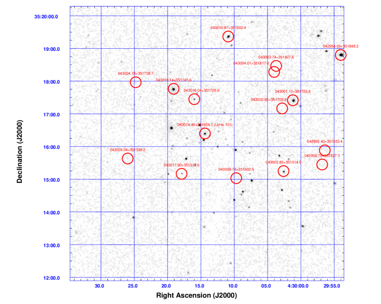
Figure 1: Close-up of the portion of the X-ray image also covered by the VLA field of view. The locations of the 16 radio sources considered in this paper are indicated with red circles. Radio sources have the prefix LkHa101VLA J prepended to the positions.

The VLA source positions were searched against the IRAC point source catalog (from Paper II) for matches. An offset of 1^′′ produced a total of 7 matches; relaxing the required positional coincidence to as much as 4 ^′′ did not produce any additional matches. Of these, 4 are Class III objects, 2 are Class II objects, and one (the central star LkH$\alpha$ 101) is classed as unknown. The VLA source positions were also cross-correlated against the Chandra source positions, with a positional coincidence of 1^′′ allowed for X-ray sources within 200^′′ of the pointing center, and 2.5^′′ allowed for X-ray sources greater than 200^′′ from the pointing center. Within 5^′ of LkH$\alpha$101, there are 132 X-ray sources, with 100 having counterparts in the IR catalog, 2 being Class I, 35 being Class II, 40 being Class III, and 23 being of unknown type. Figure 1 shows the portion of the Chandra image covered by the VLA field, with positions of radio sources indicated. Using the analytic expressions in Gehrels (1986) for the 1 $\sigma$ confidence limits for small numbers of events in Poisson statistics, the rate of radio emission for X-ray-emitting Class II objects is 2/35 or 6${}^{+7}_{-4}$%, and for Class III objects it is 4/40 or 10${}^{+8}_{-5}$%. We also searched the tables of Herbig et al. (2004) for correspondences with radio sources. The identification of the radio sources at other wavelengths is given in Table 2.

The radio observations reported on the sources around LkH$\alpha$101 span $\sim$20 years with the VLA, taken at different frequencies and configurations. Because several sources have reported flux densities at only one epoch, and because we expect variability to be a key characteristic of some of these sources, we extracted the previous epochs from the VLA archive, reduced, calibrated and imaged the data, and fitted Gaussians at the reported positions of all sources. We reproduced three out of the four epochs reported in BW88, as the fourth epoch (reported to have occurred on 1986 May 12) was not in NRAO’s on-line archive. We found different flux densities for [BW88] 7 and 8 on 1986 April 25: our fitted flux density for source 7 was consistent with that reported in BW88 for source 8, and vice versa. This may be the result of typographical error. We could not recover the new sources which were described in SO98 with our evaluation of the archival data. Although fluxes at $>$3$\sigma$ uncertainty were determined at these positions in other epochs, the unrecoverability of the sources along with absence of supporting data at other wavelengths led us to exclude the SO98 sources from consideration in subsequent analyses. Table 1 lists the flux densities for sources as reported in BW88, SO98, and by combining the data from our two days of observations.

The estimated number of foreground X-ray sources is small, and should not contaminate the sample of X-ray and radio coincidences. Our limiting X-ray sensitivity is about 10${}^{-15}~{}{\rm ergs}~{}{\rm cm}^{-2}~{}{\rm s}^{-1}$ in the 0.5-2.0 keV band (§3.5). The results from the Champlane (Hong et al., 2005) survey for $Chandra$ fields in the plane of the Galaxy but away from the galactic core indicate that we can expect to find about 70 background AGN, cataclysmic variables, neutron stars, black holes, and other non–PMS star point sources in a sample of 15 ACIS observations in the galactic plane, but not pointed at the galactic center, $(90^{\rm o}<l<270^{\rm o})$, sensitive to similar flux levels as we have. The number is most likely lower than this due to the nearly opaque nature of the dust clouds in the central $\sim$40% of the field, perhaps 45 total, or only $\sim$4 X-ray non-PMS point sources scaled to the 5 ^′overlap between the $Chandra$ field and the VLA 3.6 cm field, or a contamination of only 3% of the X-ray sources. Many of these are among the faint X-ray sources, X-ray sources with no optical/IR counterparts or the sources with offset between the X-ray position and optical/IR position exceeding 4^′′.

It is unlikely that the radio sources lacking X-ray and IR/optical counterparts are foreground sources. As discussed in §3.2, most of these objects have negative radio spectral indices, indicating nonthermal emission. Galactic sources of nonthermal radio emission should also produce nonthermal X-ray emission at a level above our detection limit (see §3.5); the lack of X-ray detection implies a ratio of X-ray to radio flux less than $\approx$6$\times$10¹¹ Hz. The lack of infrared or optical counterparts also constrains the presence of possible thermal radio sources; as discussed in the following paragraph, the Spitzer maps are sensitive to cluster members near the substellar mass limit, and foreground stellar objects will be brighter. In order to produce thermal emission at radio wavelengths but faint optical light a distance modulus that would place the objects beyond the cluster (and therefore not a foreground object) would be needed. Additionally, the space density of galactic foreground objects capable of being radio-bright but optical or X-ray faint is small enough that within the 5^′ radius of LkH$\alpha$101 we do not expect to see any of these sources.

We estimate the upper limit on IR magnitude for an object not to be detected in the IRAC bands, using the background levels due to nebulosity at the positions of the radio sources. We searched for the faintest star within 36^′′ of the position of each radio source not having an IR detection, and grouped sources with similar amounts of background. We find typical limits in JHK of 17, 15.5, and 15.3, respectively. At a distance modulus of 9.225, a $K_{mag}$ of 15.3 corresponds roughly to an absolute K magnitude of $\sim$6. According to Siess et al. (2000) a 1MY star with 0.1 M_⊙ would have a K_abs=4.39. DUSTY models (Chabrier et al., 2000; Baraffe et al., 2002) predict K_abs=6 for a 0.06 M_⊙ star, near the stellar-substellar boundary. Thus, the lack of an IR counterpart to apparent cluster members which are detected at other wavelengths may indicate that the object is a very low mass star or brown dwarf.

Eight of the radio sources considered here remain without a counterpart at X-ray or IR wavelengths. The reliability of these sources can be examined by the number of epochs or frequences at which each source has been detected. These eight sources have each been detected at more than one frequency or epoch; one source (LkHa101 J043004.0+351817) was identified in our observations at a single frequency on both days, as well as being marginally detected in the archival data from 1985 April (see Table 1). All of these sources are detected at $>$5 $\sigma$. Several of these are possible extragalactic sources. Becker & White (1988) identified their source [BW88] 5 as an extragalactic double. A check of the NRAO VLA Sky Survey (Condon et al., 1998) reveals three sources near LkH$\alpha$ 101 which are coincident (to less than 10”) with sources [BW88] 7, [BW88] 5, and [BW88] 2. As the integrated flux densities of these NVSS sources at 20 cm are 5.5, 4.1, and 3 mJy, respectively, which are all higher than the range of flux densities reported at the higher frequencies considered here, it is likely that these are extragalactic sources with steep radio spectral indices. The lack of coincidence with X-ray or IR sources supports this conjecture. Using a model for the 1.4 GHz extragalactic source counts, and converting from 1.4 GHz to 8.4 GHz using a spectral index of $\alpha$=-0.7, 5${}_{-2}^{+3}$ sources are expected in a circle of diameter 5.3’ with flux density greater than the 3 $\sigma$ rms at 8.4 GHz of 36 $\mu$Jy (J. Condon, private communication). This is consistent with all 8 radio sources lacking a counterpart at other wavelengths being extragalactic in nature.

3.2 Radio Spectral Index Measurements

The parameter which describes the shape of continuum radio emission is the spectral index $\alpha$, defined as $S_{\nu}\propto\nu^{\alpha}$; generally, for $\alpha\geq$ 0.5 the spectrum is rising, for $\alpha\leq-0.5$ the spectrum is falling, and in between ($-0.5\leq\alpha\leq 0.5$) the spectrum is considered flat. Rising spectra can generally be associated with optically thick thermal emission, falling spectra with optically thin nonthermal emission. Flat spectra could, in principle, be associated with either, but usually indicate nonthermal emission from an inhomogeneous source. Most of the sources for which spectral index constraints are available indicate negative spectral indices and consequently a nonthermal interpretation. Table 1 lists the spectral index derived from maps made by combining the two days of radio observations reported here; 13 objects have constraints on spectral index from detection at one or more frequencies. Eight of the 13 have spectral indices which are flat and slightly negative ($-0.8\leq\alpha\leq-0.1$); two are steeply negative ($\alpha\leq-1$); another two have large positive spectral indexes, one of which is the central star to the cluster, LkH$\alpha$101, and the other is a newly discovered source. Based on the multi-wavelength source identifications discussed in § 3.1, four objects with IR or X-ray detections have spectral index constraints, and 3/4 of these have negative spectral indices. Out of three objects with IR detections and spectral index constraints, two have negative spectral indices, one being a Class II object and the other a Class III object. Table 3 lists the spectral index measurements on each day. These are generally consistent with the values determined from the combined maps. The discrepant sources appear to have varied more at one wavelength than at the other. This behavior is discussed more in section 3.4.

3.3 Radio Variability

3.3.1 Long Timescale Radio Variability

In order to assess long-term radio variability, we considered the five epochs of 6 cm observations. We determined an object’s variability over the timescale of $\sim$ 20 years by examining the range of recorded flux values (including epochs where only upper limits were obtained) and determining how many $\sigma$ this range represents, using the largest measurement error. Flux determination can be affected by the beam size (if the object is slightly resolved), distance from the phase center, and contribution of background nebulosity. Since the observations were made in different array configurations, we place a conservative limit of 10$\sigma$ on the range of maximum to minimum flux values to assess variability. Using this criterion, 4 out of 9 sources can be considered variable; for objects detected on 4 or more occasions, only two can be considered variable. Table 4 lists the range of maximum to minimum variations in units of $\sigma$ for the 9 objects detected on one or more occasions at 6 cm.

3.3.2 Two-Day Radio Variability

We examined variations of the radio sources for changes between the two days of our recent observations. Table 3 lists the fluxes and spectral indices determined for each day and frequency. For all objects with at least one detection in our four intra-epoch maps (2 frequencies x 2 days), we examined the flux densities and error bars of each day to determination if there was statistical evidence for variability between the two days; we considered a source variable at one frequency if the two flux density measurements differed by more than 3$\sigma$, where the $\sigma$ of both flux density measurements was used. If an object was undetected on one day but detected on the other, it was considered variable if the detected flux was more than 3$\sigma$ above the upper limit. These results are recorded in Table 4. Using these criteria, 4 objects are considered variable at X-band, and 6 objects are considered variable at C-band.

3.3.3 Short Timescale Radio Variability

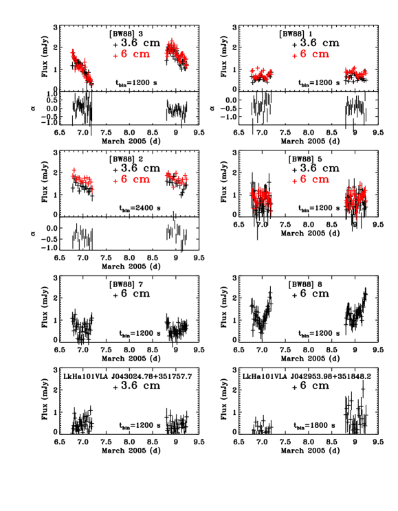
Figure 2: Short-term variability amongst the strongest radio sources. For objects where multi-frequency information is available and the individual flux measurements are strong enough, the time variation of the spectral index is plotted.

For radio sources with strong detections ($>10\sigma$) in the combined maps, we explored variability on time scales shorter than the 11 hour integrations each day. In order to do this, we subtracted the visibilities of all other sources from the calibrated visibility dataset, producing a dataset containing visibilities from only the target of interest. We imaged the result to ensure that no additional flux contribution from the other sources was present. We then searched for time variations in the visibility data using the AIPS task $DFTPL$, with offset fixed to the position of the source, and $uv$ distances restricted to the values used in imaging. We do not include in this analysis the radio-bright central object LkH$\alpha$ 101, due to its immersion in the extended H II emission region as well as the central ionized wind (imaged at higher frequencies in Gibb & Hoare, 2007), which makes it difficult to remove the visibilities of the extended emission. Also, based on its large positive spectral index, indicative of a thermal wind source, we do not expect to see variations in the flux density on such timescales. The daily averaged flux densities listed in Table 3 were measured from an image which had been corrected for the effects of the primary beam, while the visibility datasets used to measure short-timescale flux density variations do not include the effect of the primary beam. In order to compare the daily-averaged flux densities with the variations on shorter time-scales, we scaled the light curve flux densities by the primary-beam-corrected flux densities so that the average flux density from the light curve on each day matched the value in Table 3. Four sources were strong enough at both 3.6 and 6 cm to enable this; additionally, there were two sources which were only detected at 6 cm due to the larger field size, and one source with a stronger detection at 3.6 cm than at 6 cm. A final source was only detected on one day at one frequency. This selection resulted in 12 light curves, which are displayed in Figure 2. We made trial light curves using a number of different sized time bins, to explore evidence for variability given signal-to-noise constraints.

In order to asses evidence for variability from these light curves, we computed the average and standard deviation of the light curve flux values, determining the $\chi^{2}_{\nu}$ statistic and associated probability for variations about the average value. We also computed the distribution of fluxes and compared that with a Gaussian distribution with the same mean and standard deviation as the data. We computed the $\chi^{2}_{\nu}$ value between these two distributions as another measure of how the data depart from an expected constant value with scatter. Table 4 lists the probability that the observed $\chi^{2}_{\nu}$ statistic could be exceeded by a random variable for each of these two methods of assessing variability. We considered there to be evidence for short-term variability if both of these methods had probabilities of 5% or less. This resulted in two out of five objects showing evidence for variability at 3.6 cm, and four out of seven objects at 6 cm.

In addition,we also searched for statistically significant amounts of circularly polarized flux which might appear transiently during any flare activity, but not be statistically significant in the combined image. Our examination of the variation of Stokes V flux at the position of each of the target sources did not reveal any evidence for transient amounts of Stokes V flux.

3.4 Radio Variability and Spectral Index Changes

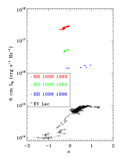
Figure 3: (left) Plot of 6 cm radio luminosity against 6–3.6 cm spectral index, for three objects for which changes in spectral index could be measured. Open squares indicate data points from the first day of observations, while the filled circles denote data from the second observation. The two apparent cluster members, [BW88] 1 and [BW88] 3, display a statistically significant anti-correlation between luminosity and spectral index, while the probable AGN ([BW88] 2) shows no correlation. (right) Plot displaying 6 cm radio luminosity against 6–3.6 cm spectral index for the decays of several radio flares from nearby active stars. Data for decays of radio flares from HR 1099 are taken from Osten et al. (2004); data for decay of radio flare from EV Lac is taken from Osten et al. (2005). The radio luminosities are positively correlated with spectral index over a wide range of luminosity.

The panels in Figure 2 show the temporal variation of spectral index for three objects with large enough flux density at both frequencies to permit determination of changes in the spectral index. [BW88] 3 is the only source where a large variation in flux density appears to be occurring during our observation. The light curve of [BW88] 1 also shows some short time-scale variability predominantly at 6 cm which also reveals itself as large negative values of $\alpha$. The behavior of radio luminosity versus spectral index is displayed in Figure 3 for the three objects in which spectral index changes can be discerned. The anti-correlation between luminosity and spectral index is statistically significant for sources [BW88] 3 and [BW88] 1 at the $>$99.9% level. In addition, we investigated the behavior between luminosity and spectral index for each day separately, as the light curves indicate differing amounts of variability on each day. For [BW88] 3, the anti-correlation is significant only at the 87% level on the first day (March 6), despite the obvious large-scale flux variations, and is not statistically significant on the second day (March 8). For [BW88] 1, the anti-correlation was significant at $>$99.7% and 90%, respectively, for the two days. For [BW88] 2, there was no correlation between radio luminosity and spectral index.

3.5 X-ray Fluxes

Our X-ray spectral fitting procedure is discussed in detail in Paper II and follows closely our previous work (Wolk et al., 2006, 2008). Spectra were fitted to about 100 sources with over 30 counts using several models for emission spectra from thermal, diffuse gas including that of Raymond & Smith (1977), Smith et al. (2001) and mekal (Mewe et al., 1985). In summary, in Paper II we find in the LkH$\alpha$ 101 cluster that the mean temperature of the coronae is about 2.5 keV, with the typical range between 800 eV and 5 keV. There were however 25 sources with temperatures $>$ 10 keV which were excluded from this analysis due to the low collecting area of the $Chandra$ HRMA. Typical $N_{\rm H}$ values ranged from 0-4 $\times 10^{22}$ cm^-2 with an outlier rejected mean of about 7.8 $\times 10^{21}$ cm^-2.

The spectroscopically measured absorbed fluxes range from 4.73$\times 10^{-13}$ to $4.89\times 10^{-15}$ erg cm^-2 sec^-1. Assuming a distance of 700 pc and correcting the measured X-ray absorption this becomes a luminosity range of about $log~{}L_{X}=29.75-31.64$ erg sec^-1. We compute the on-axis X-ray detection limits for a 3$\times 10^{7}$K plasma (kT$\sim$ 2.5 keV) with absorbing column density $\log N_{H}=$21.9 near the center of the field, and require 5 photons for a detection. The minimum absorbed flux is 6.2$\times$10^-16 erg cm^-2 s^-1, or $log~{}L_{X}\sim 28.5$ erg sec^-1for $d=700$ pc. This value is intended to give a rough sense of the sensitivity of the observation; variable absorption has a strong influence on the luminosity limit, as does off-axis distance. About twice the noted flux is required 4^′ off-axis.

3.6 X-ray Variability

X-ray variability of the sources in this field is discussed more thoroughly in the companion paper. Two independent analysis methods were used. First was a Bayesian block analysis which is common in the X-ray literature (BBs; Scargle, 1998; Getman et al., 2005; Wolk et al., 2006). For the Bayesian analysis we used two different priors, one prior was set to find variability at about 95% confidence and the second was set to 99.9% confidence. We also analyized the lightcurves following the method of Gregory & Loredo (1992, GL-vary). This method also uses Bayesian statistics and evaluates a large number of possible break points from the prediction of constancy. The advantage of the GL-vary method is that it handles data gaps and changes to the effective area well. It also calculates the odds that a source was constant. Thus, the analysis returns the probability that the source was variable and an estimate of the constant intervals within the observing window. All analyses were repeated on the data from the individual observations. We compare the results of Bayesian analysis with those of the more standard KS test by using the Chandra Orion Ultradeep Project (COUP) dataset (Getman et al., 2005) as an example: the BB algorithm found 973 variables, 95% of these were considered variable by the KS test at more than 99.9 % probability.

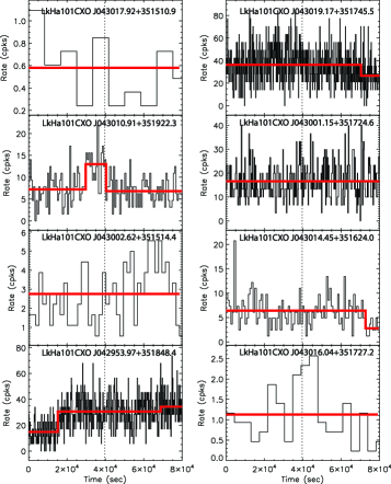
Figure 4: $Chandra$ light curves of radio-detected sources. The vertical line represents the break between the first observations, (ObsID 5429; 6 Mar 2005) and the second (ObsID 5428; 8 Mar 2005). The time histogram is binned so that the average bin contains 5 counts. Hence they range from about 100 seconds to about 9 ks in length. The red lines indicate intervals of constant flux as determined by Bayesian analysis set to detect variability at $>$ 95% confidence. IAU designators for source names are used. Count rate is counts per kilosecond.

For the purposes of this paper we consider only the eight X-ray sources with radio counterparts. The lightcurves for these sources are shown in Figure 4. Half of the sources show variability at $>95\%$ confidence based on the GL-vary method (sources LkHa101CXO J043019.2+351745, LkHa101CXO J043010.9+351922, LkHa101CXO J043002.6+351514 and LkHa101CXO J042954.0+351848). However no flaring or variations greather than a factor of two were seen. In fact, all of the sources seemed very stable between the two observations. The fact that no flares were seen is not particularly remarkable. The product of the observing time and the number of sources is about 640 ksec. This is about the mean time between macroscopic flares seen in young clusters (c.f. Wolk et al., 2005, 2006; Caramazza et al., 2007).

4 Results

These deep X-ray and radio observations probe multi-wavelength signatures of magnetic activity from the stars in the LkH$\alpha$ 101 star forming region. This paper focuses on the radio sources and associated multi-wavelength data and what we can learn about magnetic activity in these young stellar objects. There are three facets to the study described in this paper: the nature of the radio emitting sources, the variability of magnetic activity, and correlations between radio and X-rays, which we describe in the next sections.

4.1 On the Nature of the Radio-Emitting Cluster Members

Out of the 16 radio sources considered here, 8 are X-ray sources and 7 have Spitzer counterparts. There is a large overlap between radio-detected X-ray sources and radio-detected Spitzer sources: all of the IRAC sources are X-ray sources. The combination of X-ray and infrared detections bolsters support for these radio-emitting objects to be cluster members. Their close distance to the cluster center, and X-ray and infrared properties also make these objects consistent with being cluster members. In the following subsections, we provide a brief summary of the characteristics determined for each radio-emitting cluster member. The multi-wavelength identifications are summarized in Table 2.

4.1.1 LkHa101VLA J043017.90+351510.0 = [BW88] 1

[BW88] 1 was detected in the radio and X-ray maps, but does not have a detection in the Spitzer maps. There are no 2MASS point sources within 17” of the position of [BW88] 1 (Skrutskie et al., 2006). It is located in a region of high nebulosity, hence the infrared detection threshold requires about an additional magnitude compared to clear regions. Nonetheless, based on the upper limits in the Spitzer bands, if this object is a bona-fide member of the cluster, then it may be close to the substellar limit.

This is a bright and persistent radio source, detected on 5 out of 5 occasions (Table 1). Our simultaneous observations at 3.6 and 6 cm reveal a negative spectral index, suggesting nonthermal emission. This source shows no variability at radio wavelengths over the $\sim$20 years spanning the archival data and our data, but does appear to be variable at $>$ 3 $\sigma$ during the two days of our observations at C band (but not X band), and on shorter timescales at both wavelengths. The X-ray observations reveal no evidence of variability. The multi-frequency radio observations show an anti-correlation between radio flux density and spectral index. This object also displays a value of radio to X-ray luminosity more than 10 times that of other cluster members (§4.3). If this is a substellar object, the anomalously high ratio of its radio to X-ray luminosity when compared to the values found for the other stellar objects would fit with the few nearby field very low mass stars which display large radio luminosities relative to their X-ray luminosities (Berger, 2006).

4.1.2 LkHa101VLA J043019.14+351745.6 = [BW88] 3

[BW88] 3 has been detected in the radio, X-ray, and Spitzer maps, and is a Class II object based on its IR colors. Herbig et al. (2004) identified this source as a K0V star.

At radio wavelengths it is a persistent source, having been detected on 6/6 occasions, with a negative radio spectral index. The source shows large flux variations over the longest timescales probed here, and is variable over the two days in the most recent epoch at both X & C bands; it also displays variability on the shortest timescales, with a factor of 6 contrast between the highest/lowest flux densities. The large-scale short-term radio variability observed at 3.6 and 6 cm could be radio flares or rotational modulation. If rotational modulation, this would imply a likely period of $\approx$ 1–2 days and could arise from either geometrical effects or, alternatively, some form of directivity of the emission, similar to what has been seen in radio observations of the pre-main sequence star AB Doradus (Lim et al., 1994). Such an interpretation might imply that the emitting particles are much higher in energy than usually assumed for gyrosynchrotron emission. The radio observations on short timescales show an anti-correlation between radio flux density and spectral index, similar to that seen in [BW88] 1. There is statistical evidence for X-ray variability but no obvious X-ray flaring.

4.1.3 LkHa101VLA J043010.87+351922.4 = [BW88] 4

[BW88] 4 was detected at radio, X-ray, and IR wavelengths, and is a Class III object based on its IR colors. Becker & White (1988) argue that this is an obscured B dwarf, noting a small H II region around it.

At radio wavelengths [BW88] 4 has only been detected on 2 occasions out of 5, and only at C band, with a factor of $\approx$ 7 difference between the recorded flux densities. While this demonstrates large long-term radio variability, there are no significant variations over the shorter timescales probed by the two days of our observations. We have no constraints on radio spectral index. Multiple Bayesian blocks indicate X-ray variability on the first day.

4.1.4 LkHa101VLA J043001.15+351724.6 = [BW88] 6

[BW88] 6 has been detected at radio, X-ray, and IR wavelengths, and is a Class III object based on its IR colors. It has been identified by Herbig et al. (2004) as a K7 dwarf with Lithium. At radio wavelengths, it has been detected on 3 out of 6 occasions, with factor of $>$10 variability in two C-band detections. In our radio observations the object was detected only by summing all data from our two days’ integration at C band, so we have no constraints on shorter timescale variability, nor any constraint on spectral index. There is also no evidence for X-ray variability.

4.1.5 LkHa101VLA J043002.64+351514.9 = [BW88] 9

[BW88] 9 was detected in previous radio observations, and is detected in X-ray and Spitzer maps, with a Class II designation based on its IR colors. There is no spectral type for this object. It is only an intermittent radio source, having been detected on 2 out of 6 occasions at radio wavelengths. There is statistical evidence for X-ray variability but no large-scale flares.

4.1.6 LkHa101VLA J043014.43+351624.1 = LkH$\alpha$101

LkH$\alpha$101 is the source of the reflection nebula and H II region seen in optical/IR and radio images, and is also the source of a strong stellar wind. It has been detected at radio, X-ray, and IR wavelengths. The IR class is unknown due to the large amount of nebulosity, but observations at other wavelengths show the presence of a secondary as well as a face-on disk (Tuthill et al., 2001, 2002). The radio spectral index is large and positive, consistent with being a wind source. There is apparent variability between the X and C band flux densities measured on the two days, but this is likely not intrinsic to the source. There is no evidence for X-ray variability.

4.1.7 LkHa101VLA J042953.98+351848.2

This is a newly detected radio source, which has X-ray and IR counterparts, and based on its IR colors it is a class III object. No spectral type is known. This object was only detected at C band due to the wider full-width half power beam size, and was only detected on the second day of radio observations. It thus indicates radio variability between the two days as well as short-term radio variability. There is statistical evidence for X-ray variability and multiple Bayesian blocks on the first day of X-ray observations, but no variability on the second day when it is detected at radio wavelengths.

4.1.8 LkHa101VLA J043016.04+351726.9

This is another newly detected radio source, which has X-ray and IR counterparts, and is a class III object based on its IR colors. It has a spectral type of dM2 according to Herbig et al. (2004) and a flat or slightly negative radio spectral index. There is radio variability at C band over the two days with factor of two variations, but none at X band. There is no evidence for X-ray variability.

4.2 Variability and Magnetic Activity

4.2.1 Timescales of Magnetic Activity at Radio Wavelengths

There are three different timescales which we have explored for evidence of radio variability, and we find that roughly half the objects examined on each timescale are variable. Extragalactic objects could be radio variable due to AGN activity or interstellar scintillation, while cluster members could have variable radio emission due to magnetic activity. On the longest timescales of 20+ years, 4/9 sources with detections at 6 cm had more than 10$\sigma$ variations between the maximum recorded flux and the minimum or upper limit of recorded flux. Two of these sources appear to be cluster members. On the scale of days, 5/9 sources at 3.6 cm and 6/14 sources at 6 cm varied by more than 3$\sigma$, with two of the 5 variable sources at 3.6 cm being cluster members and 5 of the 6 variable sources at 6 cm being cluster members based on multi-wavelength identifications. On the smallest timescales of 1200–2400 s, 2/5 sources at 3.6 cm and 4/7 sources at 6 cm had a $>$ 95% probability of being variable; two of the variable sources at 3.6 cm and 6 cm are cluster members.

If we restrict ourselves to objects with counterparts at X-ray or IR wavelengths and thus probable cluster members, then 2/5 cluster members show evidence of variability on the longest timescales, 1/3 and 4/5 show day-to-day variations of more than 3 $\sigma$ at 3.6 and 6 cm, respectively, and 2/2 and 2/3 cluster members had a $>$95% probability of being variable on the shortest timescales at 3.6 and 6 cm, respectively. The small number of objects prevents a conclusive statistical analysis of whether cluster members are more likely to be radio variable than the background extragalactic objects. Four of the 8 sources detected at both radio and X-ray wavelengths showed evidence of being X-ray variable, despite lacking large-scale flares or factors of 2 or more variability. On the shortest timescales, radio variability appears to be a more common feature of cluster members than is X-ray variability.

4.2.2 Rapid Radio Variability

The radio observations on the shortest timescales reveal evidence of statistically significant flux changes in the majority of cluster members for which such measurements are possible. While the radio variability between the two days could be due to the contribution of different magnetic structures, the rapid radio variability is likely due to magnetic reconnection. The timescales for the rapid radio variability span from $>$ t_bin of 1200–2400 seconds to $\sim$ 11 hours, the duration of the large flux density enhancement seen in [BW88] 3. If we interpret these rapid variations as magnetic reconnection flaring, the timescale of the rapid radio variability argues for a low density environment. The Coulomb deflection times for particles of energy $E_{\rm kev}$ in a magnetic trap with ambient density $n_{e}$ cm^-3,

$$t_{\rm d}=0.8\frac{E_{\rm kev}^{3/2}}{(n_{e}/10^{8})}\frac{20}{\log\Lambda}\;\;\;s$$ (1)

where $\Lambda$ is the Coulomb logarithm (evaluated at the mean cluster temperature of 2.5 keV), constrains $t_{\rm d}$ to be $\gtrsim$1200–2400 seconds (time binning of the shortest variations) and $\lesssim$ 11 hours (the timescale for large flux density variations). For a 20 keV electron, this will occur for a range roughly $10^{5}\lesssim n_{e}(cm^{-3})\lesssim 5\times 10^{6}$, and for a 200 keV electron $5\times 10^{6}\lesssim n_{e}(cm^{-3})\lesssim 2\times 10^{8}$. We note that quantitative analyses of the time-dependent radio flux spectrum have been done for RS CVn binaries (Chiuderi Drago & Franciosini, 1993) but not, to our knowledge, for the more complicated magnetic field geometries around young stars (Donati et al., 2007). Such low densities are to be contrasted with the ambient electron density in X-ray-emitting coronal material, which is generally much higher ($n_{e}\geq$10⁹ cm^-3; Jardine et al., 2006).

4.2.3 Rapid Radio Variability and Lack of Circular Polarization

The constraints on circular polarization from the maps made of all the data, described in §2.1, can be applied to the measured flux densities at 3.6 and 6 cm to constrain the amount of circular polarization. At 3.6 cm, the minimum and maximum values of flux density imply 3 $\sigma$ limits on the percent of circularly polarized flux $V/I$ of $<$2% and $<$ 29%, respectively, while at 6 cm the corresponding limits are $<$ 2% and $<$ 31%, respectively.

The high level of radio variability implies a rapid re-arrangement of magnetic fields, but the lack of circular polarization potentially places a constraint on the spatial distribution of magnetic fields. Orientation can affect the observed amount of circular polarization for large-scale magnetic structures (edge-on configurations reveal contributions from both hemispheres, leading to a net cancellation). Alternatively, a magnetic configuration with many small-scale structures would also lead to a small net value of circular polarization. Even when circular polarization is detected in young stellar objects, it is usually at a low level (2–4% in quiescence, up to $\sim$16% during flares; White et al., 1992). Our upper limits on circular polarization are thus only weakly constraining.

4.2.4 Anti-correlation Between Flux Density and Spectral Index

There are two cluster members showing rapid radio variability which have strong enough detections to allow investigation of temporal changes in spectral index ([BW88] 1 and [BW88] 3). The spectral indices are generally flat or negative, $\alpha\lesssim$0.5, indicating nonthermal emission from an inhomogeneous source. The anti-correlation between 6 cm radio luminosity and spectral index (§3.4) is opposite to that seen from solar flares and active stars (Benz, 1977; Mutel et al., 1987). This anti-correlation has also been observed previously in young stellar radio sources: Felli et al. (1993) noted that some of the radio sources in Orion had spectral index changes associated with flux density changes on timescales of weeks, with $\alpha$ becoming more negative when the flux density increases. During the decays of radio flares from nearby active stars the spectral index and flux are positively correlated. The right panel of Figure 3 displays the 6 cm radio luminosity versus 6–3.6 cm spectral index for 4 well-observed radio flares from the active binary HR 1099 and the dMe flare star EV Lac (Osten et al., 2004, 2005). The positive correlations between radio luminosity and spectral index for these flares are significant at $>$99.5% confidence. Thus the observed trends in the two young stellar objects discussed here reveal a divergent behavior from that exhibited in active stars.

A detailed modelling of the flux density and spectral index and their temporal variations is beyond the scope of this paper. Nevertheless, we can examine the observed trends to infer constraints on the evolution of the population of accelerated particles. For radio flares from active stars the positive correlation between flux density and spectral index is considered to be a consequence of spectral evolution of optically thick emission during the rise and peak phases of the flare, returning to optically thin values during the flare decay. Under optically thin conditions, the spectral index is a function of only the power-law index of the accelerated electrons. Specifically, $\alpha\sim 1.2-0.9\delta$ for $2\leq\delta\leq 7$ (Dulk, 1985). Thus, for active stars, the positive correlation between flux density and spectral index means that at the peak of the flare when the flux density is maximum, $\alpha$ is large, corresponding to small values of $\delta$ which implies a hard distribution. At further points in the flare decay, the flux density has declined, with consequent smaller values of $\alpha$ and larger values of $\delta$. This temporal evolution is towards a softer accelerated electron distribution, such as can happen when the most energetic electrons are depopulated from e.g. radiative losses in a high B field region (left panel, Figure 5).

The anti-correlation between the flux density and spectral index seen in two cluster members suggests a different scenario than what is observed for active stars. For [BW88] 3 the temporal evolution of the flux density on both days looks like the decay phase of two flares, yet when the flux density is maximum, the spectral index is at its smallest. The temporal variations of [BW88] 1 are not ordered in the same way, yet produce the same anti-correlation. A small spectral index, under the same optically thin conditions as assumed above, implies a large value of $\delta$, while the large $\alpha$ corresponding to smaller values of flux density implies a smaller value of $\delta$ (right panel, Figure 5). This evolution of the accelerated particle spectrum is from soft to hard, and is difficult to envision under standard conditions of energy losses. This implies that the hardest energy electrons are being repopulated. For [BW88] 3 this timescale is several hours, whereas for [BW88] 1 it is on the order of the time binning, $\sim$1200 seconds. The conditions present in [BW88] 1 thus argue for a rapid but sporadic particle acceleration, while those in [BW88] 3 argue for nearly continuous particle acceleration during the transient events seen.

4.3 Radio/X-ray Correlations

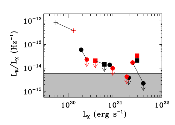
Figure 6: Ratio of radio to X-ray luminosities for radio sources considered in the present study. Black points indicate measurements on the first day (03/06), red points measurements obtained from the second day (03/08), and a line connects measurements of the same object. Class II objects are denoted by filled squares, while Class III objects have a filled circle for their data points. Data for the one object not detected with Spitzer are delineated by plus symbols. Down arrows indicate upper limits. The shaded curve indicates the region of $L_{X}-L_{R}$ space occupied by the GB relationship, with the order of magnitude uncertainty in the relationship, and constant appropriate to cTTs. It appears likely that these objects lie outside this relationship.

We investigated radio and X-ray luminosity correlations for objects detected at both radio and X-ray wavelengths, utilizing the simultaneously obtained measurements from our project. Figure 6 displays the results graphically, with X-ray and radio luminosity measurements taken from each of the two days of observations. We used a distance of 700 pc (Herbig et al., 2004), and the flux density measurements at 6 cm. The dotted lines connecting the pairs of points indicate the classification of the source using IRAC colors: there were 4 objects whose colors indicate photospheric levels, two whose colors were consistent with Class II sources, and one object not detected in the IRAC bandpass. We exclude the central object LkH$\alpha$101 from consideration, due to its early spectral type and the likelihood that the radio emission arises from an ionized wind. Two sources have only radio upper limits due to their nondetection at the current epoch, compared with detections at earlier epochs at levels up to five times the current upper limits. Also plotted is the expected range of X-ray and radio luminosities based on the observational relationship found by Güdel & Benz (1993, hereafter, GB). One might only expect the GB relationship to hold in wTTs but since we see that 1 cTTs displays nonthermal radio emission (see discusion in §3.2) we include the Class II objects as well.

Figure 6 indicates that the radio and X-ray luminosities displayed by these objects is not consistent with that implied by the GB relationship. For the Class II and III objects, there is considerable scatter in the measured values, with none of the radio and X-ray detections being consistent with the GB relationship (which would result in a ratio L_R/L_X of 5.9–59$\times$10^-16 Hz^-1 for wTTs). The prevalence of these objects above the GB relationship in the $L_{R}$-L_X plot indicates that they are more radio-luminous at a given X-ray luminosity than the GB relationship would imply. The sensitivity of our radio observations leads to a 5$\sigma$ constraint on radio luminosity of $\sim$6$\times$10¹⁶ erg s^-1 Hz^-1 for a source close to the phase center; based on arguments in §3.5 we estimated an X-ray sensitivity of $\sim$3$\times$10²⁸ erg s^-1 for an on-axis source at 700 pc distance. The X-ray sensitivity is capable of exploring a larger region of $L_{X}$-$L_{R}$ parameter space than is the current radio sensitivity. Note that two of our upper limits to radio luminosity could be consistent with the GB L_X-L_R relationship with radio observations $\approx$ 2–3 times more sensitive.

Magnetic fields are complicit in plasma heating which produces X-ray emission; magnetic fields also accelerate electrons and give rise to radio emission. It is natural, then, to assume that a relationship might hold between two observable sources of radiation whose formations require the presence of magnetic fields. Güdel & Benz (1993) argued that the two quantities can be roughly linearly related through conversion of coronal energy into plasma heating and X-ray radiation on the one hand, and particle acceleration and radio emission on the other hand. Another way the two quantities may be linearly related is if the radio- and X-ray-emitting volumes are co-spatial. But this places a stringent constraint on the X-ray-emitting plasma, because the radio radiation must be able to escape and be detected. Using parameters from the X-ray spectral fits to the integrated data for radio- and X-ray detected sources, and assuming a spherically symmetric corona with stellar radii of $\approx$ 2R_⊙, roughly appropriate for stars of about 1 Myr, we estimate the free-free optical depth of the X-ray emitting material at radio wavelengths (equation 11.2.2 in Benz, 2002) and find that the X-ray emitting material would be optically thick at radio wavelengths. This rules out co-spatial formation of X-ray and radio emission. To produce detectable quantities of radio and X-ray emission requires the presence of large scale magnetic fields and/or large amounts of magnetic flux. It is entirely possible that with a complex field geometry, X-ray and radio-emitting regions are physically distinct from each other, with separate energy reservoirs. If this is the case, no relationship between the two emergent intensities is to be expected.

Figure 6 displays the ratio of the luminosities against X-ray luminosity. There is a statistically significant anti-correlation between this luminosity ratio and the X-ray luminosity; the discrepancy between the observed luminosity ratio and that expected from the GB relationship grows as the X-ray luminosity decreases. It is likely that [BW88] 1, the most extreme object exhibiting this relationship, is a very low mass star or brown dwarf (see discussion in §3.1). The luminosity ratio relates the efficiency of particle acceleration (through the production of nonthermal radio emission) to that of plasma heating (through the production of X-ray emission). Although the GB relationship implies a nearly constant amount of particle acceleration relative to plasma heating, the results for the young stellar objects around LkH$\alpha$101 indicate that this parameter depends on the amount of plasma heating, and thus implies a decoupling of particle acceleration from plasma heating.

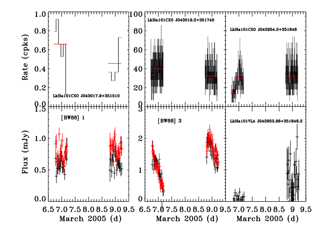
Figure 7: X-ray and radio light curves for three objects with radio fluxes high enough to examine short time-scale radio variability. Top panels: Chandra light curves as in Figure 4, bottom panels: radio light curves as in Figure 2. There is no apparent correlation between radio and X-ray variability in these objects.

The lack of correlation between radio and X-ray measurements can also be seen in the comparison of short time-scale variability: The amount of radio variability between the two days of observations is larger than the corresponding range in X-ray flux in the sample of objects detected at both wavelengths. Out of 8 sources detected at both X-ray and radio wavelengths, variability at both wavelengths is seen in only two cases ([BW88] 3, LkHa101VLA J0429540.+351848). Yet, two objects appeared to be undergoing short time-scale variability ([BW88] 3, [BW88] 1), while no X-ray flares were seen. The comparison of X-ray and radio variability is shown in Figure 7 for the three objects having significant radio detections, to probe variability in both. Variability appears to be a greater factor in the production of radio emission than it is in X-ray emission.

5 Discussion

There has been a paucity of simultaneous radio and X-ray observations of young stars, despite the large potential for learning about magnetic fields and interrelation of plasma heating and particle acceleration. The small number of cases in hand suggest a different scenario from that gleaned from studies of the Sun and nearby active stars. Simultaneous multi-wavelength observations of HD 283447 by Feigelson et al. (1994) revealed a radio flare but no X-ray or chromospheric variability. They concluded that the regions of gyrosynchrotron emission were largely decoupled from the regions where plasma heating was occurring. Bower et al. (2003) serendipitously observed a giant outburst at mm- wavelengths during the COUP observation; an intense X-ray flare on the same star began 3 days prior to the observed radio flare and lasted through the duration of the radio flare. Gagné et al. (2004) found a star, DoAr 21, in the $\rho$ Opch cloud core to be in the the decay phase of an X-ray flare with stable emission at 6 cm. These examples are opposite to the classic “Neupert effect” and suggestive of a different flare scenario. Time-averaged correlations also show a different behavior in young stellar objects. Gagné et al. (2004) found no evidence that X-ray and radio luminosities are correlated as expected in the GB relationship for a small sample of TTs in the $\rho$ Ophiucus cloud. Observations of Class I sources in the Coronet cluster (Forbrich et al., 2006, 2007) similarly show no clear correlations between radio and X-ray emission as should appear in the GB relationship if particle acceleration and plasma heating arise from a common energy reservoir. Our finding of a decoupling between radio and X-ray emission in both a time-averaged and time variable sense supports the idea that the structures giving rise to the two emissions in young stellar objects are physically or energetically distinct.

We find as a common theme that there is a different scenario for magnetic activity in the young stellar objects around LkH$\alpha$101 than is usually seen in the Sun and active stars. This is revealed by a comparison between radio flux versus spectral index behavior, which suggests for the young stellar objects studied here rapid particle acceleration and injection. The interpretation of the dependence of radio to X-ray luminosity ratio on X-ray luminosity is that the efficiency of particle acceleration relative to plasma heating depends on the amount of plasma heating, rather than being relatively independent as for active stars and the Sun. We investigated the coronal structures which could be giving rise to the radio and X-ray emission, and find several lines of evidence that such a decoupling is occurring. The X-ray emitting loops are optically thick to radio emission at the wavelengths observed, so the detected amounts of radio and X-ray emission can not be coming from co-spatial loops. The isolation of radio- and X-ray emitting material is also consistent with one interpretation of the lack of expected roughly linear correlation between X-ray and radio luminosities. The observed rapid radio variability implies a low density environment, another disconnect between the spatial location of radio emitting structures and X-ray emitting structures, as inferred X-ray densities are much higher.

We can also constrain the size scales of X-ray and radio emission. Since the observed X-ray luminosity is proportional to the volume emission measure (VEM), a function of the coronal electron density and size scale, for a spherically symmetric corona we have

$$VEM\propto\int n_{e}^{2}dV\sim 4\pi R_{\star}^{2}\int n_{e}^{2}ds$$ (2)

where R_⋆ is the stellar radius, which we take for YSOs to be roughly 2 (see discussion in §4.3). Using the observed X-ray luminosities and derived column emission measures in §4.3, combined with coronal density estimates of n_e between 0.6–2.5 $\times$10¹⁰ cm^-3 (Jardine et al., 2006), implies size scales for the X-ray emission of $l_{X}/R_{\star}$ between 0.002 and 2, and thus relatively compact. For gyrosynchrotron emission appearing at the observed radio frequencies, valid for harmonics of the gyrofrequency $\nu=s\nu_{B}$ for $s$ between 10 and 100 with $\nu_{B}$=2.8$\times$10⁶B Hz, the inferred magnetic field strengths in the region of radio emission are between 17 and 300 G. If we assume that this emission originates from a dipole field geometry, and the surface magnetic fields are in the range 1–3 kG (Johns-Krull, 2007), then the scale size of the radio emission $l_{R}$ is between 1.6 and 6 R_⋆. This shows that the radio emission appears to be physically distinct from the X-ray emission. This conclusion has also been reached by Feigelson et al. (1994) and Massi et al. (2006) for the case of HD 283447.

If there is a large-scale distribution of magnetic fields giving rise to the radio emission, the lack of circular polarization constrains the orientation of the emission to be largely edge-on, while a magnetic configuration composed of small-scale fields would also explain a null detection of circular polarization in radio emission. Recent magnetic field measurements in TTs show that strong and complex magnetic field geometries are present, which can potentially interfere with X-ray generation (Johns-Krull, 2007) and probably radio generation as well. Jardine et al. (2006) noted from modelling the X-ray emission of T Tauri stars that more complex field geometries were associated with more compact, denser coronae. Perhaps the complex field configuration and possible coupling of disk to star changes the emergent radiations associated with the magnetic fields in such a way as to break the $L_{x}-L_{r}$ relation and any variability correlations.

6 Conclusions

We find that nonthermal radio emission (based on flat/negative spectral indices) can be produced even in stars with infrared evidence for disks. In fact, we see large-scale radio emission variability from one Class II object ([BW88] 3), as well as a possibly substellar object ([BW88] 1). Thus radio emission can be used as a diagnostic of magnetic activity in young stellar objects both with and without disks. Using this observational tool, we find a variety of behaviors indicating a different kind of magnetic activity from that seen on active stars and the Sun: anti-correlation between radio luminosity and radio spectral index, lack of expected correlation between radio and X-ray luminosities, lack of correlated variability between radio and X-ray emission, and anti-correlation between the ratio of radio to X-ray luminosity and X-ray luminosity. The anti-correlation between radio flux and spectral index points to a gyrosynchrotron emission mechanism which requires a different evolution of field strength, number density of accelerated electrons, and distribution compared to what is seen on nearby active stars and the Sun. The multi-wavelength behaviors suggest a decoupling between particle acceleration and plasma heating, in both time-averaged and time-variable trends. The lack of expected correlation between radio and X-ray luminosities can be interpreted as due to their production in different magnetic regions, or out of different energy reservoirs. There are a few calculations which support the former: the different inferred electron densities for X-ray emitting material versus that required to explain the rapid variability of radio emission (X-ray emission arising from denser regions); the calculated optical depth to radio emission of the X-ray-emitting plasma (showing that the X-ray emitting plasma would be optically thick and therefore not likely to escape and be detected at radio wavelengths); and the lack of correspondence between estimated X-ray size scales and radio size scales, which suggest for simple configurations that the X-ray emission is more compact than the radio emission.

The primary finding of our investigation is that the magnetic activity signatures (radio, X-ray) and their correlations from young stellar objects in the LkH$\alpha$101 cluster show different trends from those established for nearby active stars. Our results are new in that we probe a region of variability space occupied by few other multi-wavelength observations of young stellar objects: long-duration, multi-frequency radio coverage, with simultaneous multi-wavelength observations. We conclude that we are likely seeing evidence of a new phenomenon in these highly active young stars. Our conclusions are tempered by the small number of objects in our analysis, which is a result of the asymmetry between percentages of radio and X-ray emission in cluster members. We are expanding our multi-wavelength investigation in magnetic activity from young stars with current and future observations of clusters spanning a range in ages. The simultaneous multi-wavelength coverage in this campaign was vital to establishing the disconnect between these magnetic activity signatures, and points out the parameter space available for future such studies. Future observations with the Expanded Very Large Array (EVLA), with roughly a factor of ten increase in sensitivity to radio emission, will be able to expand upon the findings presented here.

Table 1: Long-term Behavior of Radio Sources in the Field around LkH $\alpha$101

ID	April 1985	January 1986	April 1986	May 1986	October 1991	March 2005	March 2005	$\alpha$
	6 cm	6 cm	6 cm	6 cm	3.6 cm	3.6 cm	6 cm
LkHa101VLA J043017.90+351510.0	0.7$\pm$0.1	1.1$\pm$0.1	1.0$\pm$0.2	NI	0.63$\pm$0.07	0.629$\pm$0.013	0.794$\pm$0.016	-0.43$\pm$0.05
LkHa101VLA J043026.04+351538.2	2.0$\pm$0.1	2.2$\pm$0.1	2.1$\pm$0.2	1.4$\pm$0.1	1.65$\pm$0.12	1.428$\pm$0.016	1.694$\pm$0.019	-0.32$\pm$0.03
LkHa101VLA J043019.14+351745.6	2.9$\pm$0.1	1.2$\pm$0.1	2.2$\pm$0.1	4.2$\pm$0.2	1.12$\pm$0.11	1.276$\pm$0.014	1.347$\pm$0.018	-0.10$\pm$0.03
LkHa101VLA J043010.87+351922.4	1.3$\pm$0.1	$<$0.1	$<$0.4	$<$0.2	OOF	OOF	0.222$\pm$0.023	–
LkHa101VLA J043003.74+351827.6	0.9$\pm$0.1	2.0$\pm$0.1	OOF	NI	0.46$\pm$0.07	0.616$\pm$0.018	0.832$\pm$0.021	-0.55$\pm$0.07
LkHa101VLA J043001.15+351724.6	0.5$\pm$0.1	$<$0.1	$<$0.4	$<$0.2	0.33$\pm$0.08	OOF	0.056$\pm$0.016	–
LkHa101VLA J042956.40+351553.4	1.2$\pm$0.1	1.8$\pm$0.1	$<$0.4	0.7$\pm$0.1	0.22$\pm$0.06	OOF	0.578$\pm$0.022	–
LkHa101VLA J042956.78+351527.1	0.5$\pm$0.1	0.8$\pm$0.1	1.1$\pm$0.2	0.6$\pm$0.1	0.50$\pm$0.06	OOF	1.249$\pm$0.025	–
LkHa101VLA J043002.64+351514.9	$<$0.2	0.8$\pm$0.1	$<$0.4	$<$0.2	0.81$\pm$0.10	$<$0.072	$<$0.059	–
LkHa101VLA J042958.00+351602.9	$<$0.3	$<$0.2	$<$0.3	NI	0.82$\pm$0.17	OOF	0.117$\pm$0.022	–
LkHa101VLA J043008.77+351625.8	$<$0.3	0.22$\pm$0.06	OOF	NI	1.05$\pm$0.14	$<$0.036	$<$0.036	–
LkHa101VLA J043010.98+351437.6	$<$0.3	$<$0.2	OOF	NI	0.29$\pm$0.05	0.058$\pm$0.014	$<$0.054	$>$0.2
LkHa101VLA J043014.43+351624.1	NI	NI	NI	NI	NI	38.134$\pm$0.011	24.643$\pm$0.014	0.805$\pm$0.001
LkHa101VLA J043014.46+351527.5	$<$0.3	$<$0.2	OOF	NI	0.38$\pm$0.06	$<$0.036	0.067$\pm$0.015	$<$-1
LkHa101VLA J043016.53+351710.8	$<$0.3	$<$0.2	OOF	NI	0.55$\pm$0.10	$<$0.036	$<$0.045	–
LkHa101VLA J043016.98+351642.4	$<$0.3	$<$0.2	OOF	NI	0.65$\pm$0.14	0.043$\pm$0.011	0.066$\pm$0.015	-0.8$\pm$0.6
LkHa101VLA J043017.34+351647.6	$<$0.3	$<$0.2	OOF	NI	0.54$\pm$0.08	0.103$\pm$0.012	0.063$\pm$0.015	0.9$\pm$0.4
LkHa101VLA J043009.74+351502.5	$<$0.3	$<$0.2	OOF	NI	$<$0.18	0.138$\pm$0.013	0.149$\pm$0.018	-0.1$\pm$0.3
LkHa101VLA J043002.85+351709.8	$<$0.3	$<$0.2	$<$0.3	NI	$<$0.3	0.129$\pm$0.016	0.171$\pm$0.018	-0.5$\pm$0.3
LkHa101VLA J043004.01+351817.0	0.36$\pm$0.12	$<$0.2	OOF	NI	$<$0.3	$<$0.054	0.227$\pm$0.020	$<$-3
LkHa101VLA J042953.98+351848.2	$<$0.3	$<$0.2	OOF	NI	OOF	OOF	0.353$\pm$0.027	–
LkHa101VLA J043016.04+351726.9	$<$0.3	$<$0.2	OOF	NI	$<$0.2	0.103$\pm$0.012	0.124$\pm$0.016	-0.4$\pm$0.3
LkHa101VLA J043024.78+351757.7	$<$0.4	$<$0.2	OOF	NI	OOF	0.323$\pm$0.016	0.223$\pm$0.021	0.6$\pm$0.2

Table 2: Multi-wavelength cross-identification of sources

Radio ID	other Radio ID	X-ray ID	IRAC counterpart	IR Class	spectral type
LkHa101VLA J043017.90+351510.0	[BW88] 1, [SO98] 12	LkHa101CXO J043017.9+351510
LkHa101VLA J043026.04+351538.2	[BW88] 2, [SO98] 14				probable AGN(see §4.1.2)
LkHa101VLA J043019.14+351745.6	[BW88] 3,[SO98] 13	LkHa101CXO J043019.2+351745	LkHa101SST J043019.16+351745.5	2	K0: (Herbig et al., 2004)
LkHa101VLA J043010.87+351922.4	[BW88] 4	LkHa101CXO J043010.9+351922	LkHa101SST J043010.89+351922.6	3	BV (BW88)
LkHa101VLA J043003.74+351827.6	[BW88] 5,[SO98] 4				probable AGN (see §4.1.2)
LkHa101VLA J043001.15+351724.6	[BW88] 6, [SO98] 16	LkHa101CXO J043001.1+351724	LkHa101SST J043001.13+351724.8	3	K7 (Herbig et al., 2004)
LkHa101VLA J042956.40+351553.4	[BW88] 7, [SO98] 15				probable AGN (see §4.1.2)
LkHa101VLA J042956.78+351527.1	[BW88] 8, [SO98] 1
LkHa101VLA J043002.64+351514.9	[BW88] 9, [SO98] 3	LkHa101CXO J043002.6+351514	LkHa101SST J043002.62+351514.4	2
LkHa101VLA J042958.00+351602.9	SO 2
LkHa101VLA J043008.77+351625.8	SO 5
LkHa101VLA J043010.98+351437.6	SO 6
LkHa101VLA J043014.43+351624.1	LkH$\alpha$101, SO 7	LkHa101CXO J043014.4+351624	LkHa101SST J043014.44+351624.0	100	early B; see discussion in Herbig et al. (2004)
LkHa101VLA J043014.46+351527.5	SO 8
LkHa101VLA J043016.53+351710.8	SO 9
LkHa101VLA J043016.98+351642.4	SO 10
LkHa101VLA J043017.34+351647.6	SO 11
LkHa101VLA J043009.74+351502.5
LkHa101VLA J043002.85+351709.8
LkHa101VLA J043004.01+351817.0
LkHa101VLA J042953.98+351848.2		LkHa101CXO J042954.0+351848	LkHa101SST J042953.97+351848.6	3
LkHa101VLA J043016.04+351726.9		LkHa101CXO J043016.0+351727	LkHa101SST J043016.04+351727.2	3	M2 (Herbig et al., 2004)
LkHa101VLA J043024.78+351757.7

Table 3: Two-Day Behavior of Radio Sources in the Field around LkH$\alpha$101

ID	$\theta$	03/06	03/06	03/08	03/08	$\alpha_{1}$	$\alpha_{2}$
	(”)	3.6 cm	6 cm	3.6 cm	6 cm
LkHa101VLA J043017.90+351510.0	84	0.614$\pm$0.018	0.760$\pm$0.021	0.639$\pm$0.018	0.831$\pm$0.021	-0.39$\pm$0.07	-0.48$\pm$0.07
LkHa101VLA J043026.04+351538.2	149	1.343$\pm$0.022	1.678$\pm$0.025	1.518$\pm$0.022	1.708$\pm$0.024	-0.41$\pm$0.04	-0.22$\pm$0.04
LkHa101VLA J043019.14+351745.6	102	0.9894$\pm$0.019	0.992$\pm$0.035	1.580$\pm$0.019	1.672$\pm$0.023	0$\pm$0.6	-0.10$\pm$0.03
LkHa101VLA J043010.87+351922.4	185	OOF	0.214$\pm$0.030	OOF	0.218$\pm$0.031	–	–
LkHa101VLA J043003.74+351827.6	181	0.636$\pm$0.025	0.850$\pm$0.028	0.590$\pm$0.026	0.813$\pm$0.028	-0.53$\pm$0.09	-0.6$\pm$0.1
LkHa101VLA J043001.15+351724.6	174	OOF	$<$0.072	OOF	$<$0.072	–
LkHa101VLA J042956.40+351553.4	222	OOF	0.625$\pm$0.030	OOF	0.562$\pm$0.029	–	–
LkHa101VLA J042956.78+351527.1	222	OOF	1.178$\pm$0.033	OOF	1.310$\pm$0.032	–	–
LkHa101VLA J043002.64+351514.9	159	$<$0.081	$<$0.081	$<$0.069	$<$0.081	–	–
LkHa101VLA J043014.43+351624	2	36.168$\pm$0.015	23.099$\pm$0.019	37.788$\pm$0.015	23.196$\pm$0.018	0.827$\pm$0.002	0.900$\pm$0.002
LkHa101VLA J043009.74+351502.5	98	0.084$\pm$0.017	0.113$\pm$0.022	0.183$\pm$0.019	0.148$\pm$0.022	-0.5$\pm$0.5	0.4$\pm$0.3
LkHa101VLA J043002.85+351709.8	149	0.139$\pm$0.021	0.167$\pm$0.044	0.124$\pm$0.022	0.149$\pm$0.024	-0.3$\pm$0.3	-0.4$\pm$0.4
LkHa101VLA J043004.01+351817.0	171	$<$0.072	0.171$\pm$0.024	$<$0.072	0.129$\pm$0.025	$<$-1.6	$<$-1
LkHa101VLA J042953.98+351848.2	289	OOF	$<$0.150	OOF	0.724$\pm$0.036	–	–
LkHa101VLA J043016.04+351726.9	68	0.135$\pm$0.017	0.188$\pm$0.021	0.125$\pm$0.017	0.093$\pm$0.020	-0.6$\pm$0.3	0.5$\pm$0.4
LkHa101VLA J043024.78+351757.7	159	0.405$\pm$0.023	0.232$\pm$0.029	0.282$\pm$0.022	0.201$\pm$0.026	1.2$\pm$0.2	0.6$\pm$0.3

Table 4: Variability Statistics

ID	Long Term Var.	2-day Var.	2-day Var.	Short Term Var.	Short Term Var.	PXR
	6 cm	3.6 cm	6 cm	3.6 cm	6 cm	(%)
LkHa101VLA J043017.90+351510.0	N	N	Y	Y	Y	60
LkHa101VLA J043026.04+351538.2	N	Y	N	N	N	-
LkHa101VLA J043019.14+351745.6	Y	Y	Y	Y	Y	97
LkHa101VLA J043010.87+351922.4	Y	-	N	-	-	95
LkHa101VLA J043003.74+351827.6	Y	N	N	N	Y	-
LkHa101VLA J043001.15+351724.6	N	-	-	-	-	17
LkHa101VLA J042956.40+351553.4	Y	-	N	-	N	-
LkHa101VLA J042956.78+351527.1	N	-	Y	-	Y	-
LkHa101VLA J043002.64+351514.9	N	-	-	-	-	99
LkHa101VLA J043014.43+351624.1	-	Y	Y	-	-	72
LkHa101VLA J043009.74+351502.5	-	Y	N	-	-	-
LkHa101VLA J043002.85+351709.8	-	N	N	-	-	-
LkHa101VLA J043004.01+351817.0	-	-	N	-	-	-
LkHa101VLA J042953.98+351848.2	-	-	Y	-	N	$>$99.9
LkHa101VLA J043016.04+351726.9	-	N	Y	-	-	82
LkHa101VLA J043024.78+351757.7	-	Y	N	N	-	-

Figure 5: (left) Schematic relationship between flux density and spectral index observed in the decay phase of flares on active stars. Solid vertical line in S_ν vs. $\alpha$ plot indicates $S_{\nu}$, $\alpha$ measurements at a time early in the flare decay, while dashed vertial line indicates $S_{\nu}$, $\alpha$ measurements at a later time in the flare decay. Solid slanted line in $N(E)$ vs. $E$ figure indicates relative distribution of accelerated particles at the time early in the flare decay, while slanted dashed line indicates that for later in the flare decay, based on the change of $\alpha$ under optically thin conditions. The interpretation of the decrease in $\alpha$ is a a softening of the accelerated electron population during the flare decay. (right) Schematic relationship between flux density and spectral index for two young stellar objects seen here and in Felli et al. (1993). Solid and dashed lines are the same as for the left panels. The hardening of the accelerated electron spectrum from early in the flare decay to later times implies sporadic or near-continuous acceleration of electrons to repopulate the distribution.

References

- André et al. (1987) André, P., Montmerle, T., & Feigelson, E. D. 1987, AJ, 93, 1182
- Aspin & Barsony (1994) Aspin, C. & Barsony, M. 1994, A&A, 288, 849
- Baraffe et al. (2002) Baraffe, I., Chabrier, G., Allard, F., & Hauschildt, P. H. 2002, A&A, 382, 563
- Barsony et al. (1990) Barsony, M., Scoville, N. Z., Schombert, J. M., & Claussen, M. J. 1990, ApJ, 362, 674
- Becker & White (1988) Becker, R. H. & White, R. L. 1988, ApJ, 324, 893
- Benz (2002) Benz, A., ed. 2002, Astrophysics and Space Science Library, Vol. 279, Plasma Astrophysics, second edition
- Benz (1977) Benz, A. O. 1977, ApJ, 211, 270
- Benz & Güdel (1994) Benz, A. O. & Güdel, M. 1994, A&A, 285, 621
- Berger (2006) Berger, E. 2006, ApJ, 648, 629
- Bieging et al. (1984) Bieging, J. H., Cohen, M., & Schwartz, P. R. 1984, ApJ, 282, 699
- Bower et al. (2003) Bower, G. C., Plambeck, R. L., Bolatto, A., McCrady, N., Graham, J. R., de Pater, I., Liu, M. C., & Baganoff, F. K. 2003, ApJ, 598, 1140
- Caramazza et al. (2007) Caramazza, M., Flaccomio, E., Micela, G., Reale, F., Wolk, S. J., & Feigelson, E. D. 2007, A&A, 471, 645
- Chabrier et al. (2000) Chabrier, G., Baraffe, I., Allard, F., & Hauschildt, P. 2000, ApJ, 542, 464
- Chabrier & Küker (2006) Chabrier, G. & Küker, M. 2006, A&A, 446, 1027
- Chiuderi Drago & Franciosini (1993) Chiuderi Drago, F. & Franciosini, E. 1993, ApJ, 410, 301
- Condon et al. (1998) Condon, J. J., Cotton, W. D., Greisen, E. W., Yin, Q. F., Perley, R. A., Taylor, G. B., & Broderick, J. J. 1998, AJ, 115, 1693
- Dobler et al. (2006) Dobler, W., Stix, M., & Brandenburg, A. 2006, ApJ, 638, 336
- Donati et al. (2007) Donati, J.-F., Jardine, M. M., Gregory, S. G., Petit, P., Bouvier, J., Dougados, C., Ménard, F., Cameron, A. C., Harries, T. J., Jeffers, S. V., & Paletou, F. 2007, MNRAS, 760
- Dulk (1985) Dulk, G. A. 1985, ARA&A, 23, 169
- Feigelson et al. (1998) Feigelson, E. D., Carkner, L., & Wilking, B. A. 1998, ApJ, 494, L215+
- Feigelson & Montmerle (1999) Feigelson, E. D. & Montmerle, T. 1999, ARA&A, 37, 363
- Feigelson et al. (1994) Feigelson, E. D., Welty, A. D., Imhoff, C., Hall, J. C., Etzel, P. B., Phillips, R. B., & Lonsdale, C. J. 1994, ApJ, 432, 373
- Felli et al. (1993) Felli, M., Taylor, G. B., Catarzi, M., Churchwell, E., & Kurtz, S. 1993, A&AS, 101, 127
- Fisher et al. (1985) Fisher, G. H., Canfield, R. C., & McClymont, A. N. 1985, ApJ, 289, 425
- Forbrich et al. (2006) Forbrich, J., Preibisch, T., & Menten, K. M. 2006, A&A, 446, 155
- Forbrich et al. (2007) Forbrich, J., Preibisch, T., Menten, K. M., Neuhäuser, R., Walter, F. M., Tamura, M., Matsunaga, N., Kusakabe, N., Nakajima, Y., Brandeker, A., Fornasier, S., Posselt, B., Tachihara, K., & Broeg, C. 2007, A&A, 464, 1003
- Gagné et al. (2004) Gagné, M., Skinner, S. L., & Daniel, K. J. 2004, ApJ, 613, 393
- Gehrels (1986) Gehrels, N. 1986, ApJ, 303, 336
- Getman et al. (2005) Getman, K. V., Flaccomio, E., Broos, P. S., Grosso, N., Tsujimoto, M., Townsley, L., Garmire, G. P., Kastner, J., Li, J., Harnden, Jr., F. R., Wolk, S., Murray, S. S., Lada, C. J., Muench, A. A., McCaughrean, M. J., Meeus, G., Damiani, F., Micela, G., Sciortino, S., Bally, J., Hillenbrand, L. A., Herbst, W., Preibisch, T., & Feigelson, E. D. 2005, ApJS, 160, 319
- Gibb & Hoare (2007) Gibb, A. G. & Hoare, M. G. 2007, MNRAS, 380, 246
- Gregory & Loredo (1992) Gregory, P. C. & Loredo, T. J. 1992, ApJ, 398, 146
- Güdel et al. (2002) Güdel, M., Audard, M., Smith, K. W., Behar, E., Beasley, A. J., & Mewe, R. 2002, ApJ, 577, 371
- Güdel & Benz (1993) Güdel, M. & Benz, A. O. 1993, ApJ, 405, L63
- Güdel et al. (1996) Güdel, M., Benz, A. O., Schmitt, J. H. M. M., & Skinner, S. L. 1996, ApJ, 471, 1002
- Hawley et al. (2003) Hawley, S. L., Allred, J. C., Johns-Krull, C. M., Fisher, G. H., Abbett, W. P., Alekseev, I., Avgoloupis, S. I., Deustua, S. E., Gunn, A., Seiradakis, J. H., Sirk, M. M., & Valenti, J. A. 2003, ApJ, 597, 535
- Herbig et al. (2004) Herbig, G. H., Andrews, S. M., & Dahm, S. E. 2004, AJ, 128, 1233
- Hong et al. (2005) Hong, J., van den Berg, M., Schlegel, E. M., Grindlay, J. E., Koenig, X., Laycock, S., & Zhao, P. 2005, ApJ, 635, 907
- Jardine et al. (2006) Jardine, M., Cameron, A. C., Donati, J.-F., Gregory, S. G., & Wood, K. 2006, MNRAS, 367, 917
- Johns-Krull (2007) Johns-Krull, C. M. 2007, ApJ, 664, 975
- Lim et al. (1994) Lim, J., White, S. M., Nelson, G. J., & Benz, A. O. 1994, ApJ, 430, 332
- Massi et al. (2006) Massi, M., Forbrich, J., Menten, K. M., Torricelli-Ciamponi, G., Neidhöfer, J., Leurini, S., & Bertoldi, F. 2006, A&A, 453, 959
- Mewe et al. (1985) Mewe, R., Gronenschild, E. H. B. M., & van den Oord, G. H. J. 1985, A&AS, 62, 197
- Mutel et al. (1987) Mutel, R. L., Morris, D. H., Doiron, D. J., & Lestrade, J. F. 1987, AJ, 93, 1220
- Neupert (1968) Neupert, W. M. 1968, ApJ, 153, L59+
- Osten et al. (2004) Osten, R. A., Brown, A., Ayres, T. R., Drake, S. A., Franciosini, E., Pallavicini, R., Tagliaferri, G., Stewart, R. T., Skinner, S. L., & Linsky, J. L. 2004, ApJS, 153, 317
- Osten et al. (2005) Osten, R. A., Hawley, S. L., Allred, J. C., Johns-Krull, C. M., & Roark, C. 2005, ApJ, 621, 398
- Raymond & Smith (1977) Raymond, J. C. & Smith, B. W. 1977, ApJS, 35, 419
- Scargle (1998) Scargle, J. D. 1998, ApJ, 504, 405
- Siess et al. (2000) Siess, L., Dufour, E., & Forestini, M. 2000, A&A, 358, 593
- Skinner et al. (1993) Skinner, S. L., Brown, A., & Stewart, R. T. 1993, ApJS, 87, 217
- Skrutskie et al. (2006) Skrutskie, M. F., Cutri, R. M., Stiening, R., Weinberg, M. D., Schneider, S., Carpenter, J. M., Beichman, C., Capps, R., Chester, T., Elias, J., Huchra, J., Liebert, J., Lonsdale, C., Monet, D. G., Price, S., Seitzer, P., Jarrett, T., Kirkpatrick, J. D., Gizis, J. E., Howard, E., Evans, T., Fowler, J., Fullmer, L., Hurt, R., Light, R., Kopan, E. L., Marsh, K. A., McCallon, H. L., Tam, R., Van Dyk, S., & Wheelock, S. 2006, AJ, 131, 1163
- Smith et al. (2005) Smith, K., Güdel, M., & Audard, M. 2005, A&A, 436, 241
- Smith et al. (2003) Smith, K., Pestalozzi, M., Güdel, M., Conway, J., & Benz, A. O. 2003, A&A, 406, 957
- Smith et al. (2001) Smith, R. K., Brickhouse, N. S., Liedahl, D. A., & Raymond, J. C. 2001, ApJ, 556, L91
- Stine & O’Neal (1998) Stine, P. C. & O’Neal, D. 1998, AJ, 116, 890
- Tuthill et al. (2001) Tuthill, P. G., Monnier, J. D., & Danchi, W. C. 2001, Nature, 409, 1012
- Tuthill et al. (2002) Tuthill, P. G., Monnier, J. D., Danchi, W. C., Hale, D. D. S., & Townes, C. H. 2002, ApJ, 577, 826
- White et al. (1992) White, S. M., Pallavicini, R., & Kundu, M. R. 1992, A&A, 259, 149
- Wolk et al. (2005) Wolk, S. J., Harnden, Jr., F. R., Flaccomio, E., Micela, G., Favata, F., Shang, H., & Feigelson, E. D. 2005, ApJS, 160, 423
- Wolk et al. (2006) Wolk, S. J., Spitzbart, B. D., Bourke, T. L., & Alves, J. 2006, AJ, 132, 1100
- Wolk et al. (2008) Wolk, S. J., Spitzbart, B. D., Bourke, T. L., Gutermuth, R. A., Vigil, M., & Comerón, F. 2008, AJ, 135, 693