Stellar abundances and ages for metal-rich Milky Way globular clusters

Abstract

Context. Metal-rich globular clusters provide important tracers of the formation of our Galaxy. Moreover, and not less important, they are very important calibrators for the derivation of properties of extra-galactic metal-rich stellar populations. Nonetheless, only a few of the metal-rich globular clusters in the Milky Way have been studied using high-resolution stellar spectra to derive elemental abundances. Additionally, Rosenberg et al. identified a small group of metal-rich globular clusters that appeared to be about 2 billion years younger than the bulk of the Milky Way globular clusters. However, it is unclear if like is compared with like in this dataset as we do not know the enhancement of $\alpha$-elements in the clusters and the amount of $\alpha$-elements is well known to influence the derivation of ages for globular clusters.

Aims. To derive elemental abundances for the metal-rich globular cluster NGC 6352 and to present our methods to be used in up-coming studies of other metal-rich globular clusters.

Methods. We present a study of elemental abundances for $\alpha$- and iron-peak elements for nine HB stars in the metal-rich globular cluster NGC 6352. The elemental abundances are based on high-resolution, high signal-to-noise spectra obtained with the UVES spectrograph on VLT. The elemental abundances have been derived using standard LTE calculations and stellar parameters have been derived from the spectra themselves by requiring ionizational as well as excitational equilibrium.

Results. We find that NGC 6352 has [Fe/H]$=-0.55$, is enhanced in the $\alpha$-elements to about +0.2 dex for Ca, Si, and Ti relative to Fe. For the iron-peak elements we find solar values. Based on the spectroscopically derived stellar parameters we find that an $E(B-V)=0.24$ and $(m-M)\simeq 14.05$ better fits the data than the nominal values. An investigation of $\log gf$-values for suitable Fe i lines lead us to the conclusion that the commonly used correction to the May et al. (1974) data should not be employed.

Conclusions.

1 Introduction

The globular clusters in a galaxy trace (part of) the formation history of their host galaxy, in particular merger events have been shown to trigger intense periods of formation of stellar clusters (e.g. Forbes 2006). The perhaps most spectacular evidence of such an event is provided by the Antennae galaxies (Whitmore & Schweizer 1995; Whitmore et al. 1999). Results for the recent merger system NGC 1052/1316 appear to show that indeed some of the clusters that form in a merger event between gas-rich galaxies may result in what we today identify as globular clusters (Forbes 2006; Goudfrooij et al. 2001; Pierce et al. 2005).

Even though globular clusters are thought to probe important episodes in the formation of galaxies there is increasing evidence that they may not be a fair representation of the underlying stellar populations. For example, VanDalfsen & Harris (2004) point out the increasing evidence that the metallicity distribution functions for globular clusters in other galaxies less and less resemble the metallicity distribution functions of the field stars in their host galaxies.

Nevertheless, globular clusters provide one of the most powerful tools for studying the past history of galaxies outside the Local Group and in order to fully utilize this it becomes important to find local templates that can be used to infer the properties of the extra-galactic clusters. Such templates can be provided by the Milky Way globular clusters and clusters in the LMC and SMC. There is a large literature on this, especially for the metal-poor clusters (i.e. for clusters with iron abundances less than –1 dex, see e.g. Gratton et al. 2004, and references therein). However, for the metal-rich clusters with with iron abundances larger than $-$1 dex (which are extremely important for studies of e.g. bulges and other metal-rich components of galaxies) the situation is less developed.

The Milky Way has around 150 globular clusters. These show a bimodal distribution in colour as well as in metallicity (e.g. Zinn 1985). Such bimodalities are quite commonly observed also in other galaxies. The source of the bimodality could be a period of heightened star formation, perhaps triggered by a major merger or a close encounter with another (large) galaxy. For example, Casuso & Beckman (2006) advocates a picture where the metal-rich globular clusters in the Milky Way formed during times of enhanced star formation (perhaps triggered by a close passing by by the LMC and/or SMC) and that some, but not all, of these new young clusters were “expelled” to altitudes more akin to the thick than the thin disk or that the clusters actually formed at these higher altitudes. That second possibility is somewhat related to the model by Kroupa (2002) which was developed to explain the scale height of the Milky Way thick disk. In contrast, VanDalfsen & Harris (2004) advocates a fairly simple chemical evolution model of the “accreting-box” sort to explain the bimodal metallicity distribution of the globular clusters in the Milky Way. This model is able to reproduce the observed metallicity distribution function but offers no explicit explanation of why the different epochs of heightened star formation happened.

To put constraints on these types of models it thus becomes interesting to study the age-structure for the globular clusters in the Milky Way. Rosenberg et al. (1999) found that a small group of metal-rich clusters, NGC 6352, 47 Tuc, NGC 6366, and NGC 6388 (all with [Fe/H] $>-0.9$), show apparent young ages, around 2 Gyr younger than the bulk of the cluster system. As discussed in detail in Rosenberg et al. (1999) the ages of this group are model dependent, but, the internal consistency is remarkable and intriguing. However, it is not clear if like is compared with like in this group of clusters. The reasons are (at least) two, first this group includes a mixture of disk and halo clusters, secondly knowledge of the $\alpha$-enhancement is not available for all of the clusters. In fact these concerns are connected. We know, from the local field dwarfs, that the chemical evolution in the halo and the disk are different, i.e. the majority of the stars in the halo have a large $\alpha$-enhancement, while in the disk we see a decline of the $\alpha$-enhancement starting somewhere around the metallicities of these clusters (see e.g. Bensby et al. 2005). Thus it could well be that the halo and disk clusters have distinct profiles as concerns their elemental abundances. In that case the derivation of the ages of the clusters in relation to each other might be erroneous as $\alpha$-enhancement clearly affect age determinations (see e.g. Salasnich et al. 2000; Kim et al. 2002).

We have therefore constructed a program to provide a homogeneous set of elemental abundances for a representative set of metal-rich globular clusters, including both halo and bulge clusters. The two globular clusters NGC 6352 and NGC 6366 provide an unusually well-suited pair to target for a detailed abundance analysis. NGC 6352 is a member of the disk cluster population while NGC 6366, although it is metal-rich, unambiguously, due to its kinematics, belong to the halo population.

Further, both clusters are ideal for spectroscopic studies since they are sparsely populated. This means that it is easy to position the slit on individual stars even in the very central parts of the cluster. 47 Tuc on the other hand is around 100 times more crowded and spectroscopy of single stars becomes increasingly difficult. The fourth cluster, NGC 6388, is also very centrally concentrated and therefore less amenable to spectroscopic studies. For both NGC 6352 and NGC 6366 the background contamination is minimal so that the selected horizontal branch (HB) stars should all be members.

Good colour-magnitude diagrams exist for both clusters; for NGC 6352 based on HST/WFPC2 observations and for NGC 6366 a good ground-based CMD exists (Alonso et al. 1997). Combined with our new elemental abundances we would thus be in a position to do a relative age dating of these two clusters.

We have obtained spectra for nine HB stars in NGC 6352 and eight in NGC 6366. In addition we also have data for six HB and red giant branch stars (RGB) in NGC 6528 from our own observations which will be combined with observations of additional stars present in the VLT archive. Additional archival material exist for other metal-rich globular clusters. Also for NGC 6528 decent CMDs exist (e.g. Feltzing & Johnson 2002).

Here we report on the first determinations of elemental abundances for one of the globular clusters, NGC 6352, in the program. We also spend extra time explaining the methods that we will use also for the other cluster, especially as concerns the choice of atomic data for the abundance analysis.

The paper is organized as follows: in Sect. 2 we describe the selection of target stars for the spectroscopic observations in NGC 6352. Section 3 deals with the observations, data reduction and analysis of the stellar spectra. Section 4 describes in detail our abundance analysis, including a discussion of the atomic data used. In Sect. 5 the elemental abundance results are presented. The results are discussed in Sect. 6 in the context of other metal-rich globular clusters and the Milky Way stellar populations in general. Section 7 provides a summary of our findings.

2 Selection of stellar sample for our spectroscopic programme for NGC 6532

Table 1: Data for our sample. The first column gives our designation for the stars (compare Fig. 1), second and third give alternative designations of the stars from Alcaino (1971) (marked by A$\times$$\times$$\times$) and Hartwick & Hesser (1972) (marked by H$\times$$\times$$\times$). Column four and five give the stellar coordinates (taken from the 2MASS survey, Skrutskie et al. 2006). Columns six and seven give the HST/WFPC2 in-flight magnitudes and colours. The last column lists the $K$ magnitude for the stars from the 2MASS survey (Skrutskie et al. 2006).

Star	A$\times$$\times$$\times$	H$\times$$\times$$\times$	$\alpha$	$\delta$	$V_{\rm 555}$	$V_{\rm 555}-I_{\rm 814}$	$K$
NGC 6352-01	–	–	261.378121	-48.425865	15.32	1.28	12.437
NGC 6352-02	–	H220	261.400858	-48.420418	15.34	1.33	12.181
NGC 6352-03	A61	H56	261.392403	-48.428165	15.24	1.18	12.320
NGC 6352-04	A58	H234	261.409088	-48.432890	15.30	1.20	12.325
NGC 6352-05	A56	H237	261.405980	-48.436588	15.22	1.17	12.342
NGC 6352-06	A155	H250	261.384160	-48.440037	15.28	1.16	12.445
NGC 6352-07	A152	H252	261.377315	-48.441895	15.26	1.20	12.420
NGC 6352-08	A151	–	261.376366	-48.443417	15.25	1.16	12.406
NGC 6352-09	A150	H253	261.373965	-48.443913	15.30	1.21	12.354

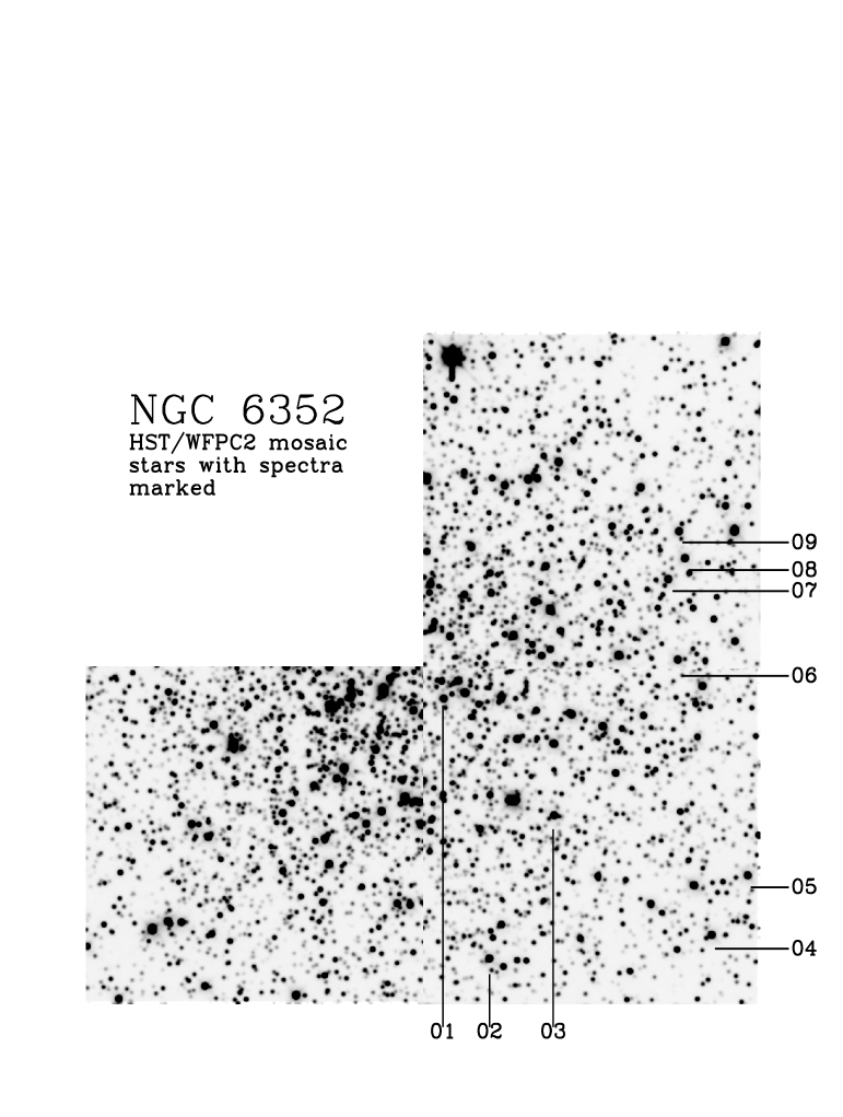
Figure 1: HST/WFPC2 mosaic image of NGC 6352 (the PC image is excluded). The stars with UVES spectra are marked with the corresponding numbers from Table 1. This image is created from the following three HST/WFPC2 datasets: u28q0404t, u28q0405t, and u28q040bt.

Stars for the spectroscopic observations were selected based on their position in the CMD. Only a few stars in NGC 6352 have previously been studied with spectroscopy and hence there was no prior knowledge of cluster membership. Therefore we decided to select only stars on the HB in order to maximize the possibility for them to be members. Selecting HB stars rather then RGB and AGB stars has the further advantage that the stars will have fairly high effective temperatures ($T_{\rm eff}$) which significantly will facilitate the analysis of the stellar spectra. At lower temperatures the amount of molecular lines start to become rather problematic (see e.g. the discussion in Barbuy 2000; Carretta et al. 2001; Cohen et al. 1999).

The HB in NGC 6352 is situated at $V_{\rm 555}\sim 15.2$. Data for the target stars for the spectroscopic programme are listed in Table 1. In Fig. 1 we show a mosaic image based on HST/WFPC2 images with the stars observed in the spectroscopic programme labeled by their corresponding numbers from Table 1. The table also includes a cross-identification with designations used in other major studies of NGC 6352 (Alcaino 1971; Hartwick & Hesser 1972).

3 Spectroscopy

3.1 Observations and data reduction

Observations were carried out in service mode as part of observing programme 69.B-0467 with the UVES spectrograph on Kueyen. We used the red CCD with a standard setting centered at 580.0 nm. With this setting we cover the stellar spectra from 480.0 to 680.0 nm with a gap between 576.0 nm and 583.5 nm. Each star was observed for 4800 s in a single exposure.

The spectra were pipeline calibrated as part of the service mode operation. As our spectra are of moderate S/N (in the red up to 80, but in the blue more like 60) we have visually inspected the reduced and extracted one-dimensional spectra for known foibles and found them to not suffer from any of these problems.

3.2 Radial velocity measurements and cluster membership

Radial velocities were measured from the stellar spectra using the rv suite of programs inside iraf. From the observed radial velocities helio centric velocities and velocities relative to the local standard of rest (LSR) were calculated and are listed in Table 2. We find the cluster to have a mean velocity relative to the LSR of –120.7 km s^-1 with $\sigma=3.7$ km s^-1. All of our program stars have velocities that deviate less then 2$\sigma$ from the mean velocity. Hence they are all members.

The most recent value for $V_{\rm LSR}$ in the catalogue of globular clusters (Harris 1996, catalogue ) is $-116.7$ km s^-1. This is in reasonably good agreement with our new result based on data for nine stars. The Harris (1996) value is based on a weighted average from three studies (Rutledge et al. 1997; Zinn & West 1984; Hesser et al. 1986). Rutledge et al. (1997) found $V_{\rm Helio}=-122.8$ km s^-1 for a sample of 23 stars. Using the following equation

$$V_{\rm LSR}=V_{\rm Helio}+11.0\cos b\cos l+14.0\cos b\sin l+7.5\sin b$$

(Ratnatunga et al. 1989), with $l=341.4$ and $b=-7.2$ for NGC 6352, this corresponds to a $V_{\rm LSR}=-117.9$ km s^-1. We note that Rutledge et al. (1997) estimate their external errors for the measurement of the radial velocities for stars in NGC 6352 to be on the order of 10 km s^-1. More recently, Carrera et al. (2007) find $V_{\rm Helio}=-114$ km s^-1 based on 23 stars, which is equivalent to $V_{\rm LSR}=-109$ km s^-1. No estimate of external errors are given in their study. Their value is more similar to that measured by Hartwick & Hesser (1972), $V_{\rm Helio}=-112.2$ km s^-1, than to ours. There are no stars in common between our study and Carrera et al. (2007).

Hence, it does appear that our estimate of $V_{\rm LSR}$ for NGC 6352 is somewhat high when compared to other estimates available in the literature. However, as we do not have a good estimate of zero-point errors for the various studies and as no doubt different types of stars have been used in the various studies, e.g. we use only HB stars whilst some of the earliest studies clearly will have relied on very cool giants where e.g. motions in the stellar atmospheres might play a role (Carney et al. 2003), and since we have no information on binarity for any of these stars the current value should be regarded as being in good agreement with previous estimates.

Table 2: Measured and derived velocities. The second column gives the radial velocity of the star as measured from the stellar spectrum. The third column the derived helio centric velocity and the fourth the velocity relative to the local standard of rest (LSR). The last line gives the mean helio centric velocity for all the stars and the corresponding standard deviation as well as the mean LSR velocity with its corresponding standard deviation.

Star	$V_{\rm 0bs}$	$V_{\rm Helio}$	$V_{\rm LSR}$
	km s-1	km s-1	km s-1
NGC 6352-01	–154.30	–146.18	–127.36
NGC 6352-02	–147.13	–142.05	–123.24
NGC 6352-03	–141.65	–136.72	–117.90
NGC 6352-04	–140.71	–135.87	–117.06
NGC 6352-05	–144.62	–139.90	–121.09
NGC 6352-06	–137.72	–133.75	–114.94
NGC 6352-07	–143.60	–139.52	–120.71
NGC 6352-08	–144.81	–140.63	–121.82
NGC 6352-09	–148.53	–141.31	–122.50
NGC 6352		–139.5 $\sigma=3.7$	–120.7 $\sigma=3.7$

3.3 Measurement of equivalent widths

Equivalent widths were measured using the splot task in iraf. For each line the local continuum was estimated with the help of synthetic spectra generated using appropriate stellar parameters and a line-list, typical for a K giant, from VALD, see Piskunov et al. (1995), Ryabchikova et al. (1999), and Kupka et al. (1999). The equivalent widths used in the abundance analysis are listed in Table LABEL:eqw.tab.

3

Table 3: Measured equivalent widths used in the abundance analysis. Column one lists the element and the ionizational state for the line, col. 2 the wavelength (in Å), col. 3 the excitation energy of the lower level involved in the transition, col. 4 the oscillator strength (see Sect. 4 for references). Cols. 5 to 13 then lists the measured equivalenth widths in mÅ for each star, as indicated in the header. The stars are identified in Fig. 1 and Table 1).

El	$\lambda$	$\chi_{\rm l}$	$\log gf$	NGC 6352-01	-02	-03	-04	-05	-06	-07	-08	-09
Na i	5682.65	2.10	-0.71	89.6	98.7	119.2	93.1	115.6	89.9	88.6	102.5	92.4
Na i	5688.22	2.10	-0.40	113.5	112.6	128.4	111.6	128.4	110.3	110.2	119.3	116.4
Na i	6154.22	2.10	-1.57	36.3	32.2	43.2	30.9	49.4	31.3	28.8	41.2	30.3
Na i	6160.75	2.10	-1.27	49.8	53.5	70.0	43.7	70.2	44.1	47.6	60.2	56.1
Mg i	5711.09	4.33	-1.87	112.7	115.3	116.9	118.1	116.8	118.3	116.5	118.5	121.7
Al i	6696.03	3.14	-1.63	52.0	45.4	46.8		47.0	45.6	41.0	35.5	48.3
Al i	6698.67	3.14	-1.92	21.3	23.6	31.9	23.8	17.5	24.8	23.5
Si i	5128.03	5.08	-2.60	16.0	18.3	18.9	22.2	15.5				22.0
Si i	5517.53	5.08	-2.38	16.2	15.1	18.0	18.8	22.0	16.4	17.6	17.2	17.9
Si i	5621.60	5.08	-2.50	8.0	10.9	6.3	8.2	7.7	5.6	12.7	6.1
Si i	5645.61	4.92	-2.04	40.4	44.1	41.0	40.8	37.0	40.6	41.6	45.1	44.5
Si i	5665.55	4.93	-1.94	50.7	49.2		46.7	48.9	43.8	51.9	44.8	45.3
Si i	5684.48	4.95	-1.55	66.5	65.7	67.4	57.2	61.1	64.9	65.3	65.8	67.0
Si i	5701.12	4.93	-1.95	45.0	42.9	38.0	42.6	35.9	49.9	44.1	45.0	44.0
Si i	5948.54	5.08	-1.13	94.1	87.1	91.3	92.6	91.7	83.6	90.5	88.6	94.0
Si i	6125.03	5.61	-1.52	30.6	33.7	27.4	33.1	28.8	30.5	31.3	28.5	33.2
Si i	6142.49	5.62	-1.50	34.9	37.7	31.1	29.8	30.4	32.9	33.2	32.4	38.2
Si i	6145.02	5.61	-1.46	33.5	36.4	32.8	31.8	36.1	36.9	35.4	29.9	34.5
Si i	6155.14	5.62	-0.72	76.6	73.5	70.6	70.7	67.4	69.2	75.0	73.2	72.0
Si i	6555.46	5.98	-1.00	48.4	44.5		30.6			31.8	14.2	38.3
Ca i	5260.39	2.52	-1.71	44.6	46.7	39.6	42.1		34.6	36.9	36.4	39.6
Ca i	5512.98	2.93	-0.44	89.5	88.7	86.2	89.2	87.5	87.5	86.7	85.9	91.9
Ca i	5581.97	2.52	-0.55	101.2	102.5	97.6	103.4	102.2	97.9	101.8	96.7	103.9
Ca i	5601.28	2.53	-0.52	124.1	116.0	108.7	109.3	105.3	112.9	105.0	110.0	102.1
Ca i	6161.30	2.52	-1.26	76.4	76.3	65.1	71.6	62.5	74.4	69.3	68.2	75.8
Ca i	6166.44	2.52	-1.14	81.1	83.0	77.6	76.9	75.4	77.0	76.6	73.9	85.5
Ca i	6169.04	2.52	-0.79	101.4	100.6	92.6	98.0	100.0	95.6	96.9	96.5	109.1
Ca i	6169.56	2.52	-0.47	118.9	110.9	113.3	115.0	112.5	111.1	109.3	110.1	120.1
Ca i	6439.08	2.52	0.39	164.5	168.8	160.0	172.4	168.6	168.4	163.4	170.0	164.6
Ca i	6455.61	2.52	-1.29	65.1	70.1	64.9	57.2	62.6	64.0		61.7	60.4
Ca i	6471.67	2.52	-0.68	102.6	105.1	102.4	99.0	94.7	96.9	101.1	94.7	107.1
Ca i	6493.79	2.52	-0.10	139.9
Ca i	6499.65	2.52	-0.81	96.9	96.9	99.0	100.4	94.1	99.5	95.5	96.2	102.9
Ti i	4885.08	1.88	0.41		100.7	92.4	99.1	92.5	101.7	91.9	91.6	106.8
Ti i	4913.62	1.87	0.22	76.0	79.1	76.1	79.5	75.9	76.5	74.3	72.2	79.8
Ti i	4915.23	1.88	-0.96	15.5	21.5	11.2	20.6	16.9	17.0	15.9	11.5
Ti i	4981.73	0.84	0.56	155.4	152.6	141.6	148.2	139.4	150.2	135.3	146.3	154.0
Ti i	4997.09	0.00	-2.06	83.8	84.0	74.6	79.8	73.3	73.8	71.1	72.6	75.2
Ti i	5000.99	1.99	0.02	62.5	55.5	55.5	71.1	51.5	62.2	54.2	55.9	61.8
Ti i	5016.16	0.85	-0.52	103.5	106.1	100.0	106.4	95.2	102.2	101.7	98.8	101.6
Ti i	5020.02	0.83	-0.35	118.0	118.3	116.0	117.9	117.8	116.1	120.0	113.5	116.5
Ti i	5022.87	0.83	-0.38	114.7		107.8	113.2	113.9	104.7	108.2	104.7	110.3
Ti i	5024.85	0.82	-0.55	110.6	107.3	101.8	104.3	104.1	100.7	102.7	96.2	109.8
Ti i	5043.59	0.83	-1.67	45.4	48.9	46.7	58.4	45.4	43.3	45.3	41.6	49.2
Ti i	5062.10	2.16	-0.40		29.1	25.2	23.1	23.9	23.2	25.8	21.7	25.1
Ti i	5071.46	1.46	-1.00	43.3	50.4	44.2		46.6	47.5	43.4		47.0
Ti i	5087.06	1.43	-0.78		57.7	54.8	63.9	47.8	54.4		48.3	59.7
Ti i	5113.45	1.44	-0.73	54.3	55.4	50.5	56.2	49.4	49.2	46.7	46.0	55.0
Ti i	5145.46	1.46	-0.51	61.0	63.6	60.7	66.6	64.0	60.7	60.8	57.8	67.0
Ti i	5147.47	0.00	-1.95	85.0	88.1	78.6	84.1	79.0	81.4	78.4	73.1	87.7
Ti i	5201.08	2.09	-0.69	22.6	18.7	23.7	25.4	27.3	21.0	22.7	19.0	26.2
Ti i	5210.38	0.04	-0.82	138.7	148.5	140.5	145.2	131.5	137.5	136.8	134.0	142.5
Ti i	5219.70	0.02	-2.24	71.7	71.5	70.2	71.5	68.3	65.3	66.1	61.7	71.5
Ti i	5223.62	2.09	-0.50	32.3	28.6	34.4	29.6	33.9	27.8	30.1	26.8	30.0
Ti i	5426.26	0.02	-2.95	28.6	27.9	29.9	34.2	24.9	31.6	27.4	23.7	28.4
Ti i	5471.20	1.44	-1.40	21.8	24.8	26.0	21.8	15.3	24.6	23.5	20.7	21.1
Ti i	5474.23	1.46	-1.23	23.0	32.2	26.7	36.8	31.4	26.5	38.1	30.2	34.4
Ti i	5490.15	1.46	-0.88	53.1	54.9	47.8	55.0	48.8	46.6	49.0	44.2	50.2
Ti i	5662.15	2.31	-0.05	40.9	45.3	36.5	45.9	43.1	42.3	42.3	34.0	47.6
Ti i	5679.91	2.47	-0.41	12.7	11.5	9.9	11.2		7.0	11.6	4.4	13.3
Ti i	5689.46	2.29	-0.36	20.4	22.2	15.7	25.4	20.2	20.3	20.4	16.9	22.6
Ti i	5702.65	2.29	-0.59	13.0	20.2	23.7	22.8	15.1		13.3	19.6	17.6
Ti i	5716.44	2.29	-0.72	11.9	15.6	9.1	12.3	14.5	14.3	11.4	10.9	13.3
Ti i	5866.46	1.07	-0.78	87.6	90.5	84.5	83.7	83.0	82.4	85.0		89.3
Ti i	5880.26	1.05	-1.70			25.2
Ti i	5918.53	1.06	-1.46		36.5	35.9	38.0	35.2	30.5	33.4		39.1
Ti i	5922.11	1.04	-1.41	58.7	54.1	50.3	55.9		46.4	46.5	41.3	58.7
Ti i	5937.80	1.06	-1.84	22.1	23.6	16.6	29.9	20.1	19.0	21.0	15.4	22.9
Ti i	5953.17	1.89	-0.27	73.4	66.1	63.4	71.0	60.8	62.5	66.1	59.4	66.7
Ti i	6126.22	1.07	-1.37	53.7	57.3	47.1	58.9	44.4	54.1	47.3	43.5	59.6
Ti i	6258.11	1.44	-0.30	87.4	85.6	80.2			76.3	80.2	75.3	93.3
Ti i	6261.11	1.43	-0.42	74.1	77.4	79.3	85.0	71.3	85.0	81.3	72.9	81.1
Ti i	6743.13	0.89	-1.63	44.8	36.5	42.3		40.9	44.8	44.9	34.8	53.9
Ti ii	4849.18	1.13	-3.00	83.7	83.1	78.1	77.5	83.0	80.7	81.7	80.3	83.1
Ti ii	4865.61	1.11	-2.79	87.3	88.6	83.2	75.8	81.6	86.3	74.6	85.8	84.4
Ti ii	4874.01	3.09	-0.80	63.0	60.9	56.0	57.8	60.2	61.7	69.5	58.2	58.1
Ti ii	4911.19	3.12	-0.61	73.4	75.8	86.1	76.5	67.3	76.5	77.5	72.8	80.9
Ti ii	5005.15	1.56	-2.72	58.5	50.6	52.6	52.0	51.6	53.2	52.2	53.2	53.6
Ti ii	5013.33	3.09	-1.91				80.3	70.4	80.4	80.3	77.5	81.0
Ti ii	5013.67	1.58	-2.19	88.8	84.1	83.6	97.4	88.0	89.8	90.4	91.5	98.4
Ti ii	5154.07	1.56	-1.75	108.6	100.3		110.2	92.3	113.4	99.7	108.1	104.3
Ti ii	5185.91	1.89	-1.49	98.1	98.7	101.4	102.2	104.5	96.7	99.9	103.8	103.8
Ti ii	5336.77	1.58	-1.59	110.1	106.3	111.2	110.1	109.9	106.7	108.5	109.6	108.2
Ti ii	5381.01	1.56	-1.92	101.6	98.5	105.5	98.2	99.5	100.6	103.8	97.7	94.3
Ti ii	5418.75	1.58	-2.00	88.2	84.1	86.8	86.8	82.0	88.0	90.1	88.8	86.0
Ti ii	6491.56	2.06	-1.89	76.3	69.4	63.8	69.2	66.9	69.8	72.0	68.3	64.9
Ti ii	6559.58	2.04	-2.13	58.5	54.7	55.7	52.3	53.8	52.5	53.5	51.1	51.4
Ti ii	6606.94	2.06	-2.76	23.1	29.8	26.4	25.7		22.5	25.1		32.9
Ti ii	6680.13	3.09	-1.78	19.8	19.4	18.8	19.2	12.0	14.3	18.9
Cr i	5238.96	2.71	-1.43	16.1			20.4	16.3	14.9		12.5
Cr i	5296.69	0.98	-1.41	117.0	110.7	110.3	119.0	112.1	112.4	114.9	108.9	113.9
Cr i	5300.74	0.98	-2.12	79.1	83.3	79.2	85.2	75.3	74.9	72.3	71.1	84.3
Cr i	5304.18	3.46	-0.78	15.5	9.3		7.7		8.8	9.0	11.9	11.9
Cr i	5318.77	3.44	-0.77	13.6	16.4	11.8	13.8	10.4	13.4	17.1		19.4
Cr i	5348.31	1.00	-1.29	123.7	116.7	121.0	119.9	113.9	117.6	114.5	115.9	119.6
Cr i	6330.09	0.94	-2.90	37.6	42.0	36.4	38.5	34.9	37.6	28.5	33.8	41.9
Cr i	6630.03	1.03	-3.60	17.0	13.4	10.6	11.3	11.7		15.0	6.7	12.9
Cr ii	4848.25	3.86	-1.14	64.2		79.7		71.1	57.0	67.3	68.1	69.7
Cr ii	5237.32	4.07	-1.18	57.8	57.4	58.2	58.3	55.0		58.5	55.2	53.5
Cr ii	5305.85	3.82	-2.06	30.4	26.3	27.2	24.0	25.8	29.2		31.1	30.7
Cr ii	5310.68	4.07	-2.24	13.5		12.8		14.9		18.9	11.0	12.6
Cr ii	5313.56	4.07	-1.55	43.0	33.7	34.5		39.5	33.7	39.2		38.6
Cr ii	5502.06	4.16	-1.97	20.7	20.7	24.7	20.4	22.2	23.7	22.5		13.1
Fe i	4802.88	3.64	-1.51	49.8	64.0	57.2	53.8	58.5			55.5	58.3
Fe i	4834.50	2.42	-3.41	54.2	55.9	56.4	57.3	48.0	54.8	51.0	54.8	60.1
Fe i	4839.54	3.27	-1.82	77.0	70.4	77.7	79.7	74.9	74.7		79.2	83.8
Fe i	4848.88	2.27	-3.14	61.5	63.6	55.2	69.0	58.8	54.4	54.5	54.4	56.6
Fe i	4849.66	3.57	-2.68									13.6
Fe i	4874.35	3.07	-3.03	27.8	38.9	34.2	26.4	28.9	24.4	36.2	23.5	27.9
Fe i	4882.14	3.42	-1.64	75.2	88.5	81.6	89.8	81.9	83.7	89.0	78.5	93.4
Fe i	4892.85	4.21	-1.29	55.3	57.8	52.4	57.2	54.8	51.0	56.7	46.9	56.6
Fe i	4896.43	3.88	-2.05	39.7	40.0	34.2	43.5	33.8	35.8	37.7	34.3	41.0
Fe i	4907.73	3.43	-1.84	67.1	67.0	65.1	64.6	67.7	63.9	64.5	65.9	71.6
Fe i	4911.77	3.92	-1.79	51.5	56.1		62.1	49.3	48.1	51.9	39.5	56.1
Fe i	4917.23	4.19	-1.18	66.8	68.8	64.8	65.8	57.9	60.7	66.1	66.1	66.6
Fe i	4927.41	3.57	-2.07	61.0	59.4	59.3	61.3	53.1	57.6	55.5	46.0	50.7
Fe i	4946.38	3.37	-1.17	103.6	105.6	105.6	103.6	102.2	106.9	105.2	100.6	105.9
Fe i	4950.10	3.41	-1.67	82.4	87.5	80.1		87.0	81.7	74.2	83.6	85.1
Fe i	4961.92	3.63	-2.19	32.8	31.3	33.4	32.3	35.4	34.1	28.9	30.1	34.7
Fe i	4962.57	4.18	-1.18	57.7	51.9	54.1	55.3	52.3	52.9	52.9	49.6	54.4
Fe i	4969.91	4.21	-0.71	78.7	78.1	76.9	79.5	72.8	80.2	80.2	73.6	83.1
Fe i	4979.58	3.64	-2.58	24.2	28.7	21.2	26.3	19.6	22.3	19.9	20.8	24.2
Fe i	4985.25	3.92	-0.56	95.2	94.4	83.3	92.9	91.5	95.9	98.7	93.5	97.0
Fe i	4985.54	2.86	-1.33	116.6	119.2	111.7	115.0	105.6	111.9	111.2	112.4	116.7
Fe i	4986.22	4.21	-1.39	49.1	49.2	52.1	55.6	43.3	48.3	47.5	40.6	50.2
Fe i	4999.11	4.18	-1.74	37.6	31.6	48.2	40.3	25.0	35.3	28.8		34.9
Fe i	5001.86	3.88	0.01	118.6	114.0	119.1	115.0	113.6	116.3	115.9	118.0	113.5
Fe i	5004.04	4.20	-1.40	47.8	45.2	48.6	57.8	44.0	44.4	48.7	45.5	51.7
Fe i	5012.69	4.28	-1.79	36.6	39.0	35.2	37.9	32.2	36.2	32.3	32.0	39.7
Fe i	5014.94	3.94	-0.30	114.5	110.9	112.2	118.2	116.2	111.3	111.5	111.8	118.1
Fe i	5016.47	4.25	-1.69	18.7		31.4	32.4	36.3	34.2	32.7	26.0	31.5
Fe i	5028.12	3.57	-1.12	95.8	94.6	91.2	95.8	90.2	91.1	91.5	84.7	92.6
Fe i	5031.91	4.37	-1.67	28.9	26.2	27.9	35.4	21.1	19.3	21.1	20.3	27.1
Fe i	5044.21	2.85	-2.06	90.2	91.0	95.1	90.7	92.2	90.1	90.7	88.4	93.2
Fe i	5054.64	3.64	-1.92	40.5	42.5	35.5	45.5	37.0	38.4	43.3	32.8	40.6
Fe i	5056.84	4.26	-1.96	30.8	35.1	25.1	29.2	21.1	24.5	29.6	21.4	35.7
Fe i	5058.49	3.64	-2.83	13.9	16.5	13.3	13.5	8.1	13.6	8.7	6.3	12.0
Fe i	5067.16	4.22	-0.97	72.0	75.5	70.3	70.0	67.0	69.5	68.1	68.6	71.9
Fe i	5083.33	0.95	-2.96	146.9	152.7	141.0	147.2	146.8	144.9	142.1	138.1
Fe i	5088.15	4.15	-1.68	36.0	35.0	25.1	35.5	32.5	32.9	32.5	29.0	37.6
Fe i	5090.77	4.26	-0.40	81.9	91.8	83.5	90.7	85.8	90.5	92.4	86.5	88.9
Fe i	5104.44	4.28	-1.59	37.1	39.2	35.7	36.3	37.9	36.4	34.2	35.1	42.3
Fe i	5109.66	4.30	-0.98	67.7	68.8	71.1		73.7	66.9	64.2	71.7	63.0
Fe i	5115.77	3.57	-2.74	28.3	30.7	14.6	26.9	18.4	22.3	26.2	16.3	25.3
Fe i	5127.37	0.91	-3.31	130.2	129.4	129.7	123.7	132.1	133.3	130.7	129.6	136.9
Fe i	5127.67	0.05	-6.12	55.7	56.9	50.3	62.0	55.2	51.6	48.7	49.5	55.9
Fe i	5141.75	2.42	-2.24	103.5	104.2	101.6	103.9	105.5	101.9	102.2	99.1	106.9
Fe i	5143.72	2.19	-3.79	44.4	38.3	37.1	44.7	33.2	35.2	35.3	32.7	43.0
Fe i	5145.09	2.19	-2.88	79.3	75.5	69.9	69.2	69.9	71.7	71.7	70.0	76.4
Fe i	5159.05	4.28	-0.82	64.7	63.5	68.3	67.5	59.1	61.8	65.5	64.6	65.8
Fe i	5187.91	4.14	-1.37	63.8	57.4	58.0	55.5	55.9	55.5	57.0	55.2	54.5
Fe i	5197.93	4.30	-1.64	34.9	35.1	32.5	41.8	40.4	28.8	34.8	30.4	32.1
Fe i	5198.71	2.22	-2.14	123.9	125.5	119.1	118.4	120.6	113.6	120.1	112.5	121.0
Fe i	5209.88	3.23	-3.26	37.4	23.7	27.0	17.8	15.8	14.0
Fe i	5217.38	3.21	-1.16	117.0	117.2	109.8	111.6	111.0	113.6	110.3	108.8	111.4
Fe i	5223.18	3.63	-1.78	30.2	39.0	29.7		32.9	28.3	37.7	29.8	31.8
Fe i	5242.49	3.63	-0.97		92.3	91.7	92.3	93.4	90.1	93.6	90.2	85.6
Fe i	5249.10	4.47	-1.48	35.3	38.4	24.2	39.8	30.8	36.6	34.3	30.7	36.8
Fe i	5253.03	2.27	-3.84	30.5	26.7	27.9	32.2	27.9	27.8	32.7	23.9	30.1
Fe i	5262.88	3.25	-2.66	25.5		25.9	29.4	20.0	31.3	28.4	21.1	21.9
Fe i	5263.86	3.57	-2.14	71.4	66.7	66.1	67.2	49.5		52.7	54.7	66.2
Fe i	5267.26	4.37	-1.77	26.3	23.8	23.7	30.3	19.8	20.4	31.4	20.0	19.2
Fe i	5285.12	4.43	-1.64		33.4	26.8	23.5	21.9	23.6	21.1	20.1	25.0
Fe i	5288.53	3.68	-1.51	65.2	62.3	69.3	65.6	62.9	64.7	66.3	62.6	65.8
Fe i	5293.95	4.14	-1.87	32.3	28.4	26.1	26.1	28.7	26.1	27.5	25.1	28.0
Fe i	5294.54	3.64	-2.76	15.6	16.5	10.5	16.0	18.1	13.9	12.1	12.4	11.6
Fe i	5295.31	4.41	-1.59	28.3	28.2	23.4	25.8	23.4	26.5	19.9	21.3	23.9
Fe i	5307.36	1.61	-2.99	121.1	119.3	111.6	123.7	119.7	117.8	117.6	112.9	122.6
Fe i	5321.10	4.43	-0.95	39.2	41.3	38.8	39.7	37.8	39.5	39.0	38.9	41.7
Fe i	5322.04	2.28	-2.80	84.0	83.5	81.0	80.7	81.1	77.9	78.7	76.4	82.8
Fe i	5364.87	4.44	0.23	107.2	110.8	108.2	106.3	107.5	109.1	111.7	108.2	109.9
Fe i	5365.39	3.57	-1.02	86.0	92.4	87.6	82.4	91.2	83.3	87.9	84.5	85.3
Fe i	5367.46	4.41	0.44	113.1	121.8	115.6	114.3	119.4	109.0	116.5	112.9	121.2
Fe i	5373.69	4.47	-0.76	62.2	59.0	60.5	59.8	59.3	56.1	63.0	57.3	58.9
Fe i	5379.57	3.69	-1.51	65.3	69.3	69.8	64.4	65.1	64.2	64.9	57.6	66.1
Fe i	5383.36	4.31	0.64	127.8	134.7	130.6	128.6	130.4	131.6	133.0	124.0	130.9
Fe i	5386.33	4.15	-1.67	34.5	35.8	25.0	28.4	24.0	29.0	29.5	23.8	29.1
Fe i	5389.47	4.41	-0.41	86.2	86.7	78.7	78.1	83.8	82.0	81.8	77.6	81.5
Fe i	5395.21	4.44	-2.07	15.6	16.8	18.6	26.4	16.0	12.2		15.2	23.6
Fe i	5398.27	4.44	-0.63	73.7	54.1	69.1	68.8	66.3	67.0	73.2		75.7
Fe i	5410.90	4.47	0.40	115.2	108.0	112.8	103.3	107.3	105.3	109.2	105.0	106.6
Fe i	5412.78	4.43	-1.89	22.5	17.2		18.7		11.6		16.3	19.6
Fe i	5436.59	2.27	-2.96	67.3	69.8			64.2	66.8	67.7	65.1	72.3
Fe i	5441.34	4.31	-1.63	27.8	33.3	27.1	29.6	28.8	29.5	28.2	25.9	30.7
Fe i	5445.04	4.38	-0.02	106.2	103.2	104.9	102.0	103.9	107.2	108.4	101.7	106.9
Fe i	5452.08	3.64	-2.86	25.1	28.1				27.6	12.1	21.5	20.7
Fe i	5460.87	3.07	-3.58	9.2		15.6	12.4	8.4	19.4	9.2	8.3	10.2
Fe i	5461.55	4.44	-1.80	29.7		23.7	26.0	25.1	22.4	22.1	23.3	28.2
Fe i	5463.27	4.43	0.11	103.8	100.0	104.4		97.6	95.6	96.9	96.5	98.8
Fe i	5464.28	4.14	-1.40	38.8	38.6	32.3	39.2	42.7	35.8	33.5	35.5	43.8
Fe i	5466.99	3.57	-2.23	35.3	33.1	30.2	37.6	38.7	33.4	37.1	35.5	36.6
Fe i	5470.09	4.44	-1.81	21.4	20.1	17.0	19.3		24.6	21.2	21.3	23.7
Fe i	5501.46	0.95	-3.05	158.5		152.8	162.2	150.3		153.6	146.0	158.4
Fe i	5522.44	4.20	-1.45	42.6	41.6	41.9	41.4	36.7	39.1	29.7	39.6	41.0
Fe i	5539.28	3.64	-2.66	22.8	15.0	19.4	24.7	18.8	20.0	23.6	16.2
Fe i	5543.93	4.21	-1.14	58.9	57.7	59.3	59.2	56.5	54.7	60.5	56.4	48.8
Fe i	5546.50	4.37	-1.21	50.6	53.2	47.3	52.1	51.1	52.5	51.6	48.4	51.5
Fe i	5554.89	4.54	-0.44	86.4	84.1	80.3	83.6	84.0	82.1	84.1	84.9	88.1
Fe i	5560.20	4.43	-1.09	51.0	50.3	47.3	45.1	53.3	43.5	45.6	44.9	49.5
Fe i	5576.10	3.43	-0.90	118.2	119.3	112.0	112.7	94.9	110.0	117.3	107.5	116.6
Fe i	5587.57	4.14	-1.85	34.9	37.4	33.7	33.9	31.2	30.8	33.8	32.4	38.3
Fe i	5618.63	4.20	-1.28	50.5	43.8	47.5	44.5	54.5		51.2	49.6
Fe i	5619.59	4.38	-1.60	34.0	35.7	31.1	30.0	31.9	26.9	31.0	30.1	32.5
Fe i	5624.02	4.38	-1.48	42.0	34.2	40.0	45.1	49.5	47.0	49.6		50.3
Fe i	5633.94	4.99	-0.27	61.1	59.1	55.8	57.8	55.6	57.6	58.0	54.0	60.0
Fe i	5635.83	4.25	-1.79	25.4	31.5	29.9	30.2	28.0	30.5	22.7	26.9	33.2
Fe i	5638.26	4.22	-0.87	71.3	74.5	71.7	75.1	72.6	74.1	74.6	73.2	76.2
Fe i	5649.98	5.09	-0.92	28.2	30.2	29.4	28.0	20.1	24.0	26.6	29.3	31.1
Fe i	5650.70	5.08	-0.96	26.1		27.2	31.7	30.7	26.6	27.3	26.3	32.8
Fe i	5651.47	4.47	-1.90	14.7	20.8		18.9	17.2	16.0	15.1	12.7	15.3
Fe i	5652.31	4.26	-1.85	27.0	26.0	20.1	25.2	23.0	24.1	21.4	26.2	23.8
Fe i	5653.86	4.38	-1.64	34.3	36.3	32.6	38.3	28.4	35.7	32.0	32.5	39.3
Fe i	5661.34	4.28	-2.02	26.5	26.9	22.0	24.5	26.8	21.7	22.9	21.7	26.7
Fe i	5662.51	4.17	-0.57	92.8	93.0	90.1	89.1	89.4	95.4	87.2	93.4	99.2
Fe i	5667.51	4.17	-1.58	50.6	55.0	50.8	55.6	41.3	53.7	55.6	45.0	51.8
Fe i	5679.02	4.65	-0.82	40.0	52.4	46.8		50.7	47.9	53.4	46.4	52.6
Fe i	5680.24	4.18	-2.58	14.3
Fe i	5691.49	4.30	-1.52	47.4	44.3	36.6	33.2	32.2	35.0	38.1	34.0	37.1
Fe i	5701.54	2.56	-2.12	105.7	102.0	97.4	99.5	104.1	103.5	98.2	100.9	109.1
Fe i	5705.46	4.30	-1.50	38.3	36.2	31.6	36.7	31.7	38.2	33.5	34.1	38.0
Fe i	5717.83	4.28	-1.13	61.0	65.0	57.6	66.4	70.1	64.3	62.6	65.5	67.3
Fe i	5731.76	4.25	-1.20	54.1	55.4	54.3	53.6	60.0	55.7	56.5	57.6	57.8
Fe i	5741.84	4.25	-1.85	26.6	28.4	23.6	30.3	22.9	22.6	26.4	25.4
Fe i	5752.02	4.54	-0.66	48.8	49.0	46.8	49.3	51.2	48.8	49.7	48.1	50.5
Fe i	5753.13	4.26	-0.69	79.4	77.1	76.9	74.6	77.9	79.2	80.3	77.3	82.5
Fe i	5852.21	4.54	-1.23	40.6	44.0	39.1	39.8	38.9	36.5	42.2		36.4
Fe i	5853.14	1.48	-5.28	20.5	17.9	15.6	20.4	19.4	15.6	2.6	18.2	16.6
Fe i	5855.08	4.61	-1.48	21.8	18.9	15.8	20.1		16.1	18.4	14.7	19.4
Fe i	5856.08	4.29	-1.33	31.9	29.9	30.2	31.6	23.6	28.5	30.6	24.8	31.7
Fe i	5859.57	4.54	-0.30	71.3	70.3	70.8	68.7	67.6	66.0	68.2	66.8	71.2
Fe i	5905.67	4.65	-0.73	50.5	50.5	45.3	46.3	41.5	49.1	40.5	44.8	51.6
Fe i	5927.78	4.65	-1.09	46.2	37.0	38.5	40.5	38.4	37.1	37.9	27.8	43.0
Fe i	5929.67	4.54	-1.41	38.4	36.1	31.8	32.1	33.9	32.9	32.6	26.2	39.3
Fe i	5930.17	4.65	-0.23	81.3	81.7	80.8	82.9	80.4	82.3	79.0	86.3	84.4
Fe i	5934.65	3.92	-1.17	76.4	75.7	74.3	81.1	75.3	79.6	76.5	73.9	79.7
Fe i	5956.71	0.86	-4.61	88.8	88.7	82.3	87.9	80.6	83.0		79.9	81.7
Fe i	5984.81	4.73	0.17	79.1	75.2	79.2	74.7	78.1	72.4	77.6	76.7	81.8
Fe i	6003.01	3.88	-1.12	80.8	87.0	81.7	83.5	82.3	84.6	82.3	82.4	86.7
Fe i	6012.20	2.22	-4.20	36.4	37.0	28.8	30.2	29.5	34.6	36.2	29.7	31.9
Fe i	6024.05	4.54	-0.12	95.6	93.7	101.2	97.6	91.4	93.5	99.4	94.4	97.5
Fe i	6027.05	4.07	-1.09	66.6	68.3	63.5	62.7	65.4	62.0	69.4	61.1	68.2
Fe i	6056.00	4.73	-0.46	65.7	64.9	61.5	61.7	58.4	60.4	61.4	62.4	65.7
Fe i	6065.48	2.61	-1.53	136.8	135.7	135.2	131.2	141.6	128.3	125.9	124.8	147.1
Fe i	6079.00	4.65	-1.12	33.2	41.9	36.1	39.0	30.0	33.7	42.3	40.7	38.9
Fe i	6082.72	2.22	-3.57	55.3		49.5	50.9	51.5	47.3	51.6	50.8	54.0
Fe i	6085.26	2.75	-2.71	66.4	70.8	64.4	69.2	61.7	65.2	64.7	55.0	69.6
Fe i	6093.64	4.60	-1.40	21.8	27.9	24.3	24.5	23.6	22.2	27.0	21.8	28.1
Fe i	6094.37	4.65	-1.84	16.6	17.3	14.5	14.9	12.2	16.9	16.3	29.0	21.5
Fe i	6096.66	3.98	-1.83	37.8	37.6	33.8	38.2	40.1		36.2	26.3	36.6
Fe i	6120.24	0.91	-5.95	9.8	15.6	9.5	14.4		11.1	8.6	7.9	17.9
Fe i	6127.90	4.14	-1.40	50.4	52.6	46.5	49.1	47.9	52.5	47.6	45.2	55.6
Fe i	6137.69	2.58	-1.40	149.9	154.0		159.8	150.4	152.4	149.3	149.5	141.8
Fe i	6151.61	2.17	-3.27	70.1	70.5	70.4	68.0	63.8	70.8	68.3	64.0	71.1
Fe i	6157.72	4.07	-1.16	70.7	66.8	67.0	59.3	65.6	66.3	67.5	62.5	68.7
Fe i	6159.37	4.60	-1.97	12.7	15.8	11.2	15.3	8.2	6.7	14.7	9.4	10.3
Fe i	6165.36	4.14	-1.47	44.0	45.1	44.4	45.2	38.3	43.4	46.6	41.3	46.3
Fe i	6173.34	2.22	-2.88	97.4	93.7	84.6	89.9	91.7	86.6	86.9	86.5	93.3
Fe i	6180.20	2.72	-2.59	77.0	71.4	68.9	73.0	71.4	72.2	70.5	66.9	76.5
Fe i	6187.99	3.94	-1.62	51.8	50.3	44.9	53.6	46.7	43.7	47.2	46.7	51.3
Fe i	6200.31	2.60	-2.44	94.2	87.4	85.3	83.0	88.2	85.6	88.0	82.2	89.6
Fe i	6213.43	2.22	-2.48	91.5	108.1	102.1	105.1	101.7	99.9	102.0	102.6	108.3
Fe i	6219.28	2.19	-2.42	118.5	116.7	101.1	112.0	110.3	115.1	111.7	110.0	119.8
Fe i	6226.73	3.88	-2.12	26.7	26.8	22.2	25.2	23.6	27.7	25.4	19.2	29.2
Fe i	6229.22	2.84	-2.87	50.3	49.1	49.2	49.6	52.6	49.7	50.1	46.2	49.9
Fe i	6232.64	3.65	-0.96	90.5	87.0	86.3	85.6	87.7	84.7	89.4	82.2	89.8
Fe i	6246.31	3.60	-0.88	112.9	111.2	112.0	112.7	103.5	112.3	112.5	106.6	118.8
Fe i	6252.55	2.40	-1.69	144.3	142.5	143.7	138.1	138.8	138.5	157.1	134.0	152.4
Fe i	6265.14	2.18	-2.55	110.7	113.3	114.0	113.4	114.3	108.9	111.5	115.5	114.9
Fe i	6270.22	2.85	-2.61	72.3	64.8	68.0	60.4	59.6	62.6	66.3	60.4	69.0
Fe i	6297.79	2.22	-2.73	99.5	102.9	96.1		100.3		97.1	97.4	105.5
Fe i	6302.49	3.68	-0.91	98.7	109.6	84.2	77.3		86.4		94.6	64.5
Fe i	6311.50	2.83	-3.23	40.3	47.1	38.3		40.2	44.3	38.9	40.1	37.0
Fe i	6322.68	2.58	-2.43	100.3	72.7	89.4	95.3	89.2	97.4	98.6	96.0	98.7
Fe i	6330.84	4.73	-1.74	33.6	24.3	24.4	22.8	22.8	23.8	25.3	24.0	25.8
Fe i	6335.33	2.19	-2.18	126.2	123.2	115.5	118.6	113.3	119.0	119.3	116.9	122.4
Fe i	6336.82	3.68	-1.05	101.7	105.2	99.6	101.6	97.6	97.2	102.6	99.4	101.8
Fe i	6344.14	2.43	-2.92	83.9	79.6	72.6	76.7	72.9	73.6	79.7	70.5	81.0
Fe i	6355.02	2.84	-2.29	93.1	97.5	95.6			88.3	87.8		92.2
Fe i	6380.75	4.19	-1.38	57.6	55.1	52.2	51.8	51.6	56.2	57.4	75.6	60.1
Fe i	6392.53	2.27	-4.03	23.7	32.4	21.3	29.4	28.0	28.4	26.3	28.4	25.0
Fe i	6393.60	2.43	-1.58	148.0	147.2	152.6	143.0	156.9	140.4	140.0	146.5	166.0
Fe i	6411.64	3.65	-0.72	121.3	120.7	115.3	112.7	116.3	117.6	120.9	112.6	118.7
Fe i	6421.35	2.27	-2.03	144.1	141.5		137.3	135.6	141.5	141.1	139.3	145.1
Fe i	6430.84	2.17	-2.01	145.4	142.2	138.0	139.9	139.7	135.0	138.9	135.2	147.1
Fe i	6475.62	2.55	-2.94	75.0	77.3	72.0	76.1	72.2	71.8	73.1	68.6	75.4
Fe i	6481.87	2.27	-2.96	86.8	80.7	88.5	80.7	82.1	86.2	78.5	81.3	87.8
Fe i	6498.94	0.96	-4.70	95.4	90.4	86.1	95.1	87.4	91.7	82.7	75.2	100.4
Fe i	6533.92	4.55	-1.46	36.3		29.2	32.4	23.0	30.9	29.8	35.8
Fe i	6546.23	2.75	-1.54	127.7	127.8	124.0	115.4	118.6	118.0	120.0	113.6	125.5
Fe i	6569.21	4.73	-0.42	72.9	73.4		77.2	76.1	69.6	60.6	70.1	74.7
Fe i	6574.22	0.99	-5.02	60.7	62.5	57.2	58.2	53.7	53.7	54.6	49.5	60.0
Fe i	6575.01	2.58	-2.71	86.0	81.7	85.5	84.7	85.0	83.2	81.9	82.0	86.6
Fe i	6592.91	2.73	-1.47	136.1		138.5	134.3	129.6	130.8	128.0	127.1	134.5
Fe i	6593.87	2.43	-2.42	111.3	107.7	109.2	104.1	102.5	115.1	112.1	106.9	109.3
Fe i	6597.56	4.79	-1.07	36.1	36.3	38.7	33.2	33.8	36.8	37.4	32.1	40.6
Fe i	6627.56	4.55	-1.58	18.2	23.2	28.1	26.9	25.2	19.7	25.2	23.8	20.7
Fe i	6646.93	2.60	-3.99	14.2	17.2	13.9	18.0	17.4	20.3	18.0	19.5	21.9
Fe i	6677.99	2.68	-1.42	144.4	148.9	145.4	129.0	143.1	142.6	139.8	139.0	148.1
Fe i	6703.56	2.75	-3.06	43.7	49.2	50.0	50.3	46.1	48.0	45.7	47.3	51.1
Fe i	6710.31	1.48	-4.88	32.8	33.7	34.0		29.4	33.4	30.3	29.4	31.8
Fe i	6713.74	4.79	-1.50	16.8	19.5	16.2	19.7		17.4	13.2	13.5	12.2
Fe i	6715.38	4.60	-1.64	21.0	24.9	30.3	22.0	23.9	25.0	27.8	18.5	27.7
Fe i	6725.35	4.10	-2.30	16.1	15.1		17.0	15.2	11.0	17.6	14.4	20.0
Fe i	6726.66	4.60	-1.00	37.7	39.2	33.3	30.5	38.4	39.2		33.3	43.5
Fe i	6739.52	1.55	-4.95	22.9	26.1	16.8	24.5	17.8	25.7	24.4	16.6	29.5
Fe i	6750.15	2.42	-2.62	97.6	98.7	96.5	69.4	93.5	95.2	95.6	91.3	98.3
Fe i	6786.86	4.19	-2.07	25.1	24.9	19.7	14.5	23.4	26.2	25.6	25.6	28.9
Fe ii	4993.35	2.81	-3.52	49.7	51.3	51.3	43.4	53.8	48.0	49.1	49.1	50.1
Fe ii	5234.63	3.22	-2.28	95.8	95.7	101.4	96.3	97.0	97.8	99.3	97.7	91.2
Fe ii	6416.93	3.89	-2.88	32.7	37.9	37.1		39.1	35.9	41.0	36.0	45.1
Fe ii	5991.37	3.15	-3.65			36.1						36.1
Fe ii	6084.11	3.19	-3.88	22.5	22.7		24.1	27.8	24.9	26.3	24.2
Fe ii	6149.25	3.88	-2.84	37.1		39.8	37.4	34.7	36.0	38.3	35.8	40.3
Fe ii	6247.55	3.89	-2.43	59.5	54.3	62.6	52.8	58.9	59.3	56.4	60.6	57.1
Fe ii	6369.46	2.89	-4.23		27.0	25.5	22.6	24.3	23.2	25.7	22.3	23.3
Fe ii	6432.68	2.89	-3.69	52.3	47.4	40.3		50.7	48.0	44.8	47.7	48.7
Fe ii	6456.38	3.90	-2.19	63.4	66.5	66.4	65.8	72.4	66.5	63.1	75.2	61.1
Fe ii	6516.08	2.89	-3.43	61.7	66.3	65.5	62.9	63.8	67.4	66.5
Fe ii	4923.92	2.89	-1.50	194.7	177.7	172.3	207.2	205.7	198.1	202.5	208.3	191.4
Fe ii	5132.66	2.80	-4.09	29.1		27.1	23.7	37.4		34.6		26.3
Fe ii	5197.57	3.23	-2.35	95.8	98.7	93.8	97.3	100.7	93.2	97.2	95.2	96.8
Fe ii	5264.81	3.23	-3.13	57.9			53.3	53.9	59.4	58.8	60.0	57.5
Fe ii	5284.10	2.89	-3.20	73.8	81.0	80.7	79.3	83.2	76.2	77.5	76.4	78.3
Fe ii	5325.55	3.22	-3.32	52.4	52.8	49.5	47.8	50.9	49.0	55.3	54.8	53.4
Fe ii	5414.07	3.22	-3.64	31.7	32.0	35.5	34.2	34.2	30.4	38.7	33.7	35.2
Fe ii	5425.25	3.19	-3.39	47.2	46.5	44.0	42.5	44.6	51.9	52.5	52.1	48.6
Fe ii	5534.83	3.25	-2.86	60.7	62.7	73.2	67.9	73.2	63.8	60.9	69.4	68.9
Ni i	4866.26	3.53	-0.21	81.8	92.2	86.0	84.8	85.0	85.1	83.9	86.2	87.3
Ni i	5082.33	3.65	-0.54	67.9	73.3	63.6	74.7	67.9	68.9	70.9	59.1	72.5
Ni i	5094.40	3.83	-1.11	26.4	27.5	27.7	30.4	28.8	19.3	29.1	27.0	33.6
Ni i	5587.85	1.93	-2.44	79.8	82.7	77.8	76.4	77.5	77.7	81.7	72.2	81.8
Ni i	5593.73	3.89	-0.78	43.9	42.0	44.1	41.0	39.8	42.2	43.5	33.7	42.5
Ni i	5748.34	1.67	-3.24	54.3	49.6	51.9	50.1	52.1	48.7	91.4	46.0	53.0
Ni i	6108.10	1.67	-2.43	89.4	96.3	96.0	89.1	91.5	91.2	13.4	87.7	96.1
Ni i	6111.06	4.08	-0.82	31.9	31.1	32.3	34.6	35.1	32.9	17.6	28.8	30.9
Ni i	6130.13	4.26	-0.88	16.3	18.7	12.8	14.9	12.3	20.7	62.9	47.0	19.0
Ni i	6176.80	4.08	-0.26	63.2	64.2	57.8	65.1	64.0	61.5	25.3	20.6	55.6
Ni i	6177.23	1.82	-3.55	30.8	25.2	24.5	27.6	28.7	26.6	22.4	25.6	23.4
Ni i	6204.60	4.08	-1.10	25.6	23.9	23.9	19.5	23.4	23.8	22.9	18.5	26.0
Ni i	6223.98	4.10	-0.91	25.0	22.1	25.5	24.3	24.7	67.6	65.4	66.3	72.0
Ni i	6327.59	1.67	-3.06	69.2	70.1	67.1	64.3	65.2	27.8	27.5	31.7	23.2
Ni i	6378.24	4.15	-0.81	31.6	36.0	19.1	33.1	30.0	24.5	27.0	23.3	30.4
Ni i	6635.11	4.41	-0.72	20.6	24.2	120.0	30.4	26.2	122.9	123.7	116.5	127.1
Ni i	6643.62	1.67	-1.91	125.5	128.5	104.5	126.3	119.4	100.9	105.1	101.1	108.8
Ni i	6767.76	1.82	-2.10	109.3	101.8	47.2	100.5	101.3	51.6	60.1	55.0	67.6
Ni i	4857.40	3.74	-0.83	107.1	86.1	62.8	65.8	43.9	59.9	51.8	45.1	61.1
Ni i	4953.21	3.74	-0.58	63.7	68.0	62.4	58.5	60.1	41.9	37.7	38.0	47.3
Ni i	4998.22	3.60	-0.69	59.8	61.1	46.9	44.7	59.4	43.1	40.5	34.9	43.2
Ni i	6007.32	1.67	-3.41	46.5	47.8	38.5	38.7	37.7	43.5	43.8	42.4	51.6
Ni i	6086.29	4.26	-0.46	41.3	44.3	45.1	47.0	38.5	24.1	26.2	24.5	30.0
Ni i	6175.37	4.09	-0.50	48.0	46.4	23.8	28.3	45.8	67.6	62.3	53.3	66.4
Ni i	6186.72	4.10	-0.88	29.8	29.0	59.7	67.9	21.2	19.5	18.9	15.4	19.9
Ni i	6482.81	1.93	-2.76	66.9	64.4	17.4	16.1	58.7	51.1	51.8	47.8	60.4
Ni i	6598.61	4.23	-0.91	20.9	18.8	49.1	54.4	19.1
Ni i	6772.32	3.65	-0.94	58.1	56.0			53.3
Zn i	4810.53	4.08	-0.29	94.4	100.6	86.9	94.8		88.1	86.6	75.2	86.1
Zn i	6362.35	5.79	0.09	21.8	19.6	27.6	14.3	18.7	15.0	22.4	22.9	25.7

Table 3: Continued.

4 Abundance analysis

We have performed a standard Local Thermodynamic Equilibrium (LTE) analysis to derive chemical abundances from the measured values of $W_{\lambda}$ using the MARCS stellar model atmospheres (Gustafsson et al. 1975; Edvardsson et al. 1993; Asplund et al. 1997).

When selecting spectral lines suitable for analysis in a giant star spectrum we made much use of the VALD database (Kupka et al. 1999; Ryabchikova et al. 1999; Piskunov et al. 1995). VALD also provided damping constants as well as term designations which were used in the calculation of the line broadening.

4.1 $\log gf$-values – general comments

The elemental abundance is, for not too strong lines, basically proportional to the oscillator strength ($\log gf$) of the line, hence correct $\log gf$-values are important for the accuracy of the abundances. Oscillator strengths may be determined in two ways (apart from theoretical calculations) – either through measurements in laboratories or from a stellar, most often solar, spectrum. The latter types of $\log gf$-values are normally called astrophysical. The astrophysical $\log gf$-values are determined by requiring the line under study to yield the, pre-known, abundance of that element for the star used. Since the Sun is the star for which we have the best determined elemental abundances normally a solar spectrum is used. An advantage of the astrophysical $\log gf$-values is that, if the solar spectrum is taken with the same equipment as the stellar spectra are, any irregularities in the recorded spectrum that arise from the instrumentation and particular model atmospheres used will, to first order, cancel.

The laboratory data have a specific value in that they allow absolute determination of the stellar abundances. Obviously also these data have associated errors and therefore one should expect some line-to-line scatter in the final stellar abundances. Furthermore, the absolute scale of a set of laboratory $\log gf$-values can be erroneous and then the resulting abundances will be erroneous with the same systematic error as present in the laboratory data (see e.g. our discussion as concerns the $\log gf$-values for Ca i).

We have chosen different options for different elements depending on the data available. Our ambition has been to create a line-list that is homogeneous for each element and which can be used in forthcoming studies of giant stars in other globular clusters.

Whenever possible we have chosen homogeneous data sets of laboratory data. When these do not exist we have chosen between different options: to use purely theoretical data (if they exist), to use only astrophysical data, or use a combination of laboratory and astrophysical data. In cases when we have chosen the last option we have always checked the consistency between the two sets and in general found them to be internally consistent (see below). For each element we detail which solution we opted for and why.

As our spectra are roughly of the same resolution as the spectra in Bensby et al. (2003) and we do not have our own solar observations we decided to use astrophysical $\log gf$-values for these lines by Bensby et al. (2003). Their analysis is based on a solar spectrum recorded with FEROS which has a resolution comparable to that of our UVES spectra.

4.1.1 $\log gf$ – for individual elements

Figure 2: Comparison of the $\log gf$-values for Fe i lines from May et al. (1974) (uncorrected) and values from other studies. $\bullet$ mark $\log gf$-values for lines measured by both May et al. and O’Brian et al. (1991) and the open stars mark $\log gf$-values for lines measured by May et al. (1974) and a combined data set from Bard & Kock (1994), Blackwell et al. (1979), Blackwell et al. (1982c), Blackwell et al. (1982d), and O’Brian et al. (1991). The dotted line marks the one-to-one relation.

Na i

To our knowledge there exist no laboratory data for the lines in our spectra, however, they can be readily calculated from theory. We use the theoretically calculated $\log gf$-values from Lambert & Warner (1968) as this provides a homogeneous data-set for all our Na i lines.

Si i

There exist no consistent set of $\log gf$-values for those Si i lines that we are able to measure in our HB spectra. Garz (1973) provides a fairly long list of laboratory Si i $\log gf$-values in the visual, however, most of the wavelength region that we have available is not covered. Out of the 16 Si i lines we can measure in our spectra only 5 have $\log gf$-values from Garz (1973). A further four lines have astrophysical $\log gf$-values from Bensby et al. (2003). We have therefore chosen to measure the remaining lines in a solar spectrum and derive our own astrophysical $\log gf$-values for the lines not measured by Garz (1973) in order to have two homogeneous sets of $\log gf$-values and in this way reduce the line-to-line scatter. We note that the agreement between the abundances derived from lines with Garz (1973) $\log gf$-values compares very well with those derived using astrophysical $\log gf$-values. The mean difference between the two sets for all stars is 0.03 dex. For NGC 6352-08 the difference is larger, about 0.18 dex. We have no direct explanation for this difference.

Ca i

For Ca we have decided to use the laboratory $\log gf$-values from Smith & Raggett (1981) as this data set has a high internal consistency. We note, however, that the absolute scale of this set of $\log gf$-values might be in error as at least two recent studies, Bensby et al. (2003) and Chen et al. (2000), have been unable to reproduce the solar Ca i abundance using these $\log gf$-values. We note that the absolute Smith & Raggett (1981) scale is based on the $\log gf$-value for the line at 534.9 nm. Hence if this value should change in the future (as the solar analyses indicates) then our results should simply be changed by the difference between the Smith & Raggett (1981) $\log gf$-value for this line and the new one.

Ti i

The majority of the $\log gf$-values for Ti i are laboratory data from Blackwell et al. (1982b), Blackwell et al. (1982a), Blackwell et al. (1983), and Blackwell et al. (1986) with corrections according to Grevesse et al. (1989). For lines not measured by the Oxford group we apply values from Nitz et al. (1998) and Kuehne et al. (1978).

Ti ii

$\log gf$-values for Ti ii are taken from Tables 1 and 3 in Pickering et al. (2001). Of the 21 values 5 are from Table 3 in Pickering et al. which are purely theoretical values.

Fe i

Our main source for identifying suitable Fe i lines has been the compilation by Nave et al. (1994). We note that this compilation, although comprehensive, does not provide a critical assessment of the quality of the data. Therefore, we have, whenever possible consulted, and referenced, the original source for the $\log gf$-values.

One of the most important sources for experimental $\log gf$-values for medium strong Fe i lines is the work by May et al. (1974). Commonly, following Fuhr et al. (1988), a correction factor is applied to the May et al. (1974) $\log gf$-values. However, Bensby et al. (2003) found that when the correction factor was applied to the May et al. data their $\log gf$-values did result in an overabundance for the sun of 0.12 dex. Other $\log gf$-values did not produce such a large overabundance. In Fig. 2 we show a non-exhaustive comparison of May et al. $\log gf$-values and data from several other sources (in particular O’Brian et al. (1991) and several works by Blackwell and collaborators, see figure text). We find that the uncorrected May et al. (1974) values agree very well indeed with data from other studies. This support the conclusion by Bensby et al. (2003) that the correction factors should not be applied to the May et al. (1974) $\log gf$-values. We thus use the original values from May et al. (1974).

Fe ii

In order to get a homogeneous data-set we have chosen to use the theoretically calculated $\log gf$-values from Raassen & Uylings (1998). They have been shown to agree very well with data from the ferrum project, see Karlsson et al. (2001) and Nilsson et al. (2000).

Ni i

We have 28 Ni lines available for abundance analysis in our spectra. For 7 of these laboratory $\log gf$-values are available from Wickliffe & Lawler (1997). For the remainder (i.e. the majority) no homogeneous data set is available. We thus decided to follow Bensby et al. (2003) and use astrophysical $\log gf$-values for these lines.

In Fig. 3 we compare the resulting [Ni/H] values when only astrophysical or only laboratory $\log gf$-values are used. The difference between the two line sets is small (in the mean $<0.05$ dex) and will thus not influence our final conclusions in any significant way. However, they show the desirability in obtaining larger sets of laboratory $\log gf$-values for the analysis of stellar spectra.

Al i, Mg i, Cr i, Cr ii, and Zn i

No laboratory measurements exist for the lines we use for these elements and we thus use astrophysical $\log gf$-values based on FEROS spectra taken from Bensby et al. (2003).

Figure 3: Comparison of resulting nickel abundances for each star when either only lines with astrophysical $\log gf$-values are used ([Ni/H]_AstPhys) or when laboratory $\log gf$-values are used ([Ni/H]_Lab). The dotted line indicates the mean difference.

4.1.2 Line broadening parameters

Collisional broadening is taken into account in the calculation of the stellar abundances. The abundance program from Uppsala includes cross-sections from Anstee & O’Mara (1995), Barklem & O’Mara (1997), Barklem & O’Mara (1998) 1998), Barklem et al. (1998), and Barklem et al. (2000) for over 5000 lines. In particular the abundances for all but one Ca i line, all Cr i lines, most of the Ni i, Ti i, and Fe i lines are calculated in this fashion. At the time of our first calculations we did not have data for the Fe ii lines. We thus had a chance to test the influence on the final Fe abundances as derived from the Fe ii lines due to the inclusion of the more detailed treatment for the collisions and found it to be negligible.

For the remainder of the lines we apply the classical Unsöld approximation for the collisional broadening and use a correction term ($\gamma_{\rm 6}$). For those few Fe i lines with no cross-sections we follow Bensby et al. (2003) and take the $\gamma_{\rm 6}$ from Simmons & Blackwell (1982) if $\chi_{\rm l}<2.6$ eV and for lines with greater excitation potentials we follow Chen et al. (2000) and use a value of 1.4.

As noted by Carretta et al. (2000) the collisional damping parameters are a concern for our Na i lines. For the lines at 568.265 and 568.822 nm we use the cross sections as implemented in the code, whilst for the lines at 615.422 and 616.075 nm we use a $\gamma_{\rm 6}$ of 1.4. The mean difference between the two sets of lines (for an LTE analysis) is 0.14 dex. This could indicate that the $\gamma_{\rm 6}$ used for the two redder lines is too large, however, NLTE is an additional concern for the determination of Na abundances (see Sect. 5.3).

For the Si i lines we use a $\gamma_{\rm 6}$ of 1.3.

If no other information is available for the collisional broadening term we follow Mäckle et al. (1975) and use a value of 2.5 (Mg, Al, Cr ii, Ti ii, and Zn).

4.2 Stellar parameters

Table 4: Reddening estimates for NGC 6352 from the literature.

E(B-V)	Ref.	Comment
0.44	Alcaino (1971)
0.32$\pm$0.05	Hartwick & Hesser (1972)
	Hesser (1976)
0.29	Mould & Bessell (1984)
0.21$\pm$0.03	Fullton et al. (1995)
0.33	Schlegel et al. (1998)	from NEDa

• The NASA/IPAC Extragalactic Database at http://nedwww.ipac.caltech.edu/index.html

Table 5: Stellar parameters. The first column identifies the stars (see Table 1), the second gives the colour corrected for the interstellar reddening, as described in Sect. 4.2.1. The third column gives the reddening corrected colour transfered to the standard system. It is this value that is used to derive the $T_{\rm eff}$ listed in the fourth column ($T_{\rm eff}^{\rm phot}$). Column five lists the $T_{\rm eff}$ derived from spectroscopy ($T_{\rm eff}^{\rm spec}$). Column six to eight list the finally adopted $\log g$, [Fe/H], and $\xi_{t}$ (as derived in Sect. 4.2).

Star	$(V-I)_{\rm 0,HST}$	$(V-I)_{\rm 0}$	$T_{\rm eff}^{\rm phot,a}$	$T_{\rm eff}^{\rm spec}$	$\log g_{\rm spec}$	[Fe/H]	$\xi_{\rm t}$
			(K)	(K)			km s-1
NGC 6352-01	1.0257	1.0382	4706	4950	2.50	–0.55	1.40
NGC 6352-02	1.0709	1.0841	4609	4900	2.30	–0.55	1.30
NGC 6352-03	0.9238	0.9349	4947	5000	2.50	–0.55	1.40
NGC 6352-04	0.9470	0.9585	4890	4950	2.50	–0.50	1.30
NGC 6352-05	0.9164	0.9274	4966	4950	2.30	–0.60	1.40
NGC 6352-06	0.9056	0.9164	4994	4950	2.30	–0.55	1.40
NGC 6352-07	0.9379	0.9492	4912	5050	2.70	–0.50	1.45
NGC 6352-08	0.9060	0.9169	4992	5050	2.50	–0.55	1.45
NGC 6352-09	0.9566	0.9681	4866	4900	2.30	–0.60	1.40

• Based on Houdashelt et al. calibration

Figure 4: $T_{\rm eff}$ – ($V-I$)₀ calibrations from Alonso et al. (1999) (dashed line), Houdashelt et al. (2000) (solid line with $\times$), and Bessell et al. (1998) (solid line with $\circ$). The latter for models with and without overshooting. The colours of our target stars in NGC 6352 are indicated by vertical lines, Table 5.

4.2.1 Effective temperatures

Initial estimates of the effective temperatures ($T_{\rm eff}$) for the stars were derived using our HST/WFPC2 photometry, Table 1. These magnitudes are in the in-flight HST/WFPC2 system and must therefore be dereddened and then corrected to standard Cousins colours before the temperature can be derived.

Estimates, from the literature, of the reddening towards NGC 6352 are collected in Table 4. Reddening towards globular clusters are often determined in relation to another cluster of similar metallicity and with a well-known, and low, reddening value. For NGC 6352 47 Tuc has been considered a suitable match based on their similar metallicities. In fact their metallicities might differ, such that NGC 6352 is somewhat more metal-rich. This would indicate that the reddening relative to 47 Tuc is an upper limit. Fullton et al. (1995) provide the latest investigation of the reddening estimate based on the cluster data themselves. Their determinations are based on WFPC1 data. They use two different techniques; comparison with the RGB of 47 Tuc yielded $0.22\pm 0.03$ mag and solving for both metallicity and reddening, using the equations in Sarajedini (1994), yielded $0.21\pm 0.03$ mag which is their recommended value. Another recent estimate, from the NED database, based on the galactic extinction map of Schlegel et al. (1998), is 0.33 mag (see Table 4). Given that this is a more general evaluation than the study by Fullton et al. (1995) we have opted for the value in the latter study.

Differential reddening along the line-of-sight towards NGC 6352 has been estimated to be small. Fullton et al. (1995) find it to be less then 0.02 mag for WFPC1 CCD nos. 6–8 and less than 0.07 mag for CCD No. 5. Given the various other error sources in the photometry: the HST/WFPC2 reddening values (see below), the transformation to standard values (Eq. 1), and the temperature calibrations (Fig. 4) we consider the reddening towards NGC 6352 to be constant for all our stars.

To deredden the colours in Table 1 we used the relations in Holtzman et al. (1995) Table 12. The reddening correction in $V_{\rm 555}-I_{\rm 814}$ corresponding to $E(B-V)=0.21$ is thus 0.258, which was applied to all stars.

After correcting the magnitudes for extinction we can transform the in-flight magnitudes to standard colours. As we have used the relations in Dolphin (2000) to calibrate our in-flight magnitudes we also use his relations to transform our in-flight magnitudes and colours to standard Cousins colours.

$$V_{\rm 0}=V_{\rm 555,0}-0.052(V-I)_{\rm 0}+0.027(V-I)_{\rm 0}^{\rm 2}$$

$$I_{\rm 0}=I_{\rm 814,0}-0.062(V-I)_{\rm 0}+0.025(V-I)_{\rm 0}^{\rm 2}$$

Where, $V_{\rm 0}$, $I_{\rm 0}$, and $(V-I)_{\rm 0}$ are the standard magnitudes and colours, respectively, and $V_{\rm 555,0}$ and $I_{\rm 814,0}$ are the dereddened in-flight magnitudes. Incidentally, for these filters the coefficients by Dolphin are identical to those by Holtzman et al. (1995) (their Table 7).

Solving for $(V-I)_{\rm 0}$ we obtain (the other solution is un-physical)

$$(V-I)_{\rm 0}=\frac{0.99-\sqrt{0.99^{2}+0.004(V_{\rm 555}-I_{\rm 814})_{\rm 0}}}{0.004}\,.$$ (1)

Eq. 1 is then used to obtain the final $(V-I)_{\rm 0}$ to be used to derive $T_{\rm eff}$.

In the literature several calibrations, both empirical and theoretical, of colours in terms of $T_{\rm eff}$ are available. In Fig. 4 we compare one empirical and two theoretical calibrations. In e.g. Houdashelt et al. (2000) a more extensive comparison is available. The calibration by Alonso et al. (1999) is originally calculated using colours in the Johnson system, while the calibrations by Bessell et al. (1998) and Houdashelt et al. (2000) as well as the HST/WFPC2 in-flight UBVRI system are in the Johnson-Cousin system. The Alonso et al. (1999) calibration was transformed to the Johnson-Cousin system using the relations in Fernie (1983).

It is noteworthy that all three calibrations, at the colours of our stars, agree within less than 100 K. As we have no reason to believe that either calibration is superior and, more importantly, our colours most likely have large errors (since the various calibration steps when going from in-flight HST/WFPC2 colours to standard colours are not too well calibrated) we choose to use the Houdashelt et al. (2000) calibration for our starting values. In Table 5 we list the derived standard colours and the $T_{\rm eff}$ from the Houdashelt et al. (2000) calibration.

4.2.2 The metallicity of NGC 6352

Table 6: Metallicity estimates for NGC 6352 from the literature.

[Fe/H]	Method	Ref.	Comment
$\geq 0.1\pm 0.1$	Two-colour diagram relative to Hyades	Hartwick & Hesser (1972)
$-1.3\pm 0.1$	Detailed abundance analysis	Geisler & Pilachowski (1981)	1 star
$-0.38_{\rm 47Tuc}$	High-resolution spectra	Cohen (1983)	8 stars, 47 Tuc at $-0.8$ dex
$-0.51\pm 0.08$	Based on $Q_{39}$	Zinn & West (1984)
$-0.50\pm 0.2$	TiO band strength	Mould & Bessell (1984)	8 stars
$-0.79\pm 0.06$	Detailed abundance analysis	Gratton (1987)	3 stars
$-0.64\pm 0.06$	Re-analysis of $W_{\lambda}$ from Gratton (1987)	Carretta & Gratton (1997)	$\sigma=0.11$, 3 stars
$-0.80$	High-resolution spectra	Francois (1991)	1 star
$-0.50\pm 0.08$	Caii triplet	Rutledge et al. (1997)	23 stars, Based on ZW84 scalea
$-0.70\pm 0.02$			23 stars, Based on CG97 scaleb
$-0.78$	Re-calibration using Fe iic	Kraft & Ivans (2003)	MARCS
$-0.70$			Kurucz conv. overshoot
$-0.69$			Kurucz no conv. overshoot

• ZW84 $=$ Zinn & West (1984)

• CG97 $=$ Carretta & Gratton (1997).

• Three different types of model atmospheres were used in the re-calibration. These are indicated in the comment column. For a full discussion of these atmospheres as well as the results see Kraft & Ivans (2003).

The metallicity of a globular cluster is often estimated from the colour magnitude diagram. Several such estimates exist for NGC 6352. They are listed in Table 6.

Spectroscopy of stars as faint as those in NGC 6352 is obviously difficult with smaller telescopes, however, measurements of strong lines like the IR Ca ii triplet lines are useful tools and Rutledge et al. (1997) observed 23 stars in the field of NGC 6352. They derived a metallicity of $-0.5$ or $-0.7$ dex depending on which calibration for the IR Ca ii triplet they used. Narrow-band photometry of e.g. TiO can also provide metallicity estimates, see e.g. Mould & Bessell (1984) who found an iron abundance of $-0.50\pm 0.2$ dex.

Detailed abundance analysis requires higher resolution and could thus only be done for the brightest stars prior to the 8m-class telescopes. This normally means that the stars under study will be rather cold (e.g. around $4000-4300$ K). For such cool stars detailed abundance analysis becomes harder as molecular lines become stronger when the temperature decreases. In spite of these difficulties early studies provide interesting results from detailed abundance analysis. Analyzing the spectra of one star Geisler & Pilachowski (1981) derived an [Fe/H] of $-1.3\pm 0.1$ dex while Gratton (1987) analyzed three stars and found a value of $-0.79\pm 0.06$ dex (the error being the internal error). Gratton’s $W_{\lambda}$ were later reanalyzed by Carretta & Gratton (1997) using updated atomic data as well as correcting the Gratton (1987) $W_{\lambda}$s. They derived an [Fe/H] of $-0.64\pm 0.06$ dex. Cohen (1983) analyzed 8 stars in NGC 6352 using high-resolution spectra and found the cluster to have a mean iron abundance of $+0.38$ relative to 47 Tuc. With 47 Tuc at $-0.8$ dex this puts NGC 6352 at $-0.42$ dex.

Apart from the Geisler & Pilachowski (1981) value all studies listed in Table 6 appear to point to an [Fe/H] for NGC 6352 between $-0.5$ and $-0.8$ dex. To be perfectly sure we will explore a somewhat larger range of [Fe/H] in our initial analysis (Sect. 4.2.4).

4.2.3 First estimate of $\log g$

Assuming that the metallicities in the literature are approximately correct we can use stellar evolutionary models to get an estimate of the range of surface gravities that our programme stars should have. In particular we consulted the stellar isochrones by Girardi et al. (2002) for $Z=0.001,0.004,0.008$ which corresponds to $-1.33,-0.70,-0.40$ dex, respectively, according to the calibration given in Bertelli et al. (1994). In these models HB stars have $\log g$ between 2.2 and 2.4 dex and RGB stars at the same magnitude also have $\log g$ in this range. So even if one or two of our stars are RGB stars (which have less reddening than the HB stars) exploring the same $\log g$ range will be enough. To be entirely safe we have explored a range of $\log g$ from 1.7 to 2.5 dex.

4.2.4 Derivation of final stellar parameters

In this study we will assume that all the stellar parameters can be derived from the spectra themselves, what is sometimes called a detailed or fine abundance analysis. This means that we require:

• ionizational equilibrium, i.e. [Fe i/H] = [Fe ii/H], this sets the surface gravity,

• excitation equilibrium, that [Fe i/H] as a function of $\chi_{\rm l}$ should show no trend, this sets $T_{\rm eff}$,

• that lines of different strengths should give the same abundance, i.e. [Fe i/H] as a function of $\log W/{\lambda}$ should show no trend, this sets the microturbulence, and

• last but not least important, the [Fe i/H] derived should closely match the metallicity used to create the model atmosphere

Often in stellar abundance analysis the investigator has a set of stellar parameters that are assumed to be rather close to the final value and a model is created with those values and the trends discussed above are inspected and the parameters changed in a prescribed iterative fashion until no trends are found. Here, however, we can not be very certain about our starting values, even if we have done our best to find the most likely range (see Sect. 4.2.1, 4.2.2, and 4.2.3). Especially the reddening poses a specific uncertainty. The assumed value for the reddening strongly influences $T_{\rm eff}$. We have therefore opted for a slightly different approach by calculating abundances for each star for a grid of model atmospheres spanning the whole range of possible stellar parameters. After inspecting the first grid we were then able to refine the grid around the most likely values and produce a more finely spaced grid. This grid then allowed the derivation of the stellar parameters for the final model.

First we constructed a grid of MARCS model atmospheres (Gustafsson et al. 1975, Edvardsson et al. 1993, Asplund et al. 1997). The grid spans the following range $T_{\rm eff}$= 4500, 4600, 4700, 4800, 4900, 5000, 5100 , [Fe/H]=$-0.25-0.5,-0.75$, and $\log g$= 1.7, 2.0, 2.3, 2.5. Using these models, the measured equivalent widths and the line parameters discussed above we calculated Fe i and Fe ii abundances for all models for each star and for three different values of the microturbulence, $\xi_{t}$=$1.0,1.5,2.0$. This grid of results was inspected with regards to the criteria discussed above and it turned out to be very straightforward to identify the range of temperatures that were applicable. We then created a finer grid around the appropriate temperatures and inspected the same criteria again and from this inspection it was, again, straightforward to find the stellar parameters that fulfilled all of the criteria listed above.

An example of the final fit for NGC 6352-03 of the slopes are given in Fig. 5. Here we see how well the excitation and strength criteria are met by the set of final parameters.

In the ideal situation the four criteria listed at the beginning of this section should be “perfectly” met. In practice we assumed that ionizational equilibrium was met when $|$[Fe i/H]$-$[Fe ii/H]$|<0.025$, that the excitation equilibrium was achieved when the absolute value of the slope in the [Fe i/H] vs $\chi_{\rm l}$ diagram was $\leq 0.005$. Similarly, that the $\xi_{\rm t}$ was found when the slope in the [Fe i/H] vs $\log W/{\lambda}$ diagram was $\leq 0.005$. For some stars we relaxed the criterion for the absolute value of the slope in the [Fe i/H] vs $\chi_{\rm l}$ diagram somewhat as it proved impossible to satisfy that at the same time as satisfying the criterion for line strength equilibria. The final slopes are listed in Table 7 and the values for [Fe i/H] and [Fe ii/H] can be found in Table 10. We note that with the method adopted here we did only find one combination of stellar parameters that fulfilled all four of our criteria, no degeneracies were found.

4.2.5 A new reddening estimate and final $\log gs$ – discussion

New reddening estimate

As discussed in Sect. 4.2 and summarized in Table 4 the reddening estimates vary quite considerably between different studies. We used the reddening to derive de-reddened colours used to determine $T_{\rm eff}$ in Sect. 4.2 but these were merely used as starting values and we subsequently found new $T_{\rm eff}$s. The difference between the first estimates and the final, adopted $T_{\rm eff}$ is around +90 K. We may use this temperature offset to derive a new estimate for the reddening. The new reddening estimate is found by changing the reddening such that we minimize the difference between our spectroscopic $T_{\rm eff}$ and the photometric $T_{\rm eff}$. We find a minimum difference of $0\pm 20$ K if we add a further 0.036 mag to the reddening as measured in the HST/WFPC2 in-flight system, which we found in Sect. 4.2.1 to be 0.258. Thus $E(V_{\rm 555}-I_{\rm 814})=0.294$ which corresponds to $E(B-V)=0.24$.

Surface gravity ($\log g$)

We note that although we allow $\log g$ to vary freely we did indeed, by requiring ionizational equilibrium, derive final $\log g$ values that are consistent with stellar evolutionary tracks (e.g. Girardi et al. 2002).

NGC 6352-07 appears to have an unusually large $\log g$ for being situated on the HB. From its location in the CMD the star appears as a bona fide HB star (unless the reddening towards this particular star is significantly less than towards the stars in general). The reason for this is not clear to us.

As an additional test we have used infrared $K$ magnitudes from the 2MASS survey (Skrutskie et al. 2006) and the basic formula $\log g_{\rm star}=4.44+4\log{T_{\rm star}/T_{\odot}}+0.4(M_{\rm bol,star}-M_{\rm bol,\odot})$ to estimate the $\log g$s. For the Sun we adopted a temperature of 5770 K and $M_{\rm bol,\odot}=4.75$. For the stars we used a mass of 0.8 $M_{\odot}$ and the $T_{\rm eff}$ from Table 5. When infrared data are available they are a better choice for deriving the bolometric magnitude than the visual data as they suffer less from reddening and metallicity effects. The bolometric magnitudes were derived using ${M_{\rm bol}}={M_{\rm K}}+{\rm BC_{\rm K}}$, where the bolometric correction was set to 1.83 (from Houdashelt et al. 2000). Using this procedure we found a $\log g$ around 2 for all our stars with $E(B-V)=0.21$ and $(m-M)=14.44$ (Harris 1996). However, as shown above our spectroscopically derived $T_{\rm eff}$s appear to indicate a higher reddening, $\sim 0.24$. We also note that the error on the distance modulus is $\pm 0.15$ magnitudes (Fullton et al. 1995). Changing $(m-M)$ to $14.05$ and adopting our new reddening estimate we derive $\log g$s of $\sim 2.2$ dex. However, as discussed in Sect. 4.3 and summarized in Tables 8 and 9, the effect on the final elemental abundances from such a small change in $\log g$ is negligible.

We may thus conclude that the $\log g$s derived by requiring ionizational equilibrium for Fe is a valid method for abundance analysis of the type of stars studied here.

Figure 5: Diagnostic check that the final parameters for NGC 6352-03 give no trends for [Fe/H] as a function of $\chi_{\rm l}$ and $\log W/{\lambda}$. Parameters used to create the model atmosphere are indicated on the top. A $\xi_{\rm t}=1.40$ was used when deriving the stellar abundances. The mean [Fe/H] is indicated with a dotted line in each panel and the trends of [Fe/H] vs $\chi_{\rm l}$ and $\log W/{\lambda}$ are indicated with full lines (the dotted and full lines almost completely overlap). The slopes are: vs $\chi_{\rm l}$ $-0.0037$ and vs $\log W/{\lambda}$ $+0.0077$

Table 7: Slopes for [Fe/H] for individual lines as a function of $\chi_{\rm l}$ and $\log W/{\lambda}$, compare Fig. 5

Star	Slope($\chi_{\rm l}$)	Slope($\log W/{\lambda}$)
NGC 6352-01	–0.0026	–0.0265
NGC 6352-02	0.0002	0.0062
NGC 6352-03	–0.0037	0.0077
NGC 6352-04	–0.0066	–0.0225
NGC 6352-05	–0.0001	0.0120
NGC 6352-06	–0.0041	0.0140
NGC 6352-07	–0.0059	–0.0400
NGC 6352-08	–0.0023	–0.0040
NGC 6352-09	0.0081	0.0068

4.3 Stellar abundances - error budget

Table 8: Error estimates for NGC 6352–03. Investigation of the effect on the resulting abundances from changes of the stellar parameters. Here we change $T_{\rm eff}$ with $-100$ K, $\log g$ with $+0.4$ dex, [Fe/H] with $+0.1$ dex and $\xi_{\rm t}$ with $\pm 0.20$ km s^-1. The elemental abundances are given as [X/H], where X is the element indicated in the first column. For three elements we also include data for abundances derived from lines arising from singly ionized atoms (as indicated in the first column). The second column gives the final elemental abundances as reported in Table 10. Here also the one $\sigma$ (standard deviation) and the number of lines used are indicated. The following columns report the changes in the abundances relative to the results reported in column two when the stellar parameters are varied as indicated in the table header. The differences are given in the sense ${\rm[X/H]}_{\rm Final}-{\rm[X/H]}_{\rm Modified}=\Delta{\rm[X/H]}$ and ${\rm[X/Fe]}_{\rm Final}-{\rm[X/Fe]}_{\rm Modified}=\Delta{\rm[X/Fe]}$, respectively, where X is any element. Hence the values for the modified models are equal to ${\rm[X/H]}_{\rm Final}+\Delta{\rm[X/H]}$ and ${\rm[X/Fe]}_{\rm Final}+\Delta{\rm[X/Fe]}$, respectively.

Element	Final abundances		$\Delta$[X/H]					$\Delta$[X/Fe]
			$\Delta T_{\rm eff}$	$\Delta\log g$	$\Delta{\rm[Fe/H]}$	$\Delta\xi_{\rm t}$		$\Delta T_{\rm eff}$	$\Delta\log g$	$\Delta{\rm[Fe/H]}$	$\Delta\xi_{\rm t}$
			–100K	+0.4	+0.1	+0.2	–0.2	–100K	+0.4	+0.1	+0.2	–0.2
Na	–0.16 $\pm$ 0.14	(4)	+0.07	+0.05	–0.01	+0.03	–0.05	–0.02	+0.04	–0.01	–0.04	+0.01
Mg	–0.08	(1)	+0.08	+0.07	–0.01	+0.06	–0.06	–0.01	+0.06	–0.01	–0.01	0.00
Al	–0.11 $\pm$ 0.01	(2)	+0.06	+0.01	0.00	+0.01	–0.02	–0.03	0.00	0.00	–0.06	+0.04
Si	–0.36 $\pm$ 0.16	(11)	+0.00	–0.05	–0.01	+0.02	–0.02	–0.09	–0.05	–0.01	–0.05	+0.04
Ca	–0.39 $\pm$ 0.08	(12)	+0.10	+0.05	0.00	+0.09	–0.08	+0.01	+0.04	0.00	+0.02	–0.02
Ti	–0.39 $\pm$ 0.15	(40)	+0.14	+0.02	0.00	+0.06	–0.06	+0.05	+0.01	0.00	–0.01	0.00
Tiii	–0.24 $\pm$ 0.17	(14)	–0.01	–0.15	–0.03	+0.08	–0.08	–0.10	–0.16	–0.03	+0.02	–0.02
Cr	–0.61 $\pm$ 0.11	(6)	+0.14	+0.02	0.00	+0.07	–0.07	+0.05	+0.01	0.00	0.00	–0.01
Crii	–0.53 $\pm$ 0.15	(6)	–0.05	–0.16	–0.02	+0.04	–0.04	–0.14	–0.17	–0.02	–0.03	+0.02
Fe	–0.54 $\pm$ 0.16	(193)	+0.09	+0.01	0.00	+0.07	–0.06
Feii	–0.55 $\pm$ 0.11	(18)	–0.07	–0.19	–0.05	–0.08	+0.04	–0.17	–0.20	–0.05	–0.14	+0.11
Ni	–0.60 $\pm$ 0.10	(26)	+0.07	–0.03	–0.01	+0.05	–0.06	–0.02	–0.04	–0.01	–0.02	0.00
Zn	–0.22 $\pm$ 0.05	(2)	–0.03	–0.08	–0.02	+0.07	–0.07	–0.12	–0.09	–0.02	0.00	–0.01

Table 9: Slopes for NGC 6352-03 for [Fe/H] for individual lines as a function of $\chi_{\rm l}$ and $\log W/{\lambda}$ for the same changes in stellar parameters as in Table 8

Parameter	Change	Slope ($\chi_{\rm l}$)	Slope ($\log W/{\lambda}$)
Final slopes		–0.0037	+0.0077
$\Delta T_{\rm eff}$	–100 K	+0.0229	–0.0356
$\Delta\log g$	+0.4 dex	–0.0029	–0.0625
$\Delta{\rm[Fe/H]}$	+0.1 dex	–0.0042	+0.0123
$\Delta\xi_{\rm t}$	+0.2 km s-1	+0.0162	–0.1466
	–0.2 km s-1	–0.0237	+0.1620

To investigate the effect of erroneous stellar parameters on the derived elemental abundances we have for one star, NGC 6352-03, varied the stellar parameters and re-derived the elemental abundances. The results are presented in Table 8. Note that the Na abundances reported in this table have not been corrected for NLTE effects (see Sect. 5.3)

We see that, for lines from neutral elements, errors in the temperature scale are in general the largest error source, whilst changes in $\log g$ generally causes smaller changes. The opposite is true for abundances derived from lines arising from singly ionized species.

It is notable that an error in the temperature causes essentially the same error in e.g. the Ca abundance as in the Fe abundance (from neutral lines). This means that the ratio of Ca to Fe remains constant. It is also interesting to note that the Si abundance appears particularly robust against any erroneous parameter. Changes in metallicity in the model cause neglible changes in the final abundances.

In Table 9 we list the slopes for the diagnostic checks for excitation equilibrium and line strength equilibrium (compare Fig.5 and Table 7) for each of the models used to calculate the error estimates in Table 8. As can be seen changes in $T_{\rm eff}$ as well as in $\xi_{\rm t}$ causes notable changes and these models would hence easily be discarded as not fulfilling the prerequisite for a good fit. Changes in $\log g$ and [Fe/H] causes smaller changes in the slopes. However, as can be seen in Table 8 a change in $\log g$ causes a real change in the ionizational equilibrium and such a model would also thus be discarded. Finally, even though a change in [Fe/H] in the model has very limited effect on slopes as well as on (most) derived elemental abundances, we require the model to have a [Fe/H] that is the same as that derived using the final model. Hence, also models with offset [Fe/H] would be discarded.

In summary, these final considerations show that we have derived model parameters that are self-consistent and that errors in [X/Fe], where X is any element, are reasonably robust against errors in the adopted parameters (with the exception of singly ionized species and Zn, which all have at least one change in a parameter causing a change in abundance larger than 0.1 dex. Table 8).

Additionally, we note that our internal line-to-line scatter ($\sigma$) is on par with what is found in other studies of HB and RGB stars in metal-rich globular and open clusters (e.g. Sestito et al. 2007, Carretta et al. 2001, Carretta et al. 2007, and clusters listed in Table  12).

5 Results

Table 10: Stellar abundances. For each star we give the mean abundance ([X/H], X being the element indicated in the first column), the $\sigma$ and the number of lines used in the final abundance derivation. The error in the mean is thus $\sigma$ divided by $\sqrt{N_{\rm lines}}$. In the two last entries we give the mean and median values for the cluster. For the mean value we also give the $\sigma$. The mean and median values are based on all nine stars.

El	NGC 6352-01	NGC 6352-02	NGC 6352-03	NGC 6352-04	NGC 6352-05	NGC 6352-06
Na I	–0.46 0.05 4	–0.38 0.15 4	–0.16 0.14 4	–0.49 0.12 4	–0.16 0.09 4	–0.51 0.09 4
Mg I	–0.18 0.00 1	–0.04 0.00 1	–0.08 0.00 1	–0.07 0.00 1	–0.09 0.00 1	–0.07 0.00 1
Al I	–0.22 0.21 2	–0.24 0.11 2	–0.11 0.01 2	–0.30 0.00 1	–0.30 0.23 2	–0.22 0.08 2
Si I	–0.31 0.13 13	–0.28 0.11 13	–0.36 0.16 11	–0.34 0.15 13	–0.40 0.14 12	–0.41 0.15 11
Ca I	–0.35 0.12 13	–0.19 0.11 12	–0.39 0.08 12	–0.36 0.10 12	–0.42 0.08 11	–0.40 0.11 12
Ti I	–0.40 0.14 35	–0.40 0.17 38	–0.39 0.15 40	–0.31 0.16 36	–0.45 0.13 36	–0.44 0.15 38
Ti II	–0.21 0.14 16	–0.27 0.16 15	–0.24 0.17 14	–0.09 0.39 16	–0.30 0.37 15	–0.23 0.39 16
Cr I	–0.59 0.11 8	–0.55 0.18 7	–0.61 0.11 6	–0.60 0.15 8	–0.70 0.07 7	–0.69 0.09 7
Cr II	–0.53 0.06 6	–0.56 0.12 4	–0.53 0.15 6	–0.54 0.12 3	–0.63 0.07 6	–0.70 0.16 4
Fe I	–0.53 0.17 201	–0.54 0.16 193	–0.54 0.16 193	–0.51 0.17 191	–0.60 0.15 194	–0.57 0.16 196
Fe II	–0.54 0.09 18	–0.55 0.11 16	–0.55 0.11 18	–0.51 0.14 17	–0.58 0.10 17	–0.59 0.10 19
Ni I	–0.54 0.24 28	–0.46 0.23 28	–0.60 0.10 27	–0.57 0.11 27	–0.65 0.09 28	–0.65 0.09 26
Zn I	–0.21 0.17 2	–0.07 0.45 2	–0.22 0.05 2	–0.29 0.40 2	–0.49 0.00 1	–0.43 0.24 2

El	NGC 6352-07	NGC 6352-08	NGC 6352-09	NGC 6352-mean	NGC 6352-median
Na I	–0.48 0.06 4	–0.27 0.05 4	–0.46 0.10 4	–0.37 0.14	–0.46
Mg I	–0.09 0.00 1	–0.03 0.00 1	–0.07 0.00 1	–0.08 0.05	–0.07
Al I	–0.22 0.04 2	–0.29 0.00 1	–0.16 0.00 1	–0.23 0.06	–0.22
Si I	–0.30 0.06 12	–0.42 0.20 12	–0.31 0.11 12	–0.35 0.05	–0.34
Ca I	–0.38 0.05 11	–0.38 0.09 12	–0.38 0.11 12	–0.36 0.07	–0.38
Ti I	–0.34 0.13 38	–0.42 0.15 36	–0.42 0.14 38	–0.40 0.05	–0.40
Ti II	–0.08 0.37 16	–0.16 0.38 14	–0.20 0.41 15	–0.20 0.08	–0.21
Cr I	–0.58 0.16 7	–0.65 0.10 7	–0.64 0.12 7	–0.62 0.05	–0.61
Cr II	–0.45 0.07 5	–0.64 0.08 4	–0.69 0.11 6	–0.59 0.08	–0.56
Fe I	–0.53 0.17 201	–0.55 0.17 196	–0.57 0.18 197	–0.55 0.03	–0.54
Fe II	–0.54 0.09 18	–0.56 0.10 17	–0.59 0.11 18	–0.55 0.03	–0.55
Ni I	–0.57 0.14 26	–0.65 0.11 26	–0.61 0.09 26	–0.59 0.06	–0.60
Zn I	–0.27 0.03 2	–0.45 0.16 2	–0.28 0.04 2	–0.30 0.13	–0.28

Figure 6: Elemental abundances for individual stars. On the $y$-axes we show [X/H], where X is the element indicated in the upper left hand corner in each plot. On the $x$-axes are the ID numbers of the stars (as defined in Table 1). For each star we also plot the error in the mean as an error-bar. For Na we also show the NLTE corrected data (Table 1) as $\times$. For Mg we have only analyzed one line, hence no error-bar. The same is true for three stars as concerns Al. For each element we indicate the cluster mean with a solid line and the associated $\sigma$ (based on the values for all nine stars) with a dashed line above and below (see Table 10, penultimate column).

Figure 7: Elemental abundances for the globular cluster NGC 6352. $\bullet$ with error bars indicate the mean abundance for the cluster with it’s associated scatter (see Table 10). The dashed, horizontal line indicate the mean [Fe/H] value for the cluster stars. For each element we also plot the abundances using a so called box-plot. In the boxplots the central vertical line represents the median value. The lower and upper quartiles are represented by the outer edges of the boxes, i.e. the box encloses 50% of the sample. The whiskers extend to the farthest data point that lies within 1.5 times the inter-quartile distance. Those stars that do not fall within the reach of the whiskers are regarded as outliers and are marked by dots.

We have derived elemental abundances for 9 horizontal branch stars in NGC 6352. Our results are reported in Table 10 and Figs. 6 and 7.

All our abundances have been determined based on a 1D LTE analysis, though we did check the most up-to-date references on NLTE studies of all the elements investigated here. When relevant, a note has been added in the discussion below, but we note that most of the NLTE investigations have been carried out for solar-type dwarf stars, hence they rarely cover the parameter space spanned by our stars.

5.1 Results – Fe, Ni and other iron-peak elements

The mean iron abundance for NGC 6352 (relative to the Sun) is $-0.55\pm 0.03$ dex. Although it is thought that Fe i lines suffer from NLTE effects (e.g. Collet et al. 2005; Thévenin & Idiart 1999), the magnitude of these effects are not yet fully established. Opposing results (very small or very large effects) have been found by different authors, even when studying the same objects. NLTE effects are expected to be of the order of 0.05 dex in stars like the Sun, and possibly increase at low metallicities and gravities. Fe ii lines remain the safest solution, but since we have imposed the ionization balance in order to derive $\log g$ for our stars, our metallicity scale has not been corrected for any non-LTE effect.

Ni appears somewhat under-abundant compared to iron at [Ni/Fe]$=-0.04$, and also Cr is slightly less abundant than iron at [Cr/Fe]$=-0.07$. Both results are very compatible with what is seen for local field dwarf stars at the same [Fe/H], one example is given by Bensby et al. (2005), as well as with results for galactic bulge stars (see Sect. 5.4).

NGC 6352-02 has a higher [Ni/H] abundance than the rest of the stars and NGC 6352-01 and NGC 6352-02 have a higher line-to-line scatter. We have few direct explanations for these results, although it is expected that the scatter in general should increase as we go to cooler stars (Luck & Heiter 2007, their Fig. 1) and NGC 6352-02 is our coolest star and NGC 6352-01 one of the cooler ones. It is also true that NGC 6352-02 has the largest scatter in Cr ii abundances too.

Zn shows large error-bars. We note that Bensby et al. (2003) found that, for dwarf stars more metal-rich than the sun, one of the lines started to give higher and higher Zn abundances while the other line gave lower values. The reason for this is not clear but could have to do with that either the line is blended or that the line experience non-LTE effects as it gets stronger. In the HB stars the line is rather strong ($75-100$ mÅ).

As reported by Asplund (2005), no NLTE analyses for iron-peak elements (except iron) have been published so far.

5.2 Results – $\alpha$-elements

The cluster is clearly enhanced in the $\alpha$-elements; for Si and Ca the enhancement is around 0.2 dex relative to iron, (Fig. 7), while Ti is somewhat less enhanced and Mg is more enhanced. The [Mg/Fe] should be taken with a pinch of salt as we have only been able to measure one line and that line, although clean and in a nice spectral region, is fairly strong in the HB stars (112–118 mÅ). Nevertheless, these enhancements are typical for dwarf stars in the solar neighbourhood that belong to the thick disk and for galactic bulge stars (see Sect. 5.4).

We note that [Ca/H] for star NGC 6352-02 deviates substantially from those of the other stars. It appears that the difference is real as we can not attribute it to e.g. continuum placement or significantly different stellar parameters. We include this star in our mean abundance for the cluster. If this star was excluded the resulting abundance would be [Ca/H]$=-0.38\pm 0.02$ as compared with $-0.36\pm 0.07$ if it is included.

Among these three $\alpha$-elements, only the abundances of magnesium could be corrected for non-LTE effects, which for most lines are positive (in the range 0.1–0.2 dex going from the Sun to metal-poor stars). However, Asplund et al. (2005) mentions a minor dependence of the non-LTE effects on the effective temperature and gravity, which in turn means that the abundances of our stars should have relatively small corrections. Corrections for Si are expected to be negligible, and the situation of Ca is highly uncertain.

5.3 Results – Na and Al

Table 11: NLTE-corrected Na abundances. See Sect. 5.3 for details of the correction. The first column identifies the stars according to Table 1. Column two and three gives the uncorrected Na abundances and those corrected for NLTE, respectively. The last column gives the $\sigma$.

Star	[Na/H]	[Na/H]	$\sigma$
	Uncorrected	NLTE corrected
NGC 6352-01	–0.46	–0.60	0.04
NGC 6352-02	–0.38	–0.52	0.13
NGC 6352-03	–0.15	–0.30	0.12
NGC 6352-04	–0.49	–0.63	0.10
NGC 6352-05	–0.15	–0.30	0.07
NGC 6352-06	–0.50	–0.65	0.07
NGC 6352-07	–0.47	–0.62	0.04
NGC 6352-08	–0.26	–0.41	0.03
NGC 6352-09	–0.46	–0.60	0.08

Na is represented by four lines in each stellar spectrum, whilst Al is represented by two lines in most of the stars (Table LABEL:eqw.tab and 10).

Both Al and Na (as well as O) are known to vary from star to star in globular clusters (see e.g. review by Gratton et al. 2004). In fact, for RGB stars several clusters show correlations between Al and Na abundances (see e.g. Fig.  14 in Ramírez & Cohen 2002, for a compilation of several, mainly metal-poor, globular clusters) such that as [Al/Fe] increases so does [Na/Fe]. The interpretation of this result is complicated due to the fact that both elements are subject to NLTE effects, although the effect is largest at low metallicities.

For Na, different studies (Baumüller et al. 1998; Mashonkina et al. 2000; Takeda et al. 2003; Shi et al. 2004) find very similar results: non-LTE effects are stronger for warm, metal-poor stars and for low gravity stars, and they depend on the lines employed in the analysis. The smallest NLTE corrections apply to the Na i doublet at 615.4 and 616.0 nm (corrections are less than 0.1 dex for disk stars), and to the doublet at 568.2 and 568.8 nm (a correction of $\approx$0.1 dex for dwarfs, though the correction seem to increase for sub-giants). Mashonkina et al. (2000) have studied the statistical equilibrium of Na i lines for a large range of stellar parameters, including the ones characteristic of our sample. Hence, for Na, we are in the position to be able to correct our Na abundances with a certain confidence. Based on Fig. 6 of Mashonkina et al. (2000), we have estimated non-LTE corrections of the order of $-$0.12 dex for the 615.4/616.0 nm doublet and of $-$0.16 dex for the abundances derived from the 568.4/568.8 nm doublet. We list the revised Na abundances in Table 11 and in Fig. 6 (Na panel) we show both sets of results.

For Al, instead, the situation is not as clear as for Na. According to Baumüller & Gehren (1997), non-LTE effects for the excited lines at 669.6/669.8 nm (the ones we have used in this analysis) are smaller than for the Al resonance lines, but they increase with decreasing metallicity, and they are the highest at low gravities. Unfortunately, no study of NLTE in Al has yet included mildly metal-poor giant stars, hence it is very difficult to apply any correction to our abundances. In Table 2 of Baumüller & Gehren (1997), the coolest and lowest gravity object for which non-LTE effects for the excited lines have been computed and found to be around $+$0.1 dex is a star with effective temperature of 5630 K, $\log g$ = 3.08, and [Fe/H]=$-0.18$. Because of these uncertainties, we have decided to discuss both Na and Al as derived from our 1D LTE analysis, and only show what would change in the [Na/Fe] vs. [Fe/H] diagram should we apply the corrections discussed above.

In Fig. 8 we show our [Al/Fe] vs. [Na/Fe] and compare them to those of Ramírez & Cohen (2002) for the globular clusters M 71 and M 4 (taken from Ramírez & Cohen 2002). M 71 is similar to NGC 6352 in that it has an intermediate metallicity ([Fe/H]=–0.71, Ramírez & Cohen (2002). M 4 is a metal-poor cluster (at –1.18 dex, Harris 1996). The data used to derive the relation for M 71 included one HB star, the rest are RGB stars, both above and below the HB. Hence the comparison may be somewhat unfair. Nevertheless we find that NGC 6352 appears more enhanced in Al than M 71 and less enhanced in Na but the slope of the correlation is similar. NGC 6352 falls below the trend of M 4. Both M 71 and M 4 are less metal-rich than NGC 6352. All data in Fig. 8 is without NLTE corrections. Hence, there are additional problems with this comparison in that different types of stars (RGB vs HB) would have different corrections thanks to their different $T_{\rm eff}$.

We can conclude that it appears that our data indicate that also on the HB there is a trend in Al and Na abundances, and that, in metal-rich globular clusters, these correlate in a manner similar to that found for stars on the RGB in other globular clusters.

Figure 8: [Al/Fe] vs. [Na/Fe] for our stars. The dashed line indicates the relation found by Ramírez & Cohen (2002) for M 71. The dotted line is also taken from that paper and represent the correlation for M 4. Error-bars are shown for all stars for [Na/Fe]. Three stars only have one Al line measured. These do not have errorbars for [Al/Fe].

5.4 Comparison of elemental abundances with results from previous studies

Figure 9: Comparison of our abundances ($\bullet$) with those derived by Geisler & Pilachowski (1981) ($\circ$) and Gratton (1987) ($\times$), and Francois (1991) ($\ast$). The Gratton (1987) abundances have been corrected, see Sect. 5.4. Error bars on our data indicate the star-to-star scatter while those on the Geisler & Pilachowski (1981) data indicate their quoted total errors. There are no error bars available for the two other data sets.

In Fig. 9 we compare our abundances relative to Fe with those derived by Geisler & Pilachowski (1981), Gratton (1987), and Francois (1991). The relative measure of [Element/Fe] should be more robust against erroneous model parameters than [Element/H] (see Table 8). Geisler & Pilachowski (1981) analyzed the spectrum of one star (H37). The Geisler & Pilachowski star was found to have an effective temperature of 4200 K, a $\log g$ of 0.9 dex, and [Fe/H]=$-1.3\pm 0.1$. Their abundances agree well with ours for Cr and Ni and reasonably well for Ca and Ti while the lighter elements differs significantly. This is probably mainly due to the small number of lines available for those elements in the study by Geisler & Pilachowski (1981) which means that an error in $W_{\lambda}$ and/or $\log gf$-value for a single line will have a larger impact than when many lines are available. We note that their [Fe/H] differs significantly from ours. The material available in the literature does not allow a deeper investigation of this discrepancy.

Gratton (1987) analyzed spectra of five metal-rich globular clusters. He analyzed spectra of three NGC 6352 stars and derived a mean [Fe/H] of $-0.79$ dex. Rutledge et al. (1997) later confirmed the cluster membership for two of these stars (H111 and H142). Carretta & Gratton (1997) later reanalyzed the stars measured by Gratton (1987). Comparing $W_{\lambda}$s from their new and old spectra (for a few of the clusters where such material was available) they concluded that the $W_{\rm\lambda}$s in Gratton (1987) were overestimated and derived a correction formula. Using the correct $W_{\rm\lambda}$ they derived an [Fe/H] of $-0.64$ dex. They only re-analyzed the Fe i lines from Gratton (1987). As Gratton (1987) did not measure any Fe ii lines we are not in a position to re-analyse his data using our method as described in Sect. 4.2.4 as that requires ionizational equilibrium. Instead we have derived a scaling of the abundances in Gratton (1987) using the strength of the tabulated $W_{\rm\lambda}$s in his Table 6 using Eq. (1) in Carretta & Gratton (1997). Note that this equation is valid for NGC 6352 as it has essentially the same metallicity as Arcturus (see their discussion). The applied corrections are essentially $+0.1$ dex for all the elements apart from Si i which has a correction of $+0.2$ dex. This is due to that Si i is represented by weaker lines for which the correction is larger.

In Fig. 9 we compare our data with the data from Gratton (1987) corrected as described above. For some elements, e.g. Mg, Si, and Ti, the data for his three stars agree very well with each other while for other elements, notably Ca and Cr, one of the stars deviates significantly from the two other stars. Comparing with our data the agreement is very good for Ca and Si but less good for the lighter elements, i.e. Mg. We also note that there is a large discrepancy between the Cr and Ti abundances from the two studies. As before most of this is likely attributable to the few lines available for the light elements and for Cr (in Gratton only one line, we use six lines). We are more concerned about the discrepancy between the Ti abundances. One possible explanation could be the different treatment we use for the collisional broadening.

Francois (1991) derived elemental abundances for six giant stars in three globular clusters (four stars in NGC 1904 and one star in NGC 5927 and NGC 6352, respectively). The comparison with our data (Fig. 9) shows an overall agreement in that $\alpha$-elements are enhanced while iron group elements are solar. There is one notable difference: Si. There is not enough information available to further investigate this discrepancy.

Overall we find that the agreement between our results and results from earlier investigations is remarkably good considering the difficulties facing the study of faint, metal-rich stars in globular clusters. This compassion further strengthens our confidence in our abundance analysis and the conclusions that NGC 6352 is clearly enhanced in [$\alpha$/Fe] and have roughly solar [Cr/Fe] and [Ni/Fe].

6 Discussion – putting NGC 6352 into context

Figure 10: Comparison of [Element/Fe], where Element is Mg, Si, Ca, and Ti, for NGC 6352 with the clusters listed in Table 12. Our data for NGC 6352 is indicated in all four panels, whilst the other clusters are identified in the second panel ([Si/Fe]). Table 12 gives the references and the number of stars included from each study. Section 6.1 discusses our selection of comparison data. The data for each study are shown in the form of box-plots. The lower and upper quartiles are represented by the outer edges of the boxes, i.e. the box encloses 50% of the sample. The whiskers extend to the farthest data point that lies within 1.5 times the inter-quartile distance. Those stars that do not fall within the reach of the whiskers are regarded as outliers and are marked by solid circles. There is no Mg data for the RG sample for M 71 and the two stars in HP-1 have the same [Si/Fe] abundance.

We now attempt a first comparison of the elemental abundances we find in NGC 6352 with those in other globular clusters as well as for stars in the field (solar neighbourhood and the Galactic Bulge). Our selection of comparison clusters is outlined below and then follows a brief discussion putting NGC 6352 into context.

6.1 Selection of studies of other metal-rich globular clusters to compare NGC 6352 with

When compiling stellar abundances from different studies there are a number of considerations to take into account. For giant stars there are two main issues that stands out: a) increasing importance of molecular lines in the stellar spectra as the stars get cooler (Fulbright et al. 2006), and b) the need to include the sphericity of the stars in the calculation of model atmospheres and elemental abundances (Heiter & Eriksson 2006).

In our study of NGC 6352 we have only included HB stars to avoid the issue of molecular lines (as they are warmer than the RGB stars). HB stars are also in the region where plane parallel stellar models can be used (Heiter & Eriksson 2006). A first consideration would therefore be to only compare our elemental abundances with those of other studies of HB stars in globular clusters. This, it turns out, is however, rather limiting as few studies have focused on HB stars.

An additional concern when selecting studies to compare with is the different methods used by different studies to derive the stellar parameters. In our study we have used ionizational equilibrium to derive $\log g$ (i.e. requiring that iron abundances derived from Fe i and Fe ii lines yield the same iron abundance). As discussed in Sect. 4.2.5 this method is valid for our stars. We have therefore chosen to use only data from studies that employ the same methods as we do when deriving the stellar parameters or studies that even though the route is different their analysis yields ionizational equilibrium. For the latter type of studies we have only included stars for which ionizational equilibrium is achieved. Obviously, through this process a number of studies were excluded. We would like to note that this decision and hence exclusion of some studies should not be taken as judgment regarding these studies. We believe that it is more interesting to make a comparison between studies that use methods that are closely related and hence that systematic differences between the studies will be minimized and we will thus be in a position to make an (almost) differential comparison.

We used Harris’ catalogue (Harris 1996) to source a list of all globular clusters with [Fe/H]$>-1$ and searched the literature (with the help of ADS and ArXiv/astro-ph) for spectroscopic studies of the stars in these clusters. The clusters, and number of stars selected from each study, are listed in Table 12.

Additionally, there is an emerging literature were NIR spectra are deployed. This is, of course, especially beneficial for the study of heavily obscured clusters and clusters with differential reddening. However, for our comparison we decided not to include these studies, as it would be difficult to make comparisons with the data obtained from visual spectra.

We have not attempted to normalize the elemental abundances that we have taken from the different studies. Although the studies all give ionizational equilibrium they have not all used the same type of model atmosphere nor the same set of atomic line data. As there are no stars overlapping between the different studies a normalization becomes difficult and it might in the end only add noise to the data. We have chosen to look at the data “as is” as we are especially concerned with general trends rather than detailed comparisons or very small differences we believe that this approach is the more advisable at this stage.

Table 12: References for the clusters used in Figs. 10 and 11. The first column gives the cluster name, the second to fourth list the number of various types of stars: turn-off (TO), horizontal branch (HB), and red giants/asymptotic giant branch stars (RGB/AGB) taken from the study and used in our comparison, the fifth column lists the mean [Fe/H] quoted in the study (i.e. this includes all stars in their study, we may be using a subset of those stars, compare Sect. 6.1), and the reference is given in the penultimate column with additional comments in the last column.

Cluster	$\#$ of stars			$<$[Fe/H]$>$	Reference	Comment
	TO	HB	RGB/AGB
47 Tucanae		1	4	–0.66$\pm$0.12	Alves-Brito et al. (2005)
NGC 6528		1	2	–0.10$\pm$0.20	Zoccali et al. (2004)
NGC 6388			8	–0.80	Wallerstein et al. (2007)	Used the data for which ionizational equilibrium
						was used to derive $\log g$
NGC 6441			9	–0.34$\pm$0.02	Gratton et al. (2007)	Only stars where ionizational equilibrium occurred
						are included (see Sect. 6.1)
NGC 6553		3	1	–0.20	Alves-Brito et al. (2006)	NMARCS (Plez et al. 1992)
M 71			10	–0.79$\pm$0.01	Sneden et al. (1994)
M 71	5			–0.80$\pm$0.02	Boesgaard et al. (2005)
HP–1			2	–1.00$\pm$0.20	Barbuy et al. (2006)	NMARCS (Plez et al. 1992)

In Figs. 10 and 11 we compare our results for NGC 6352 with elemental abundances relative to Fe for the clusters in Table 12. [X/Fe] is preferred to [X/H] (where X is any element) as that ratio is relatively more robust against errors in the stellar parameters (compare Sect. 4.3).

Figure 11: Comparison of [Cr/Fe] and [Ni/Fe] for NGC 6352 with the clusters listed in Table 12 and that have Cr and Ni abundances measured. Our data for NGC 6352 is identified in both panels and the other clusters are identified in the panel that shows the Ni abundances. The number of stars from each study are given in Table 12. The data for each study are shown in the form of box-plots. The lower and upper quartiles are represented by the outer edges of the boxes, i.e. the box encloses 50% of the sample. The whiskers extend to the farthest data point that lies within 1.5 times the inter-quartile distance. Those stars that do not fall within the reach of the whiskers are regarded as outliers and are marked by solid circles. There are no Cr data for the RG stars in M 71.

6.2 Discussion

The major features of the elemental abundances in metal-rich globular clusters is that they are enhanced in the $\alpha$-elements (Fig.10) and that Ni and Cr closely follow Fe (Fig.11). This appears to be the case regardless of the [Fe/H] for the clusters (see Table 12). Thus the abundance patterns in the metal-rich globular clusters over-all resembles that found in the halo, the thick disk, and the Bulge (e.g. Arnone et al. 2005; Bensby et al. 2005; Fulbright et al. 2007, respectively, for the halo, thick disk and bulge) with the exception of NGC 6528 which shows consistent solar values for all $\alpha$-elements. The observation that the metal-rich globular clusters are enhanced in the $\alpha$-elements indicates that the stars formed in these clusters were formed out of gas that had been rapidly enriched in heavy elements produced in SN II but to lesser extent, if at all, from SN Ia and hence more resemble the halo and thick disk than the thin disk (compare Fig. 12).

A few old, metal-rich open clusters have been studied (e.g. Carretta et al. 2007; Sestito et al. 2007; Yong et al. 2005). For NGC 6253 and NGC 6791 Carretta et al. (2007) find both $\alpha$-elements as well as iron group elements to follow Fe. Thus they more resemble the metal-rich thin disk (compare plots in Carretta et al. 2007; Bensby et al. 2005). It is interesting to note that the most metal-rich stars in the thin disk in the solar neighbourhood not necessarily are the youngest ones (compare Fig. 4 in Bensby et al. 2007) and hence the mean age of those field stars are rather compatible with what is found for the old open clusters discussed here.

This would indicate that, unless self-enrichment is a key element for globular clusters, globular clusters in the Milky Way (in general) trace the older stellar populations (as their ages also would indicate) and, apparently, to no extent that of the thin disk. Whilst the open clusters (at least the most metal-rich ones) follow the same abundance pattern as that of the metal-rich thin disk.

In the Milky Way $\sim$150 globular clusters have been detected. They present a bimodal metallicity distribution (e.g. Zinn 1985), which may point to a period of enhanced cluster formation perhaps triggered by a merger (compare e.g. models and discussion in Casuso & Beckman (2006). All the globular clusters in the Milky Way appear to be old (see e.g. De Angeli et al. 2005; Rosenberg et al. 1999).

Zinn (1985) divided the globular clusters in the Milky Way into two groups according to their metallicity and showed that the majority have metallicities peaking at $-1.6$ dex and are spatially and kinematically distributed in a fashion similar to the halo stars. On the other hand the clusters with [Fe/H]$\geq-0.8$ dex peak at $-0.5$ dex and are strongly concentrated around the galactic nucleus, see van den Bergh (1993) for an excellent figure. This system is thought to be physically and kinematically distinct from the more metal-poor clusters (Zinn 1985; Armandroff 1989). Further divisions of the metal-rich clusters into disk and bulge clusters have been discussed but this remains an open question (e.g. Minniti 1995; Zinn 1996; Harris 1998). Recently, Bica et al. (2006) found that the metal-rich globular clusters in the Milky Way have a spatial distribution that is spherical which thus appear to point more to a bulge than a thick disk connection. This is somewhat in contradiction with the results by Dinescu et al. (2003) who, using the full spatial velocity for a set of globular clusters find that at least one of them (NGC 6528) is associated with the bar.

For NGC 6352 we do not have the full set of space velocities as no proper motion study of this cluster has ever been attempted. NGC 6352 is situated outside the bar but in the Galactic plane, it has a measured radial velocity along the line of sight ($V_{\rm LSR}=-120$ km s^-1). Thus its position and velocity (as far as we know) are consistent with disk membership. At 5.4 kpc away from the bulge it is sufficiently far away that a Bulge membership can not be confirmed, at least not until proper motions have been obtained.

Figure 12: Comparison of abundances in metal-rich globular cluster with elemental abundance trends in the field (solar neighbourhood) and the Galactic bulge. The globular clusters are the same as in Table 12 and Figs. 10 and 11. Here we show the mean value of [Si/Fe] for the selected stars as a function of [Fe/H] (as listed in the table). The TO stars in M71 are shown with a $\Box$ and the two stars in HP-1 with an $\circ$. The unshaded area marked with a solid and dashed line shows the trend for the thick disk and the more densely dashed area that of the thin disk (e.g. Bensby et al. 2005). The trend in the galactic Bulge is the other dashed area and this is based on Fulbright et al. (2007). No attempt to normalize the studies has been done.

7 Summary

We present a study of elemental abundances for $\alpha$- and iron-peak elements for nine HB stars in the metal-rich globular cluster NGC 6352. The elemental abundances are based on high-resolution, high signal-to-noise spectra obtained with the UVES spectrograph on VLT. The elemental abundances have been derived using standard LTE calculations and stellar parameters have been derived from the spectra themselves by requiring ionizational as well as excitational equilibrium.

Our major findings are that the cluster:

• has [Fe/H]$=-0.55$

• is enhanced in the $\alpha$-elements

• shows solar values for the iron peak elements

NGC 6352 is a bulge/disk cluster. The final classification of this cluster (based on its kinematic properties) must await the measurement of proper motions and hence the derivation of the full space velocity vector. However, the elemental abundances may appear to indicate a disk rather than a bulge membership (if we believe that the clusters accurately trace the underlying stellar populations).

Based on the stellar parameters derived from spectroscopy we suggest that the reddening towards NGC 6352 is $\sim 0.24$ and that the distance modulus is $\sim 14.05$, which is somewhat smaller than the nominal value of 14.44 quoted in the literature. However, our new suggested distance modulus and reddening estimate are well within the error-bars of previous estimates.

This is a first paper in a series of papers dealing with the elemental abundances and ages of metal-rich globular clusters. We therefore spent time on creating a homogeneous line-list that could be used for all clusters. During this work we noted that there is a lack of homogeneous data sets of line data for several of the iron group elements. In particular do we lack laboratory data for Ni i as well as Cr i and Cr ii for lines that are useful in the studies of HB stars.

When evaluating the available $\log gf$-values for Fe i lines we found that the correction factor to the May et al. (1974) oscillator strengths suggested by Fuhr et al. (1988) is not needed for the lines we are employing in our abundance analysis and we hence recommend the usage of the May et al. (1974) data as is.