A SURE Approach for Digital Signal/Image Deconvolution Problems

Abstract

In this paper, we are interested in the classical problem of restoring data degraded by a convolution and the addition of a white Gaussian noise. The originality of the proposed approach is two-fold. Firstly, we formulate the restoration problem as a nonlinear estimation problem leading to the minimization of a criterion derived from Stein’s unbiased quadratic risk estimate. Secondly, the deconvolution procedure is performed using any analysis and synthesis frames that can be overcomplete or not. New theoretical results concerning the calculation of the variance of the Stein’s risk estimate are also provided in this work. Simulations carried out on natural images show the good performance of our method w.r.t. conventional wavelet-based restoration methods.

I Introduction

It is well-known that, in many practical situations, one may consider that there are two main sources of signal/image degradation: a convolution often related to the bandlimited nature of the acquisition system and a contamination by an additive Gaussian noise which may be due to the electronics of the recording and transmission processes. For instance, the limited aperture of satellite cameras, the aberrations inherent to optical systems and mechanical vibrations create a blur effect in remote sensing images [2]. A data restoration task is usually required to reduce these artifacts before any further processing. Many works have been dedicated to the deconvolution of noisy signals [3, 4, 5, 6]. Designing suitable deconvolution methods is a challenging task, as inverse problems of practical interest are often ill-posed. Indeed, the convolution operator is usually non-invertible or it is ill-conditioned and its inverse is thus very sensitive to noise. To cope with the ill-posed nature of these problems, deconvolution methods often operate in a transform domain, the transform being expected to make the problem easier to solve. In pioneering works, deconvolution is dealt with in the frequency domain, as the Fourier transform provides a simple representation of filtering operations [7]. However, the Fourier domain has a main shortcoming: sharp transitions in the signal (edges for images) and other localized features do not have a sparse frequency representation. This has motivated the use of the Wavelet Transform (WT) [8, 9] and its various extensions. Thanks to the good energy compaction and decorrelation properties of the WT, simple shrinkage operations in the wavelet domain can be successfully applied to discard noisy coefficients [10]. To take advantage of both transform domains, it has been suggested to combine frequency based deconvolution approaches with wavelet-based denoising methods, giving birth to a new class of restoration methods. The wavelet-vaguelette method proposed in [8] is based on an inverse filtering technique. To avoid the amplification of the resulting colored noise component, a shrinkage of the filtered wavelet coefficients is performed. The wavelet-vaguelette method has been refined in [11] by adapting the wavelet basis to the frequency response of the degradation filter. However, the method is not appropriate for recovering signals degraded by arbitrary convolutive operators. An alternative to the wavelet-vaguelette decomposition is the transform presented by Abramovich and Silverman [9]. Similar in the spirit to the wavelet-vaguelette deconvolution, a more competitive hybrid approach called Fourier-Wavelet Regularized Deconvolution (ForWaRD) was developed by Neelamani et al.: a two-stage shrinkage procedure successively operates in the Fourier and the WT domains, which is applicable to any invertible or non-invertible degradation kernel [12]. The optimal balance between the amount of Fourier and wavelet regularization is derived by optimizing an approximate version of the mean-squared error metric. A two-step procedure was also presented by Banham and Katsaggelos which employs a multiscale Kalman filter [13]. By following a frequency domain approach, band-limited Meyer’s wavelets have been used to estimate degraded signals through an elegant wavelet restoration method called WaveD [14, 15] which is based on minimax arguments. In [16], we have proposed an extension of the WaveD method to the multichannel case.

Iterative wavelet-based thresholding methods relying on variational approaches for image restoration have also been investigated by several authors. For instance, a deconvolution method was derived under the expectation-maximization framework in [17]. In [18], the complementarity of the wavelet and the curvelet transforms has been exploited in a regularized scheme involving the total variation. In [19], an objective function including the total variation, a wavelet coefficient regularization or a mixed regularization has been considered and a related projection-based algorithm was derived to compute the solution. More recently, the work in [20] has been extended by proposing a flexible convex variational framework for solving inverse problems in which a priori information (e.g., sparsity or probability distribution) is available about the representation of the target solution in a frame [21]. In the same way, a new class of iterative shrinkage/thresholding algorithms was proposed in [22]. Its novelty relies on the fact that the update equation depends on the two previous iterated values. In [23], a fast variational deconvolution algorithm was introduced. It consists of minimizing a quadratic data term subject to a regularization on the $\ell^{1}$-norm of the coefficients of the solution in a Shannon wavelet basis. Recently, in [24], a two-step decoupling scheme was presented for image deblurring. It starts from a global linear blur compensation by a generalized Wiener filter. Then, a nonlinear denoising is carried out by computing the Bayes least squares Gaussian scale mixtures estimate. Note also that an advanced restoration method was developed in [25], which does not operate in the wavelet domain.

In the same time, much attention was paid to Stein’s principle [26] in order to derive estimates of the Mean-Square Error (MSE) in statistical problems involving an additive Gaussian noise. The key advantage of Stein’s Unbiased Risk Estimate (SURE) is that it does not require a priori knowledge about the statistics of the unknown data, while yielding an expression of the MSE only depending on the statistics of the observed data. Hence, it avoids the difficult problem of the estimation of the hyperparameters of some prior distribution, which classically needs to be addressed in Bayesian approaches. Consequently, a SURE approach can be applied by directly parameterizing the estimator and finding the optimal parameters that minimize the MSE estimate. The first efforts in this direction were performed in the context of denoising applications with the SUREShrink technique [10, 27] and, the SUREVect estimate [28] in the case of multichannel images. More recently, in addition to the estimation of the MSE, Luisier et al. have proposed a very appealing structure of the denoising function consisting of a linear combination of nonlinear elementary functions (the SURE-Linear Expansion of Threshold or SURE-LET) [29]. Notice that this idea was also present in some earlier works [30]. In this way, the optimization of the MSE estimate reduces to solving a set of linear equations. Several variations of the basic SURE-LET method were investigated: an improvement of the denoising performance has been achieved by accounting for the interscale information [31] and the case of color images has also been addressed [32]. Another advantage of this method is that it remains valid when redundant multiscale representations of the observations are considered, as the minimization of the SURE-LET estimator can be easily carried out in the time/space domain. A similar approach has also been adopted by Raphan and Simoncelli [33] for denoising in redundant multiresolution representations. Overcomplete representations have also been successfully used for multivariate shrinkage estimators optimized with a SURE approach operating in the transform domain [34]. An alternative use of Stein’s principle was made in [35] for building convex constraints in image denoising problems.

In [36], Eldar generalized Stein’s principle to derive an MSE estimate when the noise has an exponential distribution (see also [37]). In addition, she investigated the problem of the nonlinear estimation of deterministic parameters from a linear observation model in the presence of additive noise. In the context of deconvolution, the derived SURE was employed to evaluate the MSE performance of solutions to regularized objective functions. Another work in this research direction is [38], where the risk estimate is minimized by a Monte Carlo technique for denoising applications. A very recent work [39] also proposes a recursive estimation of the risk when a thresholded Landweber algorithm is employed to restore data.

In this paper, we adopt a viewpoint similar to that in [36, 39] in the sense that, by using Stein’s principle, we obtain an estimate of the MSE for a given class of estimators operating in deconvolution problems. The main contribution of our work is the derivation of the variance of the proposed quadratic risk estimate. These results allow us to propose a novel SURE-LET approach for data restoration which can exploit any discrete frame representation.

The paper is organized as follows. In Section II-A, the required background is presented and some notations are introduced. The generic form of the estimator we consider for restoration purposes is presented in Section II-B. In Section III, we provide extensions of Stein’s identity which will be useful throughout the paper. In Section IV-A we show how Stein’s principle can be employed in a restoration framework when the degradation system is invertible. The case of a non-invertible system is addressed in Section IV-B. The expression of the variance of the empirical estimate of the quadratic risk is then derived in Section V. In Section VI, two scenarii are discussed where the determination of the parameters minimizing the risk estimate takes a simplified form. The structure of the proposed SURE-LET deconvolution method is subsequently described in Section VII and examples of its application to wavelet-based image restoration are shown in Section VIII. Some concluding remarks are given in Section IX.

The notations used in the paper are summarized in Table I.

TABLE I: Notations.

Variable	Definition
$\mathbb{D}$	set of spatial (or frequency) indices
$s$	original signal
$h$	impulse response of the degradation filter
$n$	additive white Gaussian noise
$r$	observed signal
$S$	Fourier transform of $s$
$H$	Fourier transform of $h$
$R$	Fourier transform of $r$
$\mathcal{E}(\cdot)$	mean square value of the signal in argument
${\mathsf{E}}[\cdot]$	mathematical expectation
$(\varphi_{\ell})_{1\leq\ell\leq L}$	family of analysis vectors
$(\widetilde{\varphi}_{\ell})_{1\leq\ell\leq L}$	family of synthesis vectors
$(s_{\ell})_{1\leq\ell\leq L}$	coefficients of the decomposition of $s$ onto $(\varphi_{\ell})_{1\leq\ell\leq L}$
${\Phi}_{\ell}$	Fourier transform of $\varphi_{\ell}$
$\widetilde{\Phi}_{\ell}$	Fourier transform of $\widetilde{\varphi}_{\ell}$
$\Theta_{\ell}$	estimating function applied to $s_{\ell}$
$\widehat{s}$	estimate of $s$
$\mathbb{P}$	set of frequency indices for which $H$ is considered equal to 0
$\mathbb{Q}$	set of frequency indices for which $H$ takes significant values
$\chi$	threshold value in the frequency domain
$\underline{s}$	projection of $s$ onto the subspace whose
	Fourier coefficients vanish on $\mathbb{P}$
$\underline{\widetilde{r}}$	inverse Fourier transform of the projection of $\frac{R}{H}$
	onto the subspace whose Fourier coefficients vanish on $\mathbb{P}$
$\mathbb{K}_{m}$	index subset for the $m$-th subband
$\lambda$	constant used in the Wiener-like filter

II Problem statement

II-A Background

We consider an unknown real-valued field whose value at location ${\mathbf{x}}\in\mathbb{D}$ is $s(\mathbf{x})$ where $\mathbb{D}=\{0,\ldots,D_{1}-1\}\times\cdots\times\{0,\ldots,D_{d}-1\}$ with $(D_{1},\ldots,D_{d})\in(\mathbb{N}^{*})^{d}$ where ${\mathbb{N}}^{*}$ denotes the set of positive integers. Here, $s$ is a $d$-dimensional digital random field of finite size $D=D_{1}\ldots D_{d}$ with finite variance. Of pratical interest are the cases when $d=1$ (temporal signals), $d=2$ (images), $d=3$ (volumetric data or video sequences) and $d=4$ (3D$+t$ data).

The field is degraded by the acquisition system with (deterministic) impulse response $h$, and it is also corrupted by an additive noise $n$, which is assumed to be independent of the random process $s$. The noise $n$ corresponds to a random field which is assumed to be Gaussian with zero-mean and covariance field: $\forall(\mathbf{x},\mathbf{y})\in\mathbb{D}^{2}$, ${\mathsf{E}}[n(\mathbf{x})n(\mathbf{y})]=\gamma\delta_{\mathbf{x}-\mathbf{y}}$, where $(\delta_{\mathbf{x}})_{\mathbf{x}\in\mathbb{Z}^{d}}$ is the Kronecker sequence and $\gamma>0$. In other words, the noise is white.

Thus, the observation model can be expressed as follows:

$$\forall\mathbf{x}\in\mathbb{D},\quad r({\mathbf{x}})=(\widetilde{h}*s)({\mathbf{x}})+n({\mathbf{x}})=\sum_{\mathbf{y}\in\mathbb{D}}\widetilde{h}(\mathbf{x}-\mathbf{y})s(\mathbf{y})+n({\mathbf{x}})$$ (1)

where $(\widetilde{h}(\mathbf{x}))_{\mathbf{x}\in\mathbb{Z}^{d}}$ is the periodic extension of $(h(\mathbf{x}))_{\mathbf{x}\in\mathbb{D}}$. It must be pointed out that (1) corresponds to a periodic approximation of the discrete convolution (this problem can be alleviated by making use of zero-padding techniques [40, 41]).

A restoration method aims at estimating $s$ based on the observed data $r$. In this paper, a supervised approach is adopted by assuming that both the degradation kernel $h$ and the noise variance $\gamma$ are known.

II-B Considered nonlinear estimator

The proposed estimation procedure consists of first transforming the observed data to some other domain (through some analysis vectors), performing a non-linear operation on the so-obtained coefficients (based on an estimating function) with parameters that must be estimated, and finally reconstructing the estimated signal (through some synthesis vectors).

More precisely, the discrete Fourier coefficients $\big{(}R({\mathbf{p}})\big{)}_{\mathbf{p}\in\mathbb{D}}$ of $r$ are given by:

$$\forall{\mathbf{p}}\in\mathbb{D},\qquad R({\mathbf{p}})\,\mbox{$\buildrel\triangle\over{=}$}\,\sum_{\mathbf{x}\in\mathbb{D}}r({\mathbf{x}})\exp(-2\pi\imath{\mathbf{x}}^{\top}{\boldsymbol{D}}^{-1}{\mathbf{p}})$$ (2)

where ${\boldsymbol{D}}=\mathrm{Diag}(D_{1},\ldots,D_{d})$. In the frequency domain, (1) becomes:

$$R({\mathbf{p}})=U({\mathbf{p}})+N({\mathbf{p}}),\quad\text{where}\quad U({\mathbf{p}})\,\mbox{$\buildrel\triangle\over{=}$}\,H({\mathbf{p}})S({\mathbf{p}})$$ (3)

and, the coefficients $S({\mathbf{p}})$ and $N({\mathbf{p}})$ are obtained by expressions similar to (2).

Let $(\varphi_{\ell})_{1\leq\ell\leq L}$ be a family of $L\in{\mathbb{N}}^{*}$ analysis vectors of $\mathbb{R}^{D_{1}\times\cdots\times D_{d}}$. Thus, every signal $r$ of $\mathbb{R}^{D_{1}\times\cdots\times D_{d}}$ can be decomposed as:

$$\forall\ell\in\{1,\ldots,L\},\quad r_{\ell}=\langle r,\varphi_{\ell}\rangle=\sum_{\mathbf{x}\in\mathbb{D}}r({\mathbf{x}})\varphi_{\ell}({\mathbf{x}}),$$ (4)

the operator $\langle\cdot,\cdot\rangle$ designating the Euclidean inner product of $\mathbb{R}^{D_{1}\times\cdots\times D_{d}}$. According to Plancherel’s formula, the coefficients of the decomposition of $r$ onto this family are given by

$$\forall\ell\in\{1,\ldots,L\},\quad r_{\ell}=\frac{1}{D}\sum_{{\mathbf{p}\in\mathbb{D}}}R({\mathbf{p}})\big{(}{\Phi}_{\ell}({\mathbf{p}})\big{)}^{*},$$ (5)

where ${\Phi}_{\ell}({\mathbf{p}})$ is a discrete Fourier coefficient of $\varphi_{\ell}$ and $(\cdot)^{*}$ denotes the complex conjugation. Let us now define, for every $\ell\in\{1,\ldots,L\}$, an estimating function $\Theta_{\ell}\colon{\mathbb{R}}\to{\mathbb{R}}$ (the choice of this function will be discussed in Section VII-B), so that

$$\widehat{s}_{\ell}=\Theta_{\ell}\big{(}r_{\ell}\big{)}.$$ (6)

We will use as an estimate of $s(\mathbf{x})$,

$$\widehat{s}(\mathbf{x})=\sum_{\ell=1}^{L}\widehat{s}_{\ell}\,\widetilde{\varphi}_{\ell}(\mathbf{x})$$ (7)

where $(\widetilde{\varphi}_{\ell})_{1\leq\ell\leq L}$ is a family of synthesis vectors of $\mathbb{R}^{D_{1}\times\cdots\times D_{d}}$. Equivalently, the estimate of $S$ is given by:

$$\widehat{S}(\mathbf{p})=\sum_{\ell=1}^{L}\widehat{s}_{\ell}\,\widetilde{\Phi}_{\ell}(\mathbf{p})$$ (8)

where ${\widetilde{\Phi}}_{\ell}({\mathbf{p}})$ is a discrete Fourier coefficient of $\widetilde{\varphi}_{\ell}$. It must be pointed out that our formulation is quite general. Different analysis/synthesis families can be used. These families may be overcomplete (which implies that $L>D$) or not.

III Stein-like identities

Stein’s principle will play a central role in the evaluation of the mean square estimation error of the proposed estimator. We first recall the standard form of Stein’s principle:

Proposition 1.

[26] Let $\Theta\colon{\mathbb{R}}\to{\mathbb{R}}$ be a continuous, almost everywhere differentiable function. Let $\eta$ be a real-valued zero-mean Gaussian random variable with variance $\sigma^{2}$ and $\upsilon$ be a real-valued random variable which is independent of $\eta$. Let $\rho=\upsilon+\eta$ and assume that

• $\forall\tau\in{\mathbb{R}}$, $\lim_{|\zeta|\to\infty}\Theta(\tau+\zeta)\exp\big{(}-\frac{\zeta^{2}}{2\sigma^{2}}\big{)}=0$,

• ${\mathsf{E}}[(\Theta(\rho))^{2}]<\infty$ and ${\mathsf{E}}[|\Theta^{\prime}(\rho)|]<\infty$ where $\Theta^{\prime}$ is the derivative of $\Theta$.

Then,

$${\mathsf{E}}[\Theta(\rho)\eta]=\sigma^{2}{\mathsf{E}}[\Theta^{\prime}(\rho)].$$ (9)

We now derive extended forms of the above formula (see Appendix A) which will be useful in the remainder of this paper:

Proposition 2.

Let $\Theta_{i}\colon{\mathbb{R}}\to{\mathbb{R}}$ with $i\in\{1,2\}$ be continuous, almost everywhere differentiable functions. Let $(\eta_{1},\eta_{2},\widetilde{\eta}_{1},\widetilde{\eta}_{2})$ be a real-valued zero-mean Gaussian vector and $(\upsilon_{1},\upsilon_{2})$ be a real-valued random vector which is independent of $(\eta_{1},\eta_{2},\widetilde{\eta}_{1},\widetilde{\eta}_{2})$. Let $\rho_{i}=\upsilon_{i}+\eta_{i}$ where $i\in\{1,2\}$ and assume that

1. $\forall\alpha\in{\mathbb{R}}^{*}$, $\forall\tau\in{\mathbb{R}}$, $\lim_{|\zeta|\to\infty}\Theta_{i}(\tau+\zeta)\zeta^{2}\exp\big{(}-\frac{\zeta^{2}}{2\alpha^{2}}\big{)}=0$,

2. ${\mathsf{E}}[|\Theta_{i}(\rho_{i})|^{3}]<\infty$,

3. ${\mathsf{E}}[|\Theta_{i}^{\prime}(\rho_{i})|^{3}]<\infty$ where $\Theta^{\prime}_{i}$ is the derivative of $\Theta_{i}$.

Then,

$${\mathsf{E}}[\Theta_{1}(\rho_{1})\widetilde{\eta}_{1}]= \,{\mathsf{E}}[\Theta_{1}^{\prime}(\rho_{1})]{\mathsf{E}}[\eta_{1}\widetilde{\eta}_{1}]$$ (10)

$${\mathsf{E}}[\Theta_{1}(\rho_{1})\widetilde{\eta}_{1}\widetilde{\eta}_{2}]= \,{\mathsf{E}}[\Theta_{1}^{\prime}(\rho_{1})\widetilde{\eta}_{2}]{\mathsf{E}}[\eta_{1}\widetilde{\eta}_{1}]$$

$$+{\mathsf{E}}[\Theta_{1}(\rho_{1})]{\mathsf{E}}[\widetilde{\eta}_{1}\widetilde{\eta}_{2}]$$ (11)

$${\mathsf{E}}[\Theta_{1}(\rho_{1})\widetilde{\eta}_{1}\widetilde{\eta}_{2}^{2}]= \,{\mathsf{E}}[\Theta_{1}^{\prime}(\rho_{1})\widetilde{\eta}_{2}^{2}]{\mathsf{E}}[\eta_{1}\widetilde{\eta}_{1}]+2{\mathsf{E}}[\Theta_{1}^{\prime}(\rho_{1})]$$

$$\times{\mathsf{E}}[\widetilde{\eta}_{1}\widetilde{\eta}_{2}]{\mathsf{E}}[\widetilde{\eta}_{2}\eta_{1}].$$ (12)

$${\mathsf{E}}[\Theta_{1}(\rho_{1})\Theta_{2}(\rho_{2})\widetilde{\eta}_{1}\widetilde{\eta}_{2}]= \,{\mathsf{E}}[\Theta_{1}(\rho_{1})\Theta_{2}(\rho_{2})]{\mathsf{E}}[\widetilde{\eta}_{1}\widetilde{\eta}_{2}]$$

$$+{\mathsf{E}}[\Theta_{1}^{\prime}(\rho_{1})\Theta_{2}(\rho_{2})\widetilde{\eta}_{2}]{\mathsf{E}}[\eta_{1}\widetilde{\eta}_{1}]$$

$$+{\mathsf{E}}[\Theta_{1}(\rho_{1})\Theta^{\prime}_{2}(\rho_{2})\widetilde{\eta}_{1}]{\mathsf{E}}[\eta_{2}\widetilde{\eta}_{2}]$$

$$+{\mathsf{E}}[\Theta_{1}^{\prime}(\rho_{1})\Theta^{\prime}_{2}(\rho_{2})]({\mathsf{E}}[\eta_{1}\widetilde{\eta}_{2}]{\mathsf{E}}[\eta_{2}\widetilde{\eta}_{1}]$$

$$-{\mathsf{E}}[\eta_{1}\widetilde{\eta}_{1}]{\mathsf{E}}[\eta_{2}\widetilde{\eta}_{2}]).$$ (13)

Note that Proposition 2 obviously is applicable when $(\upsilon_{1},\upsilon_{2})$ is deterministic.

IV Use of Stein’s principle

IV-A Case of invertible degradation systems

In this section, we come back to the deconvolution problem and develop an unbiased estimate of the quadratic risk:

$$\mathcal{E}(\widehat{s}-s)=\frac{1}{D}\sum_{\mathbf{x}\in\mathbb{D}}\big{(}s(\mathbf{x})-\widehat{s}(\mathbf{x})\big{)}^{2}$$ (14)

which will be useful to optimize a parametric form of the estimator from the observed data. For this purpose, the following assumption is made:

Assumption 1.

1. The degradation filter is such that, for every $\mathbf{p}\in\mathbb{D}$, $H(\mathbf{p})\neq 0$.

2. For every $\ell$ in $\{1,\ldots,L\}$, $\Theta_{\ell}$ is a continuous, almost everywhere differentiable function such that

   1. $\forall\alpha\in{\mathbb{R}}^{*}$,$\forall\tau\in{\mathbb{R}}$,
      $\displaystyle\lim_{|\zeta|\to\infty}\Theta_{\ell}(\tau+\zeta)\zeta^{2}\exp(-\frac{\zeta^{2}}{2\alpha^{2}})=0$,

   2. ${\mathsf{E}}[|\Theta_{\ell}(r_{\ell})|^{3}]<\infty$ and ${\mathsf{E}}[|\Theta^{\prime}_{\ell}(r_{\ell})|^{3}]<\infty$ where $\Theta_{\ell}^{\prime}$ is the derivative of $\Theta_{\ell}$.

Under this assumption, the degradation model can be re-expressed as $s(\mathbf{x})=\widetilde{r}(\mathbf{x})-\widetilde{n}(\mathbf{x})$ where $\widetilde{r}$ and $\widetilde{n}$ are the fields whose discrete Fourier coefficients are

$$\widetilde{R}(\mathbf{p})=\frac{R(\mathbf{p})}{H(\mathbf{p})},\quad\widetilde{N}(\mathbf{p})=\frac{N(\mathbf{p})}{H(\mathbf{p})}.$$ (15)

Thus, since the noise has been assumed spatially white, it is easy to show that

$$\forall(\mathbf{p},\mathbf{p}^{\prime})\in\mathbb{D}^{2},\qquad{\mathsf{E}}\big{[}\widetilde{N}(\mathbf{p})\big{(}N(\mathbf{p}^{\prime})\big{)}^{*}\big{]}= \frac{\gamma D}{H(\mathbf{p})}\delta_{\mathbf{p}-\mathbf{p}^{\prime}}$$ (16)

$${\mathsf{E}}\big{[}\widetilde{N}(\mathbf{p})\big{(}\widetilde{N}(\mathbf{p^{\prime}})\big{)}^{*}\big{]}= \frac{\gamma D}{|H(\mathbf{p})|^{2}}\delta_{\mathbf{p}-\mathbf{p}^{\prime}}$$ (17)

and ${\mathsf{E}}\big{[}\widetilde{N}(\mathbf{p})\big{(}S(\mathbf{p^{\prime}})\big{)}^{*}\big{]}=0$. The latter relation shows that $\widetilde{n}$ and $s$ are uncorrelated fields.

We are now able to state the following result (see Appendix B):

Proposition 3.

The mean square error on each frequency component is such that, for every $\mathbf{p}\in\mathbb{D}$,

$${\mathsf{E}}[|\widehat{S}(\mathbf{p})-S(\mathbf{p})|^{2}]={\mathsf{E}}[|\widehat{S}(\mathbf{p})-\widetilde{R}(\mathbf{p})|^{2}]-\frac{\gamma D}{|H(\mathbf{p})|^{2}}\\ +2\gamma\sum_{\ell=1}^{L}{\mathsf{E}}[\Theta_{\ell}^{\prime}(r_{\ell})]\,\mathrm{Re}\Big{\{}\frac{\Phi_{\ell}(\mathbf{p})\big{(}\widetilde{\Phi}_{\ell}(\mathbf{p})\big{)}^{*}}{H(\mathbf{p})}\Big{\}}$$ (18)

and, the global mean square estimation error can be expressed as

$${\mathsf{E}}[\mathcal{E}(\widehat{s}-s)]={\mathsf{E}}[\mathcal{E}(\widehat{s}-\widetilde{r})]+\Delta$$ (19)

$$\Delta=\frac{\gamma}{D}\Big{(}2\sum_{\ell=1}^{L}{\mathsf{E}}[\Theta_{\ell}^{\prime}(r_{\ell})]\overline{\gamma}_{\ell}-\sum_{\mathbf{p}\in\mathbb{D}}|H(\mathbf{p})|^{-2}\Big{)}$$ (20)

where $(\overline{\gamma}_{\ell})_{1\leq\ell\leq L}$ is the real-valued cross-correlation sequence defined by: for all $\ell\in\{1,\ldots,L\}$,

$$\overline{\gamma}_{\ell}=\frac{1}{D}\sum_{\mathbf{p}\in\mathbb{D}}\frac{\Phi_{\ell}(\mathbf{p})\big{(}\widetilde{\Phi}_{\ell}(\mathbf{p})\big{)}^{*}}{H(\mathbf{p})}.$$ (21)

IV-B Case of non-invertible degradation systems

Assumption 1(i) expresses the fact that the degradation filter is invertible. Let us now examine how this assumption can be relaxed.

We denote by $\mathbb{P}$ the set of indices for which the frequency response $H$ vanishes:

$$\mathbb{P}=\{\mathbf{p}\in\mathbb{D}\;\mid\;H(\mathbf{p})=0\}.$$ (22)

It is then clear that the components of $S(\mathbf{p})$ with $\mathbf{p}\in\mathbb{P}$, are unobservable. The observable part of the signal $s$ thus corresponds to the projection $\underline{s}=\Pi\big{(}s\big{)}$ of $s$ onto the subspace of ${\mathbb{R}}^{D_{1}\times\cdots\times D_{d}}$ of the fields whose discrete Fourier coefficients vanish on $\mathbb{P}$. In the Fourier domain, the projector $\Pi$ is therefore defined by

$$\forall\mathbf{p}\in\mathbb{D},\qquad\underline{S}(\mathbf{p})=\begin{cases}S(\mathbf{p})&\mbox{if $\mathbf{p}\not\in\mathbb{P}$}\\ 0&\mbox{if $\mathbf{p}\in\mathbb{P}$.}\end{cases}$$ (23)

In this context, it is judicious to restrict the summation in (5) to $\mathbb{Q}=\mathbb{D}\setminus\mathbb{P}$ so as to limit the influence of the noise present in the unobservable part of $s$. This leads to the following modified expression of the coefficients $r_{\ell}$:

$$r_{\ell}=\frac{1}{D}\sum_{\mathbf{p}\in\mathbb{Q}}R(\mathbf{p})\big{(}\Phi_{\ell}(\mathbf{p})\big{)}^{*}=\langle\underline{r},\varphi_{\ell}\rangle$$ (24)

where $\underline{r}=\Pi\big{(}r\big{)}$. The second step in the estimation procedure (Eq. (6)) is kept unchanged. For the last step, we impose the following structure to the estimator:

$$\widehat{s}(\mathbf{x}) =\Pi\Big{(}\sum_{\ell=1}^{L}\widehat{s}_{\ell}\;\widetilde{\varphi}_{\ell}(\mathbf{x})\Big{)}=\sum_{\ell=1}^{L}\widehat{s}_{\ell}\;\underline{\widetilde{\varphi}}_{\ell}(\mathbf{x})$$ (25)

where $\underline{\widetilde{\varphi}}_{\ell}=\Pi(\widetilde{\varphi}_{\ell})$. We will also replace Assumption 1(i) by the following less restrictive one:

Assumption 2.

The set $\mathbb{Q}$ is nonempty.

Under this condition and Assumption 1(ii), an extended form of Proposition 3 is the following:

Proposition 4.

The mean square error on each frequency component is given, for every $\mathbf{p}\in\mathbb{Q}$, by (18). The global mean square estimation error can be expressed as

$${\mathsf{E}}[\mathcal{E}(\widehat{s}-s)]={\mathsf{E}}[\mathcal{E}(s-\underline{s})]+{\mathsf{E}}[\mathcal{E}(\widehat{s}-\underline{\widetilde{r}})]+\Delta$$ (26)

$$\Delta=\frac{\gamma}{D}\Big{(}2\sum_{\ell=1}^{L}{\mathsf{E}}[\Theta_{\ell}^{\prime}(r_{\ell})]\overline{\gamma}_{\ell}-\sum_{\mathbf{p}\in\mathbb{Q}}|H(\mathbf{p})|^{-2}\Big{)}.$$ (27)

Hereabove, $\underline{\widetilde{r}}$ denotes the 2D field with Fourier coefficients

$$\underline{\widetilde{R}}(\mathbf{p})=\begin{cases}\displaystyle{\frac{R(\mathbf{p})}{H(\mathbf{p})}}&\mbox{if $\mathbf{p}\in\mathbb{Q}$}\\ 0&\mbox{otherwise},\end{cases}$$ (28)

and, the real-valued cross-correlation sequence $(\overline{\gamma}_{\ell})_{1\leq\ell\leq L}$ becomes:

$$\overline{\gamma}_{\ell}=\frac{1}{D}\sum_{\mathbf{p}\in\mathbb{Q}}\frac{\Phi_{\ell}(\mathbf{p})\big{(}\widetilde{\Phi}_{\ell}(\mathbf{p}))^{*}}{H(\mathbf{p})}.$$ (29)

Proof.

The proof that (18) holds for every $\mathbf{p}\in\mathbb{Q}$ is identical to that in Proposition 3. The global MSE can be decomposed as the sum of the errors on its unobservable and observable parts, respectively. Using the orthogonality property for the projection operator $\Pi$, the corresponding quadratic risk is given by: $\mathcal{E}(\widehat{s}-s)=\mathcal{E}(s-\underline{s})+\mathcal{E}(\widehat{s}-\underline{s}).$ It remains now to express the mean square estimation error ${\mathsf{E}}[\mathcal{E}(\widehat{s}-\underline{s})]$ on the observable part. This is done quite similarly to the end of the proof of Proposition 3. ∎

Remark 1.

1. Assume that the functions $s$ and $h$ share the same frequency band in the sense that, for all $\mathbf{p}\not\in\mathbb{Q}$, $S(\mathbf{p})=0$. Let us also assume that, for every $\mathbf{p}\in\mathbb{Q}$, $H(\mathbf{p})=1$. This typically corresponds to a denoising problems for a signal with frequency band $\mathbb{Q}$. Then, since $\underline{s}=s$ and $\underline{\widetilde{r}}=\underline{r}$, (26) becomes

   $${\mathsf{E}}[\mathcal{E}(\widehat{s}-s)]={\mathsf{E}}[\mathcal{E}(\widehat{s}-\underline{r})]\\ +\frac{\gamma}{D}\Big{(}2\sum_{\ell=1}^{L}{\mathsf{E}}[\Theta_{\ell}^{\prime}(r_{\ell})]\langle\varphi_{\ell},\underline{\widetilde{\varphi}}_{\ell}\rangle-\mathrm{card}(\mathbb{Q})\Big{)},$$ (30)

   where $\mathrm{card}(\mathbb{Q})$ denotes the cardinality of $\mathbb{Q}$. In the case when $d=2$ (images) and $\mathbb{Q}=\mathbb{D}$, the resulting expression is identical to the one which has been derived in [29] for denoising problems.

2. Proposition 4 remains valid for more general choices of the set $\mathbb{P}$ than (22). In particular, (26) and (27) are unchanged if

   $$\mathbb{P}=\{\mathbf{p}\in\mathbb{D}\;\mid\;|H(\mathbf{p})|\leq\chi\}$$ (31)

   where $\chi\geq 0$, provided that the complementary set $\mathbb{Q}$ satisfies Assumption 2.

3. It is possible to give an alternative proof of (26)-(27) by applying Proposition 1 in [36].

V Empirical estimation of the risk

Under the assumptions of the previous section, we are now interested in the estimation of the “observable” part of the risk in (26), that is $\mathcal{E}_{o}=\mathcal{E}(\widehat{s}-\underline{s})$, from the observed field $r$. As shown by Proposition 4, an unbiased estimator of $\mathcal{E}_{o}$ is

$$\widehat{\mathcal{E}}_{o}=\mathcal{E}(\widehat{s}-\underline{\widetilde{r}})+\widehat{\Delta}$$ (32)

where

$$\widehat{\Delta}=\frac{\gamma}{D}\Big{(}2\sum_{\ell=1}^{L}\Theta_{\ell}^{\prime}(r_{\ell})\overline{\gamma}_{\ell}-\sum_{\mathbf{p}\in\mathbb{Q}}|H(\mathbf{p})|^{-2}\Big{)}.$$ (33)

We will study in more detail the statistical behaviour of this estimator by considering the difference:

$$\mathcal{E}_{o}-\widehat{\mathcal{E}}_{o}=\frac{2}{D}\sum_{\mathbf{x}\in\mathbb{D}}\big{(}\widehat{s}(\mathbf{x})-\underline{s}(\mathbf{x})\big{)}\,\underline{\widetilde{n}}(\mathbf{x})-\mathcal{E}(\underline{\widetilde{n}})-\widehat{\Delta}.$$ (34)

More precisely, by making use of Proposition 2, the variance of this term can be derived (see Appendix C).

Proposition 5.

The variance of the estimate of the observable part of the quadratic risk is given by

$$\mathsf{Var}[\mathcal{E}_{o}-\widehat{\mathcal{E}}_{o}]=\frac{4\gamma}{D}{\mathsf{E}}[\mathcal{E}(\widehat{s}_{H}-\widetilde{r}_{H})]\\ \quad+\frac{4\gamma^{2}}{D^{2}}\sum_{\ell=1}^{L}\sum_{i=1}^{L}{\mathsf{E}}[\Theta_{\ell}^{\prime}(r_{\ell})\Theta_{i}^{\prime}(r_{i})]\overline{\gamma}_{\ell,i}\overline{\gamma}_{i,\ell}-\frac{2\gamma^{2}}{D^{2}}\sum_{\mathbf{p}\in\mathbb{Q}}\frac{1}{|H(\mathbf{p})|^{4}}$$ (35)

where $\widetilde{r}_{H}$ is the field with discrete Fourier coefficients given by

$$\widetilde{R}_{H}(\mathbf{p})=\begin{cases}\displaystyle\frac{\widetilde{R}(\mathbf{p})}{H(\mathbf{p})}&\mbox{if $\mathbf{p}\in\mathbb{Q}$}\\ 0&\mbox{otherwise,}\end{cases}$$ (36)

$\widehat{s}_{H}$ is similarly defined from $\widehat{s}$ and,

$$\forall(\ell,i)\in\{1,\ldots,L\}^{2},\qquad\overline{\gamma}_{\ell,i}=\frac{1}{D}\sum_{\mathbf{p}\in\mathbb{Q}}\frac{\Phi_{\ell}(\mathbf{p})\big{(}\widetilde{\Phi}_{i}(\mathbf{p})\big{)}^{*}}{H(\mathbf{p})}.$$ (37)

Remark 2.

1. Eq. (35) suggests that caution should be taken in relying on the unbiased risk estimate when $|H(\mathbf{p})|$ takes small values. Indeed, the terms in the expression of the variance involve divisions by $H(\mathbf{p})$ and may therefore become of high magnitude, in this case.

2. An alternative statement of Proposition 5 is to say that

   $$\frac{4\gamma}{D}\mathcal{E}(\widehat{s}_{H}-\widetilde{r}_{H}) +\frac{4\gamma^{2}}{D^{2}}\sum_{\ell=1}^{L}\sum_{i=1}^{L}\Theta_{\ell}^{\prime}(r_{\ell})\Theta_{i}^{\prime}(r_{i})\overline{\gamma}_{\ell,i}\overline{\gamma}_{i,\ell}$$

   $$-\frac{2\gamma^{2}}{D^{2}}\sum_{\mathbf{p}\in\mathbb{Q}}|H(\mathbf{p})|^{-4}$$

   is an unbiased estimate of $\mathsf{Var}[\mathcal{E}_{o}-\widehat{\mathcal{E}}_{o}]$.

VI Case study

It is important to emphasize that the proposed restoration framework presents various degrees of freedom. Firstly, it is possible to choose redundant or non redundant analysis/synthesis families. In Section VI-A, we will show that in the case of orthonormal synthesis families, the estimator design can be split into several simpler optimization procedures. Secondly, any structure of the estimator can be virtually considered. Of particular interest are restoration methods involving Linear Expansion of Threshold (LET) functions, which are investigated in Section VI-B. As already mentioned, the latter estimators have been successfully used in denoising problems [29].

VI-A Use of orthonormal synthesis families

We now examine the case when $(\underline{\widetilde{\varphi}}_{\ell})_{1\leq\ell\leq L}$ is an orthonormal basis of $\Pi({\mathbb{R}}^{D_{1}\times\cdots\times D_{d}})$ (thus, $L=\mathrm{card}(\mathbb{Q})$). This arises, in particular, when $(\widetilde{\varphi}_{\ell})_{1\leq\ell\leq L}$ is an orthonormal basis of ${\mathbb{R}}^{D_{1}\times\cdots\times D_{d}}$ and the degradation system is invertible ($\mathbb{Q}=\mathbb{D}$). Then, due to the orthogonality of the functions $(\underline{\widetilde{\varphi}}_{\ell})_{1\leq\ell\leq L}$, the unbiased estimate of the risk in (26) can be rewritten as $\mathcal{E}(s-\underline{s})+\widehat{\mathcal{E}}_{o}=\mathcal{E}(s-\underline{s})+D^{-1}\sum_{\ell=1}^{L}(\widehat{s}_{\ell}-\underline{\widetilde{r}}_{\ell})^{2}+\widehat{\Delta}$, where $\underline{\widetilde{r}}_{\ell}=\langle\underline{\widetilde{r}},\widetilde{\varphi}_{\ell}\rangle.$ Thanks to (33), the observable part of the risk estimate can be expressed as

$$\widehat{\mathcal{E}}_{o}=\frac{1}{D}\sum_{\ell=1}^{L}(\widehat{s}_{\ell}-\underline{\widetilde{r}}_{\ell})^{2}+\frac{2\gamma}{D}\sum_{\ell=1}^{L}\Theta_{\ell}^{\prime}(r_{\ell})\overline{\gamma}_{\ell}-\frac{\gamma}{D}\sum_{\mathbf{p}\in\mathbb{Q}}|H(\mathbf{p})|^{-2}.$$ (38)

where $\big{(}\overline{\gamma}_{\ell}\big{)}_{1\leq\ell\leq L}$ is given by (29).

Let us now assume that the coefficients $(r_{\ell})_{1\leq\ell\leq L}$ are classified according to $M\in\mathbb{N}^{*}$ distinct nonempty index subsets $\mathbb{K}_{m}$, $m\in\{1,\ldots,M\}$. We have then $L=\sum_{m=1}^{M}K_{m}$ where, for every $m\in\{1,\ldots,M\}$, $K_{m}=\mathrm{card}(\mathbb{K}_{m})$. For instance, for a wavelet decomposition, these subsets may correspond to the subbands associated with the different resolution levels, orientations,… In addition, consider that, for every $m\in\{1,\ldots,M\}$, the estimating functions $\big{(}\Theta_{\ell}\big{)}_{\ell\in\mathbb{K}_{m}}$ belong to a given class of parametric functions and they are characterized by a vector parameter $\boldsymbol{a}_{m}$. The same estimating function is thus employed for a given subset $\mathbb{K}_{m}$ of indices. Then, it can be noticed that the criterion to be minimized in (38) is the sum of $M$ partial MSEs corresponding to each subset $\mathbb{K}_{m}$. Consequently, we can separately adjust the vector $\boldsymbol{a}_{m}$, for every $m\in\{1,\ldots,M\}$, so as to minimize

$$\sum_{\ell\in\mathbb{K}_{m}}\big{(}\Theta_{\ell}(r_{\ell})-\underline{\widetilde{r}}_{\ell}\big{)}^{2}+2\gamma\sum_{\ell\in\mathbb{K}_{m}}\Theta_{\ell}^{\prime}(r_{\ell})\overline{\gamma}_{\ell}.$$ (39)

VI-B Example of LET functions

As in the previous section, we assume that the coefficients $(r_{\ell})_{1\leq\ell\leq L}$ as defined in (24) are classified according to $M\in\mathbb{N}^{*}$ distinct index subsets $\mathbb{K}_{m}$, $m\in\{1,\ldots,M\}$. Within each class $\mathbb{K}_{m}$, a LET estimating function is built from a linear combination of $I_{m}\in{\mathbb{N}}^{*}$ given functions $f_{m,i}\colon{\mathbb{R}}\to{\mathbb{R}}$ applied to $r_{\ell}$. So, for every $m\in\{1,\ldots,M\}$ and $\ell\in\mathbb{K}_{m}$, the estimator takes the form:

$$\Theta_{\ell}(r_{\ell})=\sum_{i=1}^{I_{m}}a_{m,i}\,f_{m,i}(r_{\ell})$$ (40)

where $(a_{m,i})_{1\leq i\leq I_{m}}$ are scalar real-valued weighting factors. We deduce from (25) that the estimate can be expressed as

$$\widehat{s}(\mathbf{x})=\sum_{m=1}^{M}\sum_{i=1}^{I_{m}}a_{m,i}\,\underline{\beta}_{m,i}(\mathbf{x})$$ (41)

where

$$\underline{\beta}_{m,i}(\mathbf{x})=\sum_{\ell\in\mathbb{K}_{m}}f_{m,i}(r_{\ell})\underline{\widetilde{\varphi}}_{\ell}(\mathbf{x}).$$ (42)

Then, the problem of optimizing the estimator boils down to the determination of the weights $a_{m,i}$ which minimize the unbiased risk estimate. According to (32) and (33), this is equivalent to minimize $\mathcal{E}(\widehat{s}-\underline{\widetilde{r}})+\frac{2\gamma}{D}\sum_{m=1}^{M}\sum_{\ell\in\mathbb{K}_{m}}\Theta_{\ell}^{\prime}(r_{\ell})\overline{\gamma}_{\ell}$, where $\big{(}\overline{\gamma}_{\ell}\big{)}_{1\leq\ell\leq L}$ is given by (29). From (41), it can be deduced that this amounts to minimizing:

$$\sum\limits_{m_{0}=1}^{M}\sum\limits_{i_{0}=1}^{I_{m_{0}}}a_{m_{0},i_{0}}\sum\limits_{m=1}^{M}\sum\limits_{i=1}^{I_{m}}a_{m,i}\langle\underline{\beta}_{m_{0},i_{0}},\underline{\beta}_{m,i}\rangle$$

$$-2\sum\limits_{m_{0}=1}^{M}\sum\limits_{i_{0}=1}^{I_{m_{0}}}a_{m_{0},i_{0}}\langle\underline{\beta}_{m_{0},i_{0}},\underline{\widetilde{r}}\rangle$$

$$+2\gamma\sum\limits_{m_{0}=1}^{M}\sum\limits_{\ell\in\mathbb{K}_{m_{0}}}\sum\limits_{i_{0}=1}^{I_{m_{0}}}a_{m_{0},i_{0}}f^{\prime}_{m_{0},i_{0}}(r_{\ell})\,\overline{\gamma}_{\ell}.$$

This minimization can be easily shown to yield the following set of linear equations:

$$\forall m_{0}\in\{1,\ldots,M\},\forall i_{0}\in\{1,\ldots,I_{m_{0}}\},\\ \sum_{m=1}^{M}\sum_{i=1}^{I_{m}}\langle\underline{\beta}_{m_{0},i_{0}},\underline{\beta}_{m,i}\rangle\,a_{m,i}\\ =\langle\underline{\beta}_{m_{0},i_{0}},\underline{\widetilde{r}}\rangle-\gamma\sum_{\ell\in\mathbb{K}_{m_{0}}}f^{\prime}_{m_{0},i_{0}}(r_{\ell})\,\overline{\gamma}_{\ell}.$$ (43)

VII Parameter choice

VII-A Choice of analysis/synthesis functions

Using the same notations as in Section VI, let $\{\mathbb{K}_{m},1\leq m\leq M\}$ be a partition of $\{1,\ldots,L\}$. Consider now a frame of ${\mathbb{R}}^{D_{1}\times\cdots\times D_{d}}$, $\big{(}(\psi_{m,\mathbf{k}_{\ell}})_{\ell\in\mathbb{K}_{m}}\big{)}_{1\leq m\leq M}$, where, for every $m\in\{1,\ldots,M\}$, $\psi_{m,\mathbf{0}}$ is some field in ${\mathbb{R}}^{D_{1}\times\cdots\times D_{d}}$ and, for every $\ell\in\mathbb{K}_{m}$, $\psi_{m,\mathbf{k}_{\ell}}$ denotes its $\mathbf{k}_{\ell}$-periodically shifted version where $\mathbf{k}_{\ell}$ is some shift value in $\mathbb{D}$. Notice that, by appropriately choosing the sets $(\mathbb{K}_{m})_{1\leq m\leq M}$, any frame of ${\mathbb{R}}^{D_{1}\times\cdots\times D_{d}}$ can be written under this form but that it is mostly useful to describe periodic wavelet bases, wavelet packets [43], mirror wavelet bases [11], redundant/undecimated wavelet representations as well as related frames [44, 45, 46, 47]. For example, for a classical 1D periodic wavelet basis, $M-1$ represents the number of resolution levels and, for every $\ell$ in subband $\mathbb{K}_{m}$ at resolution level $m\in\{1,\ldots,M-1\}$, the shift parameter $\mathbf{k}_{\ell}$ is a multiple of $2^{m}$ ($\mathbb{K}_{M}$ being here the index subset related to the approximation subband).

A possible choice for the analysis family $(\varphi_{\ell})_{1\leq\ell\leq L}$ is then obtained by setting

$$\forall m\in\{1,\ldots,M\} ,\forall\ell\in\mathbb{K}_{m},\forall\mathbf{p}\in\mathbb{D},\quad$$

$$\Phi_{\ell}(\mathbf{p}) =G(\mathbf{p})\Psi_{m,\mathbf{k}_{\ell}}(\mathbf{p})$$

$$=\exp(-2\pi\imath{\mathbf{k}_{\ell}}^{\top}{\boldsymbol{D}}^{-1}{\mathbf{p}})G(\mathbf{p})\Psi_{m,\mathbf{0}}(\mathbf{p})$$ (44)

where $G(\mathbf{p})$ typically corresponds to the frequency response of an “inverse” of the degradation filter. It can be noticed that a similar choice is made in the WaveD estimator [14] by setting, for every $\mathbf{p}\in\mathbb{Q}$, $G(\mathbf{p})=1/\big{(}H(\mathbf{p})\big{)}^{*}$ (starting from a dyadic Meyer wavelet basis). By analogy with Wiener filtering techniques, a more general form for the frequency response of this filter can be chosen:

$$G(\mathbf{p})=\frac{H(\mathbf{p})}{|H(\mathbf{p})|^{2}+\lambda}$$ (45)

where $\lambda\geq 0$. Note that, due to (44), the computation of the coefficients $(r_{\ell})_{1\leq\ell\leq L}$ amounts to the computation of the frame coefficients:

$$\forall m\in\{1,\ldots,M\},\forall\ell\in\mathbb{K}_{m},\qquad r_{\ell}=\langle\check{r},\psi_{m,\mathbf{k}_{\ell}}\rangle$$ (46)

where $\check{r}$ is the field with discrete Fourier coefficients

$$\check{R}(\mathbf{p})=\begin{cases}\displaystyle\big{(}G(\mathbf{p})\big{)}^{*}R(\mathbf{p})&\mbox{if $\mathbf{p}\in\mathbb{Q}$}\\ 0&\mbox{otherwise.}\end{cases}$$ (47)

Concerning the associated synthesis family $(\widetilde{\varphi}_{\ell})_{1\leq\ell\leq L}$, we simply choose the dual synthesis frame of $\big{(}(\psi_{m,\mathbf{k}_{\ell}})_{\ell\in\mathbb{K}_{m}}\big{)}_{1\leq m\leq M}$which, with a slight abuse of notation, will be assumed of the form:$\big{(}(\widetilde{\varphi}_{m,\mathbf{k}_{\ell}})_{\ell\in\mathbb{K}_{m}}\big{)}_{1\leq m\leq M}$ where, for every $\ell\in\mathbb{K}_{m}$, $\widetilde{\varphi}_{m,\mathbf{k}_{\ell}}$ denotes the $\mathbf{k}_{\ell}$-periodically shifted version of $\widetilde{\varphi}_{m,\mathbf{0}}$. So, basically the restoration method can be summarized by Fig. 1.

Figure 1: Restoration method.

With these choices, it can be deduced from (29) that

$$\forall m\in\{1,\ldots,M\},\forall\ell\in\mathbb{K}_{m},\qquad\\ \overline{\gamma}_{\ell}=\frac{1}{D}\sum_{\mathbf{p}\in\mathbb{Q}}\frac{\Psi_{m,\mathbf{0}}(\mathbf{p})\big{(}\widetilde{\Phi}_{m,\mathbf{0}}(\mathbf{p})\big{)}^{*}}{|H(\mathbf{p})|^{2}+\lambda}.$$ (48)

This shows that only $M$ values of $\overline{\gamma}_{\ell}$ need to be computed (instead of $L$). Similarly, simplified forms of the constants $(\overline{\gamma}_{\ell,i})_{1\leq\ell,i\leq L}$ and $(\kappa_{\ell})_{1\leq\ell\leq L}$ as defined by (37) and (124) can be easily obtained.

VII-B Choice of estimating functions

We will employ LET estimating functions due to the simplicity of their optimization, as explained in Section VI-B. More precisely, the following two possible forms will be investigated in this work:

• nonlinear estimating function in [29]: we set $I_{m}=2$, take for $f_{m,1}$ the identity function and choose

  $$\forall\rho\in\mathbb{R},f_{m,2}(\rho)=\left(1-\exp\Big{(}-\frac{\rho^{8}}{(\omega\sigma_{m})^{8}}\Big{)}\right)\rho$$ (49)

  where $\omega\in]0,\infty[$ and $\sigma_{m}$ is the standard deviation of $(n_{\ell})_{\ell\in\mathbb{K}_{m}}$. According to (120) and (44), we have, for any $\ell\in\mathbb{K}_{m}$, $\sigma_{m}^{2}=\gamma D^{-1}\sum_{\mathbf{p}\in\mathbb{Q}}|\Phi_{\ell}(\mathbf{p})|^{2}=\gamma D^{-1}\sum_{\mathbf{p}\in\mathbb{Q}}|G(\mathbf{p})|^{2}|\Psi_{m,\mathbf{0}}(\mathbf{p})|^{2}$.

• nonlinear estimating function in [30]: again, we set $I_{m}=2$, and take for $f_{m,1}$ the identity function but, we choose:

  $$\forall\rho\in\mathbb{R},\qquad$$

  $$f_{m,2}(\rho)=\left(\tanh\Big{(}\frac{\rho+\xi\sigma_{m}}{\omega^{\prime}\sigma_{m}}\Big{)}-\tanh\Big{(}\frac{\rho-\xi\sigma_{m}}{\omega^{\prime}\sigma_{m}}\Big{)}\right)\rho$$ (50)

  where $(\xi,\omega^{\prime})\in]0,\infty[^{2}$ and $\sigma_{m}$ is defined as for the previous estimating function.

VIII Experimental results

VIII-A Simulation context

In our experiments, the test data set contains six 8-bit images of size 512 $\times$ 512 which are displayed in Fig. 2. Different convolutions have been applied: (i) $5\times 5$ and $7\times 7$ uniform blurs, (ii) Gaussian blur with standard deviation $\sigma_{h}$ equal to $2$, (iii) cosine blur defined by: $\forall(p_{1},p_{2})\in\{0,\ldots,D_{1}-1\}\times\{0,\ldots,D_{2}-1\}$, $H(p_{1},p_{2})=H_{1}(p_{1})H_{2}(p_{2})$ where

$$\forall i\in\{1,2\},\qquad\\ H_{i}(p_{i})=\begin{cases}1&\mbox{if $0\leq p_{i}\leq F_{c}D_{i}$}\\ \displaystyle\cos\Big{(}\frac{\pi(p_{i}-F_{c}D_{i})}{(1-2F_{c})D_{i}}\Big{)}&\mbox{if $F_{c}D_{i}\leq p_{i}\leq D_{i}/2$}\\ \big{(}H_{i}(D_{i}-p_{i})\big{)}^{*}&\mbox{otherwise}\end{cases}$$ (51)

with $F_{c}\in[0,1/2)$, (iv) Dirac (the restoration problem then reduces to a denoising problem) and, realizations of a zero-mean white Gaussian noise have been added to the blurred images. The noise variance $\gamma$ is chosen so that the averaged blurred signal to noise ratio $\mathrm{BSNR}$ reaches a given target value, where $\mathrm{BSNR}\,\mbox{$\buildrel\triangle\over{=}$}\,10\log_{10}\left(\parallel\widetilde{h}*s\parallel^{2}/(D\gamma)\right)$. The performance of a restoration method is measured by the averaged Signal to Noise Ratio: $\mathrm{SNR}\,\mbox{$\buildrel\triangle\over{=}$}\,10\log_{10}\left(\widehat{{\mathsf{E}}}[s^{2}]/\widehat{{\mathsf{E}}}[(s-\widehat{s})^{2}]\right)$ where $\widehat{{\mathsf{E}}}$ denotes the spatial average operator. In our simulations, we have chosen the set $\mathbb{P}$ as given by (31) where the threshold value $\chi$ is automatically adjusted so as to secure a reliable estimation of the risk while maximizing the size of the set $\mathbb{Q}$. In practice, $\chi$ has been set, through a dichotomic search, to the smallest positive value such that $\widehat{\mathcal{E}}_{o}>10\sqrt{V_{\mathrm{max}}}$, where $V_{\mathrm{max}}$ is an upper bound of $\mathsf{Var}[\mathcal{E}_{o}-\widehat{\mathcal{E}}_{o}]$. This bound has been derived from (35) under some simplifying assumptions aiming at facilitating its computation. In an empirical manner, the parameter $\lambda$ in (45) has been chosen proportional to the ratio of the noise variance to the variance of the blurred image, by taking $\lambda=3\gamma/(\widehat{{\mathsf{E}}}[r^{2}]-(\widehat{{\mathsf{E}}}[r])^{2}-\gamma)$. The other parameters of the method have been set to $\omega=3$ in (49) and $(\xi,\omega^{\prime})=(3.5,2.25)$ in (50).

To validate our approach, we have made comparisons with state-of-the-art wavelet-based restoration methods and some other restoration approaches. For all these methods, symlet-8 wavelet decompositions performed over 4 resolution levels have been used [42]. The first approach is the ForWaRD method which employs a translation invariant wavelet representation [48, 49]. The ForWaRD estimator has been applied with an optimized value of the regularization parameter. The same translation invariant wavelet decomposition is used for the proposed SURE-based method. The second method we have tested is the TwIST algorithm [22] considering a total variation penalization term. The third approach is the variational method in [21, Section 6] (which extends the method in [20]) where we use a tight wavelet frame consisting of the union of four shifted orthonormal wavelet decompositions. The shift parameters are $(0,0)$, $(1,0)$, $(0,1)$ and $(1,1)$. We have also included in our comparisons the results obtained with the classical Wiener filter and with a least squares optimization approach using a Laplacian regularization operator.

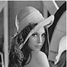
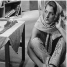
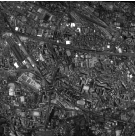
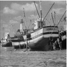
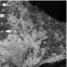
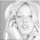
(a) Lena	(b) Barbara	(c) Marseille	(d) Boat	(e) Tunis	(f) Tiffany

Figure 2: Original images: (a) Lena, (b) Barbara, (c) Marseille, (d) Boat, (e) Tunis and (f) Tiffany.

VIII-B Numerical results

Table II provides the values of the SNR achieved by the different considered techniques for several values of the BSNR and a given form of blur (uniform $5\times 5$) on the six test images. All the provided quantitative results are median values computed over 10 noise realizations. It can be observed that, whatever the considered image is, SURE-based restoration methods generally lead to significant gains w.r.t. the other approaches, especially for low BSNRs. Furthermore, the two kinds of nonlinear estimating function which have been evaluated lead to almost identical results. It can also be noticed that the ForWaRD and TwIST methods perform quite well in terms of MSE for high BSNR. However, by examining more carefully the restored images, it can be seen that these methods may better recover uniform areas, at the expense of a loss of some detail information which is better preserved by the considered SURE-based method. This behaviour is visible on Fig. 3 where the proposed approach allows us to better recover Barbara’s stripe trouser.

Table III provides the SNRs obtained with the different techniques for several values of the $\mathrm{BSNR}$ and various blurs on Tunis image (see Fig. 2 (e)). The reported results allow us to confirm the good performance of SURE-based methods. The lower performance of the wavelet-based variational approach may be related to the fact that it requires the estimation of the hyperparameters of the prior distribution of the wavelet coefficients. This estimation has been performed by a maximum likelihood approach which is suboptimal in terms of mean square restoration error. The results at the bottom-right of Table III are in agreement with those in [29, 33] showing the outperformance of LET estimators for denoising problems. The poorer results obtained with ForWaRD in this case indicate that this method is tailored for deconvolution problems.

In the previous experiments, for all the considered methods, the noise variance $\gamma$ was assumed to be known. Table IV gives the SNR values obtained with the different techniques for several noise levels and various blurs on Tunis image, when the noise variance is estimated via the classical median absolute deviation (MAD) wavelet estimator [50, p. 447]. One can observe that the results are close to the case when the noise variance is known, except when the problem reduces to a denoising problem associated with a high BSNR. In this case indeed, the MAD estimator does not provide a precise estimation of the noise variance. However, the restoration results are still satisfactory.

TABLE II: Restoration results for a $5\times 5$ uniform blur: initial SNR ($\mathrm{SNR\_i}$) and SNR obtained with our approach using the nonlinear function in (49) ($\mathrm{SNR\_b}$), our approach using the nonlinear function in (50) ($\mathrm{SNR\_s}$), ForWaRD ($\mathrm{SNR\_f}$), TwIST ($\mathrm{SNR\_t}$), the wavelet-based variational approach ($\mathrm{SNR\_v}$), the Wiener filter ($\mathrm{SNR\_w}$) and the regularized quadratic method ($\mathrm{SNR\_r}$).

Image	BSNR	10	15	20	25	30	Image	BSNR	10	15	20	25	30
	SNR_i	9.796	14.26	17.89	20.21	21.31		SNR_i	9.713	14.03	17.39	19.39	20.28
	SNR_b	19.98	21.36	22.43	23.48	24.62		SNR_b	19.09	20.27	21.31	22.37	23.59
	SNR_s	19.93	21.29	22.39	23.45	24.58		SNR_s	19.05	20.22	21.27	22.36	23.57
Lena	SNR_f	18.27	20.04	21.36	23.35	24.63	Boat	SNR_f	16.75	19.05	20.68	22.14	23.49
	SNR_t	19.52	21.17	22.79	23.90	24.91		SNR_t	18.29	19.67	21.09	22.35	23.80
	SNR_v	17.91	20.01	21.34	22.41	23.42		SNR_v	14.37	17.46	19.31	20.54	21.88
	SNR_w	15.82	19.69	21.54	22.23	22.46		SNR_w	15.80	19.19	20.56	21.02	21.17
	SNR_r	18.70	20.06	21.25	22.18	22.43		SNR_r	18.18	19.31	20.35	20.96	21.15
	SNR_i	9.366	13.10	15.54	16.72	17.17		SNR_i	9.713	14.03	17.37	19.36	20.24
	SNR_b	17.02	17.54	18.05	18.79	19.75		SNR_b	18.63	19.73	20.75	21.72	22.66
	SNR_s	16.99	17.52	18.06	18.77	19.63		SNR_s	18.62	19.73	20.73	21.70	22.66
Barbara	SNR_f	16.14	17.04	17.62	18.56	19.49	Tunis	SNR_f	16.57	18.54	19.99	21.20	22.29
	SNR_t	16.74	17.45	17.95	18.38	19.07		SNR_t	18.03	18.94	20.35	21.50	22.56
	SNR_v	16.41	17.26	17.76	18.32	18.94		SNR_v	17.45	18.73	19.60	20.54	21.56
	SNR_w	14.53	16.92	17.78	18.02	18.10		SNR_w	15.80	19.07	20.37	20.79	20.92
	SNR_r	16.53	17.11	17.58	17.92	18.10		SNR_r	18.13	19.20	20.17	20.76	20.91
	SNR_i	8.926	11.93	13.57	14.25	14.49		SNR_i	9.923	14.73	19.15	22.72	24.95
	SNR_b	13.92	15.12	16.21	17.27	18.46		SNR_b	24.18	25.28	26.13	26.92	28.09
	SNR_s	13.93	15.12	16.21	17.28	18.48		SNR_s	24.16	25.24	26.11	26.92	28.09
Marseille	SNR_f	13.10	14.42	15.75	17.00	18.32	Tiffany	SNR_f	17.93	21.72	23.67	26.53	28.12
	SNR_t	12.74	14.19	15.52	16.87	18.36		SNR_t	23.08	25.17	26.23	27.20	27.85
	SNR_v	13.57	14.99	16.12	16.92	17.66		SNR_v	21.81	24.47	25.63	26.44	27.46
	SNR_w	12.60	14.70	15.53	15.81	15.90		SNR_w	18.01	23.13	25.48	26.28	26.53
	SNR_r	13.25	14.43	15.45	15.78	15.90		SNR_r	23.65	24.60	25.42	26.12	26.44

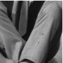
(a)	(b)

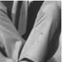
(c)	(d)	(e)

Figure 3: Zooms on Barbara image, $\mathrm{BSNR}=25$ dB; (a) Original, (b) Degraded, (c) Restored with ForWaRD, (d) Restored with TwIST and (e) Restored with the proposed method using (50).

TABLE III: Tunis image restoration for various blurs.

Blur	BSNR	10	15	20	25	30	Blur	BSNR	10	15	20	25	30
	SNR_i	9.662	13.86	17.01	18.80	19.56		SNR_i	9.577	13.64	16.56	18.13	18.77
	SNR_b	18.16	19.11	20.00	20.83	21.57		SNR_b	18.06	18.87	19.57	20.30	21.14
Gaussian	SNR_s	18.16	19.10	19.99	20.81	21.56	Uniform	SNR_s	18.05	18.86	19.57	20.29	21.14
$\sigma_{h}=2$	SNR_f	17.52	18.57	19.61	20.57	21.43	$7\times 7$	SNR_f	16.54	18.02	19.15	20.10	20.97
	SNR_t	17.12	18.32	19.47	20.40	21.33		SNR_t	17.39	18.21	19.22	20.04	20.94
	SNR_v	17.39	18.98	19.84	20.63	21.45		SNR_v	17.39	18.81	19.53	20.27	21.13
	SNR_w	16.24	18.70	19.49	19.57	19.62		SNR_w	16.06	18.45	19.11	19.28	19.33
	SNR_r	17.73	18.63	19.35	19.57	19.62		SNR_r	17.64	18.50	19.09	19.26	19.33
	SNR_i	9.971	14.87	19.57	23.74	26.83		SNR_i	10.00	15.00	20.00	25.00	30.00
	SNR_b	19.82	21.87	24.05	26.16	27.99		SNR_b	19.97	22.30	25.05	28.25	31.97
Cosine	SNR_s	19.82	21.85	24.02	26.13	27.98		SNR_s	19.96	22.27	25.02	28.20	31.91
$F_{c}=3/32$	SNR_f	17.94	19.85	22.48	24.79	26.82	Dirac	SNR_f	5.701	11.68	19.10	25.96	31.41
	SNR_t	18.52	21.18	23.81	25.94	27.78		SNR_t	19.82	22.03	24.27	27.18	31.00
	SNR_v	18.30	21.17	23.45	25.61	27.41		SNR_v	18.10	21.02	23.44	26.58	30.18
	SNR_w	12.63	17.50	21.98	25.61	27.89		SNR_w	10.42	15.13	20.04	25.01	30.00
	SNR_r	19.23	21.03	23.00	25.03	27.04		SNR_r	19.39	21.37	23.76	26.58	29.91

TABLE IV: Tunis image restoration for various blurs when the noise variance is estimated with the MAD estimator.

Blur	BSNR	10	15	20	25	30	Blur	BSNR	10	15	20	25	30
	SNR_i	9.662	13.86	17.01	18.80	19.56		SNR_i	9.577	13.64	16.56	18.13	18.77
Gaussian	SNR_b	18.16	19.12	20.00	20.82	21.57	Uniform	SNR_b	18.05	18.87	19.57	20.30	21.15
$\sigma_{h}=2$	SNR_s	18.15	19.11	19.99	20.81	21.56	$7\times 7$	SNR_s	18.05	18.86	19.57	20.30	21.15
	SNR_i	9.971	14.87	19.57	23.74	26.83		SNR_i	10.00	15.00	20.00	25.00	30.00
Cosine	SNR_b	19.82	21.87	24.05	26.15	27.99	Dirac	SNR_b	19.97	22.28	24.96	27.87	30.79
$F_{c}=3/32$	SNR_s	19.81	21.85	24.02	26.12	27.97		SNR_s	19.96	22.26	24.92	27.83	30.77

IX Conclusions

In this paper, we have addressed the problem of recovering data degraded by a convolution and the addition of a white Gaussian noise. We have adopted a hybrid approach that combines frequency and multiscale analyses. By formulating the underlying deconvolution problem as a nonlinear estimation problem, we have shown that the involved criterion to be optimized can be deduced from Stein’s unbiased quadratic risk estimate. In this context, attention must be paid to the variance of the risk estimate. The expression of this variance has been derived in this paper.

The flexibility of the proposed recovery approach must be emphasized. Redundant or non-redundant data representations can be employed as well as various combinations of linear/nonlinear estimates. Based on a specific choice of the wavelet representation and particular forms of the estimator structure, experiments have been conducted on a set of images, illustrating the good performance of the proposed approach. In our future work, we plan to further improve this restoration method by considering more sophisticated forms of the estimator, for example, by taking into account multiscale or spatial dependencies as proposed in [32, 34] for denoising problems. Furthermore, it seems interesting to extend this work to the case of multicomponent data by accounting for the cross-channel correlations.

Appendix A Proof of Proposition 2

We first notice that Assumption (ii) is a sufficient condition for the existence of the left hand-side terms of (10)-(13) since, by Hölder’s inequality,

$${\mathsf{E}}[|\Theta_{1}(\rho_{1})\widetilde{\eta}_{1}|]\leq {\mathsf{E}}[|\Theta_{1}(\rho_{1})|^{3}]^{1/3}{\mathsf{E}}[|\widetilde{\eta}_{1}|^{3/2}]^{2/3}$$ (52)

$${\mathsf{E}}[|\Theta_{1}(\rho_{1})\widetilde{\eta}_{1}\widetilde{\eta}_{2}|]\leq {\mathsf{E}}[|\Theta_{1}(\rho_{1})|^{3}]^{1/3}{\mathsf{E}}[|\widetilde{\eta}_{1}\widetilde{\eta}_{2}|^{3/2}]^{2/3}$$ (53)

$${\mathsf{E}}[|\Theta_{1}(\rho_{1})\widetilde{\eta}_{1}|\widetilde{\eta}_{2}^{2}]\leq {\mathsf{E}}[|\Theta_{1}(\rho_{1})|^{3}]^{1/3}{\mathsf{E}}[|\widetilde{\eta}_{1}|^{3/2}|\widetilde{\eta}_{2}|^{3}]^{2/3}$$ (54)

$${\mathsf{E}}[|\Theta_{1}(\rho_{1})\Theta_{1}(\rho_{2})\widetilde{\eta}_{1}\widetilde{\eta}_{2}|]\leq {\mathsf{E}}[|\Theta_{1}(\rho_{1})|^{3}]^{1/3}{\mathsf{E}}[|\Theta_{1}(\rho_{2})|^{3}]^{1/3}$$

$$\times{\mathsf{E}}[|\widetilde{\eta}_{1}\widetilde{\eta}_{2}|^{3}]^{1/3}.$$ (55)

We can decompose $\widetilde{\eta}_{i}$ with $i\in\{1,2\}$ as follows:

$$\widetilde{\eta}_{i}=a_{i}\eta_{1}+\check{\eta}_{i}$$ (56)

where $a_{i}$ is the mean-square prediction coefficient given by

$$\sigma^{2}a_{i}={\mathsf{E}}[\eta_{1}\widetilde{\eta}_{i}]$$ (57)

with $\sigma^{2}={\mathsf{E}}[\eta_{1}^{2}]$ and, $\check{\eta}_{i}$ is the associated zero-mean prediction error which is independent of $\upsilon_{1}$ and $\eta_{1}$. We deduce that

$${\mathsf{E}}[\Theta_{1}(\rho_{1})\widetilde{\eta}_{1}]=a_{1}{\mathsf{E}}[\Theta_{1}(\rho_{1})\eta_{1}].$$ (58)

We can invoke Stein’s principle to express ${\mathsf{E}}[\Theta_{1}(\rho_{1})\eta_{1}]$, provided that the assumptions in Proposition 1 are satisfied. To check these assumptions, we remark that, for every $\tau\in{\mathbb{R}}$, when $|\zeta|$ is large enough, $|\Theta_{1}(\tau+\zeta)|\exp\big{(}-\frac{\zeta^{2}}{2\sigma^{2}}\big{)}\leq|\Theta_{1}(\tau+\zeta)|\zeta^{2}\exp\big{(}-\frac{\zeta^{2}}{2\sigma^{2}}\big{)}$, which, owing to Assumption (i), implies that $\lim_{|\zeta|\to\infty}\Theta_{1}(\tau+\zeta)\exp\big{(}-\frac{\zeta^{2}}{2\sigma^{2}}\big{)}=0.$ In addition, from Jensen’s inequality and Assumption (ii), ${\mathsf{E}}[|\Theta_{1}^{\prime}(\rho_{1})|]\leq{\mathsf{E}}[|\Theta_{1}^{\prime}(\rho_{1})|^{3}]^{1/3}<\infty.$ Consequently, (9) combined with (57) can be applied to simplify (58), so allowing us to obtain (10).

Let us next prove (11). From (56), we get:

$${\mathsf{E}}[\Theta_{1}(\rho_{1})\widetilde{\eta}_{1}\widetilde{\eta}_{2}]= a_{1}a_{2}{\mathsf{E}}[\Theta_{1}(\rho_{1})\eta_{1}^{2}]+a_{1}{\mathsf{E}}[\Theta_{1}(\rho_{1})\eta_{1}]{\mathsf{E}}[\check{\eta}_{2}]$$

$$+a_{2}{\mathsf{E}}[\Theta_{1}(\rho_{1})\eta_{1}]{\mathsf{E}}[\check{\eta}_{1}]+{\mathsf{E}}[\Theta_{1}(\rho_{1})]{\mathsf{E}}[\check{\eta}_{1}\check{\eta}_{2}]$$

$$= a_{1}a_{2}{\mathsf{E}}[\Theta_{1}(\rho_{1})\eta_{1}^{2}]+{\mathsf{E}}[\Theta_{1}(\rho_{1})]{\mathsf{E}}[\check{\eta}_{1}\check{\eta}_{2}]$$ (59)

where we have used in the first equality the fact that $(\check{\eta}_{1},\check{\eta}_{2})$ is independent of $(\eta_{1},\upsilon_{1})$ and, in the second one, that it is zero-mean. Then, by making use of the orthogonality relation:

$${\mathsf{E}}[\widetilde{\eta}_{1}\widetilde{\eta}_{2}]=a_{1}a_{2}\sigma^{2}+{\mathsf{E}}[\check{\eta}_{1}\check{\eta}_{2}]$$ (60)

we have

$${\mathsf{E}}[\Theta_{1}(\rho_{1})\widetilde{\eta}_{1}\widetilde{\eta}_{2}]= a_{1}a_{2}\big{(}{\mathsf{E}}[\Theta_{1}(\rho_{1})\eta_{1}^{2}]-\sigma^{2}{\mathsf{E}}[\Theta_{1}(\rho_{1})]\big{)}$$

$$+{\mathsf{E}}[\Theta_{1}(\rho_{1})]{\mathsf{E}}[\widetilde{\eta}_{1}\widetilde{\eta}_{2}].$$ (61)

In addition, by integration by parts, the conditional expectation w.r.t. $\upsilon_{1}$ given by

$$\forall\tau,\qquad{\mathsf{E}}[\Theta_{1}(\rho_{1})\eta_{1}^{2}\mid\upsilon_{1}=\tau]=\\ \frac{1}{\sqrt{2\pi}\sigma}\int_{-\infty}^{\infty}\Theta_{1}(\tau+\zeta)\zeta^{2}\exp\big{(}-\frac{\zeta^{2}}{2\sigma^{2}}\big{)}\,d\zeta$$ (62)

can be reexpressed as

$${\mathsf{E}}[\Theta_{1}(\rho_{1})\eta_{1}^{2}\mid\upsilon_{1}=\tau]$$

$$= \frac{\sigma}{\sqrt{2\pi}}\Big{(}\lim_{\zeta\to-\infty}\Theta_{1}(\tau+\zeta)\zeta\exp\big{(}-\frac{\zeta^{2}}{2\sigma^{2}}\big{)}$$

$$-\lim_{\zeta\to\infty}\Theta_{1}(\tau+\zeta)\zeta\exp\big{(}-\frac{\zeta^{2}}{2\sigma^{2}}\big{)}$$

$$+\int_{-\infty}^{\infty}\big{(}\Theta_{1}(\tau+\zeta)+\Theta_{1}^{\prime}(\tau+\zeta)\zeta\big{)}\exp\big{(}-\frac{\zeta^{2}}{2\sigma^{2}}\big{)}\,d\zeta\Big{)}.$$ (63)

The existence of the latter integral is secured for almost every value $\tau$ that can be taken by $\upsilon_{1}$, thanks to Assumptions (ii) and (iii) and, the fact that, if $\mu$ denotes the probability measure of $\upsilon_{1}$,

$$\iint_{\mathbb{R}^{2}}\big{|}\Theta_{1}(\upsilon_{1}+\tau)+\Theta_{1}^{\prime}(\upsilon_{1}+\tau)\zeta\big{|}\exp\big{(}-\frac{\zeta^{2}}{2\sigma^{2}}\big{)}\,d\zeta d\mu(\tau)$$

$$= {\mathsf{E}}[|\Theta_{1}(\rho_{1})+\Theta_{1}^{\prime}(\rho_{1})\eta_{1}|]$$

$$\leq {\mathsf{E}}[|\Theta_{1}(\rho_{1})|]+{\mathsf{E}}[|\Theta_{1}^{\prime}(\rho_{1})\eta_{1}|]$$

$$\leq {\mathsf{E}}[|\Theta_{1}(\rho_{1})|^{3}]^{1/3}+{\mathsf{E}}[|\Theta_{1}^{\prime}(\rho_{1})|^{3}]^{1/3}{\mathsf{E}}[|\eta_{1}|^{3/2}]^{2/3}<\infty.$$ (64)

Since, for every $\tau\in{\mathbb{R}}$, when $|\zeta|$ is large enough, $|\Theta_{1}(\tau+\zeta)\zeta|\exp\big{(}-\frac{\zeta^{2}}{2\sigma^{2}}\big{)}\leq|\Theta_{1}(\tau+\zeta)|\zeta^{2}\exp\big{(}-\frac{\zeta^{2}}{2\sigma^{2}}\big{)}$, Assumption (i) implies that $\lim_{|\zeta|\to\infty}\Theta_{1}(\tau+\zeta)\zeta\exp\big{(}-\frac{\zeta^{2}}{2\sigma^{2}}\big{)}=0$. By using this property, we deduce from (63) that ${\mathsf{E}}[\Theta_{1}(\rho_{1})\eta_{1}^{2}\mid\upsilon_{1}]=\sigma^{2}\big{(}{\mathsf{E}}[\Theta_{1}(\upsilon_{1}+\eta_{1})\mid\upsilon_{1}]+{\mathsf{E}}[\Theta_{1}^{\prime}(\upsilon_{1}+\eta_{1})\eta_{1}\mid\upsilon_{1}]\big{)}$, which yields

$${\mathsf{E}}[\Theta_{1}(\rho_{1})\eta_{1}^{2}]=\sigma^{2}\big{(}{\mathsf{E}}[\Theta_{1}(\rho_{1})]+{\mathsf{E}}[\Theta_{1}^{\prime}(\rho_{1})\eta_{1}]\big{)}.$$ (65)

By inserting this equation in (61), we find that ${\mathsf{E}}[\Theta_{1}(\rho_{1})\widetilde{\eta}_{1}\widetilde{\eta}_{2}]=a_{1}a_{2}\sigma^{2}{\mathsf{E}}[\Theta_{1}^{\prime}(\rho_{1})\eta_{1}]+{\mathsf{E}}[\Theta_{1}(\rho_{1})]{\mathsf{E}}[\widetilde{\eta}_{1}\widetilde{\eta}_{2}].$ Formula (11) straightforwardly follows by noticing that, according to (56) and (57), ${\mathsf{E}}[\Theta_{1}^{\prime}(\rho_{1})\widetilde{\eta}_{2}]{\mathsf{E}}[\eta_{1}\widetilde{\eta}_{1}]=a_{1}a_{2}\sigma^{2}{\mathsf{E}}[\Theta_{1}^{\prime}(\rho_{1})\eta_{1}].$ Consider now (12). By using (56) and the independence between $(\check{\eta}_{1},\check{\eta}_{2})$ and $(\eta_{1},\upsilon_{1})$, we can write

$${\mathsf{E}}[\Theta_{1}(\rho_{1})\widetilde{\eta}_{1}\widetilde{\eta}_{2}^{2}]$$

$$= a_{1}a_{2}^{2}{\mathsf{E}}[\Theta_{1}(\rho_{1})\eta_{1}^{3}]+2a_{1}a_{2}{\mathsf{E}}[\Theta_{1}(\rho_{1})\eta_{1}^{2}]{\mathsf{E}}[\check{\eta}_{2}]$$

$$+a_{1}{\mathsf{E}}[\Theta_{1}(\rho_{1})\eta_{1}]{\mathsf{E}}[\check{\eta}_{2}^{2}]+a_{2}^{2}{\mathsf{E}}[\Theta_{1}(\rho_{1})\eta_{1}^{2}]{\mathsf{E}}[\check{\eta}_{1}]$$

$$+2a_{2}{\mathsf{E}}[\Theta_{1}(\rho_{1})\eta_{1}]{\mathsf{E}}[\check{\eta}_{1}\check{\eta}_{2}]+{\mathsf{E}}[\Theta_{1}(\rho_{1})]{\mathsf{E}}[\check{\eta}_{1}\check{\eta}_{2}^{2}]$$

$$= a_{1}a_{2}^{2}{\mathsf{E}}[\Theta_{1}(\rho_{1})\eta_{1}^{3}]+{\mathsf{E}}[\Theta_{1}(\rho_{1})\eta_{1}]\big{(}a_{1}{\mathsf{E}}[\check{\eta}_{2}^{2}]+2a_{2}{\mathsf{E}}[\check{\eta}_{1}\check{\eta}_{2}]\big{)}$$ (66)

where the latter equality stems from the symmetry of the probability distribution of $(\check{\eta}_{1},\check{\eta}_{2})$. Taking into account the relation ${\mathsf{E}}[\widetilde{\eta}_{2}^{2}]=a_{2}^{2}\sigma^{2}+{\mathsf{E}}[\check{\eta}_{2}^{2}]$ and (60), we get

$${\mathsf{E}}[\Theta_{1}(\rho_{1})\widetilde{\eta}_{1}\widetilde{\eta}_{2}^{2}]= a_{1}a_{2}^{2}\big{(}{\mathsf{E}}[\Theta_{1}(\rho_{1})\eta_{1}^{3}]-3\sigma^{2}{\mathsf{E}}[\Theta_{1}(\rho_{1})\eta_{1}]\big{)}$$

$$+{\mathsf{E}}[\Theta_{1}(\rho_{1})\eta_{1}]\big{(}a_{1}{\mathsf{E}}[\widetilde{\eta}_{2}^{2}]+2a_{2}{\mathsf{E}}[\widetilde{\eta}_{1}\widetilde{\eta}_{2}]\big{)}.$$ (67)

Let us now focus our attention on ${\mathsf{E}}[\Theta_{1}(\rho_{1})\eta_{1}^{3}]$. Since Assumptions (ii) and (iii) imply that

$${\mathsf{E}}[|2\Theta_{1}(\rho_{1})\eta_{1}+\Theta_{1}^{\prime}(\rho_{1})\eta_{1}^{2}|]\leq 2{\mathsf{E}}[|\Theta_{1}(\rho_{1})|^{3}]^{1/3}{\mathsf{E}}[|\eta_{1}|^{3/2}]^{2/3}\\ +{\mathsf{E}}[|\Theta_{1}^{\prime}(\rho_{1})|^{3}]^{1/3}{\mathsf{E}}[|\eta_{1}|^{3}]^{2/3}<\infty$$ (68)

and Assumption (i) holds, we can proceed by integration by parts, similarly to the proof of (65) to show that

$${\mathsf{E}}[\Theta_{1}(\rho_{1})\eta_{1}^{3}]=\sigma^{2}\big{(}2{\mathsf{E}}[\Theta_{1}(\rho_{1})\eta_{1}]+{\mathsf{E}}[\Theta_{1}^{\prime}(\rho_{1})\eta_{1}^{2}]\big{)}.$$ (69)

Thus, (66) reads

$${\mathsf{E}}[\Theta_{1}(\rho_{1})\widetilde{\eta}_{1}\widetilde{\eta}_{2}^{2}]= a_{1}a_{2}^{2}\sigma^{2}{\mathsf{E}}[\Theta_{1}^{\prime}(\rho_{1})\eta_{1}^{2}]+{\mathsf{E}}[\Theta_{1}(\rho_{1})\eta_{1}]$$

$$\times\big{(}a_{1}{\mathsf{E}}[\widetilde{\eta}_{2}^{2}]-a_{1}a_{2}^{2}\sigma^{2}+2a_{2}{\mathsf{E}}[\widetilde{\eta}_{1}\widetilde{\eta}_{2}]\big{)}$$ (70)

which, by using (9), can also be reexpressed as

$${\mathsf{E}}[\Theta_{1}(\rho_{1})\widetilde{\eta}_{1}\widetilde{\eta}_{2}^{2}]= a_{1}a_{2}^{2}\sigma^{2}{\mathsf{E}}[\Theta_{1}^{\prime}(\rho_{1})\eta_{1}^{2}]+\sigma^{2}{\mathsf{E}}[\Theta_{1}^{\prime}(\rho_{1})]$$

$$\times\big{(}a_{1}{\mathsf{E}}[\widetilde{\eta}_{2}^{2}]-a_{1}a_{2}^{2}\sigma^{2}+2a_{2}{\mathsf{E}}[\widetilde{\eta}_{1}\widetilde{\eta}_{2}]\big{)}.$$ (71)

In turn, we have

$${\mathsf{E}}[\Theta_{1}^{\prime}(\rho_{1})\widetilde{\eta}_{2}^{2}]= a_{2}^{2}{\mathsf{E}}[\Theta_{1}^{\prime}(\rho_{1})\eta_{1}^{2}]+2a_{2}{\mathsf{E}}[\Theta_{1}^{\prime}(\rho_{1})\eta_{1}]{\mathsf{E}}[\check{\eta}_{2}]$$

$$+{\mathsf{E}}[\Theta_{1}^{\prime}(\rho_{1})]{\mathsf{E}}[\check{\eta}_{2}^{2}]$$

$$= a_{2}^{2}{\mathsf{E}}[\Theta_{1}^{\prime}(\rho_{1})\eta_{1}^{2}]+{\mathsf{E}}[\Theta_{1}^{\prime}(\rho_{1})]\big{(}{\mathsf{E}}[\widetilde{\eta}_{2}^{2}]-a_{2}^{2}\sigma^{2}\big{)}$$ (72)

which, by using (57), leads to

$${\mathsf{E}}[\Theta_{1}^{\prime}(\rho_{1})\widetilde{\eta}_{2}^{2}]{\mathsf{E}}[\eta_{1}\widetilde{\eta}_{1}]= a_{1}a_{2}^{2}\sigma^{2}{\mathsf{E}}[\Theta_{1}^{\prime}(\rho_{1})\eta_{1}^{2}]$$

$$+\sigma^{2}{\mathsf{E}}[\Theta_{1}^{\prime}(\rho_{1})]a_{1}\big{(}{\mathsf{E}}[\widetilde{\eta}_{2}^{2}]-a_{2}^{2}\sigma^{2}\big{)}.$$ (73)

From the difference of (71) and (73), we derive that

$${\mathsf{E}}[\Theta_{1}(\rho_{1})\widetilde{\eta}_{1}\widetilde{\eta}_{2}^{2}]= {\mathsf{E}}[\Theta_{1}^{\prime}(\rho_{1})\widetilde{\eta}_{2}^{2}]{\mathsf{E}}[\eta_{1}\widetilde{\eta}_{1}]$$

$$+2a_{2}\sigma^{2}{\mathsf{E}}[\Theta_{1}^{\prime}(\rho_{1})]{\mathsf{E}}[\widetilde{\eta}_{1}\widetilde{\eta}_{2}]$$ (74)

which, by using again (57), yields (12).

Finally, we will prove Formula (13). We decompose $\widetilde{\eta}_{1}$ as follows:

$$\widetilde{\eta}_{1}=b\,\widetilde{\eta}_{2}+\widetilde{\eta}_{1}^{\perp}\qquad\text{where}\qquad b\,\widetilde{\sigma}^{2}={\mathsf{E}}[\widetilde{\eta}_{1}\widetilde{\eta}_{2}],$$ (75)

$\widetilde{\sigma}^{2}={\mathsf{E}}[\widetilde{\eta}_{2}^{2}]$ and, $\widetilde{\eta_{1}}^{\perp}$ is independent of $(\widetilde{\eta}_{2},\upsilon_{1},\upsilon_{2})$. This allows us to write

$${\mathsf{E}}[\Theta_{1}(\rho_{1})\Theta_{2}(\rho_{2})\widetilde{\eta}_{1}\widetilde{\eta}_{2}]=b\,{\mathsf{E}}[\Theta_{1}(\rho_{1})\Theta_{2}(\rho_{2})\widetilde{\eta}_{2}^{2}]\\ +{\mathsf{E}}[\Theta_{1}(\rho_{1})\Theta_{2}(\rho_{2})\widetilde{\eta}_{1}^{\perp}\widetilde{\eta}_{2}].$$ (76)

Let us first calculate ${\mathsf{E}}[\Theta_{1}(\rho_{1})\Theta(\rho_{2})\widetilde{\eta}_{2}^{2}]$. For $i\in\{1,2\}$, consider the decomposition:

$$\eta_{i}=c_{i}\widetilde{\eta}_{2}+\eta_{i}^{\perp}$$ (77)

where $c_{i}\widetilde{\sigma}^{2}={\mathsf{E}}[\eta_{i}\widetilde{\eta}_{2}]$ and, $\widetilde{\eta}_{2}$, $(\eta_{1}^{\perp},\eta_{2}^{\perp})$ and $(\upsilon_{1},\upsilon_{2})$ are independent. We have then

$${\mathsf{E}}[\Theta_{1}(\rho_{1})\Theta_{2}(\rho_{2})\widetilde{\eta}_{2}^{2}\mid\eta_{1}^{\perp},\eta_{2}^{\perp},\upsilon_{1},\upsilon_{2}]\\ =\frac{1}{\sqrt{2\pi}\widetilde{\sigma}}\int_{-\infty}^{\infty}\Theta_{1}(\upsilon_{1}+c_{1}\zeta+\eta_{1}^{\perp})\Theta_{2}(\upsilon_{2}+c_{2}\zeta+\eta_{2}^{\perp})\\ \times\zeta^{2}\exp\big{(}-\frac{\zeta^{2}}{2\widetilde{\sigma}^{2}}\big{)}\,d\zeta.$$ (78)

It can be noticed that

$${\mathsf{E}}[|\Theta_{1}(\rho_{1})\Theta_{2}(\rho_{2})+(c_{1}\Theta_{1}^{\prime}(\rho_{1})\Theta_{2}(\rho_{2})+c_{2}\Theta_{1}(\rho_{1})\Theta_{2}^{\prime}(\rho_{2}))\,\widetilde{\eta}_{2}|]$$

$$\leq{\mathsf{E}}[|\Theta_{1}(\rho_{1})|^{3}]^{1/3}{\mathsf{E}}[|\Theta_{2}(\rho_{2})|^{3}]^{1/3}+|c_{1}|\big{(}{\mathsf{E}}[|\Theta_{1}^{\prime}(\rho_{1})|^{3}]^{1/3}$$

$$\times{\mathsf{E}}[|\Theta_{2}(\rho_{2})|^{3}]^{1/3}+|c_{2}|{\mathsf{E}}[|\Theta_{1}(\rho_{1})|^{3}]^{1/3}{\mathsf{E}}[|\Theta_{2}^{\prime}(\rho_{2}))|^{3}]^{1/3}\big{)}$$

$$\times{\mathsf{E}}[|\widetilde{\eta}_{2}|^{3}]^{1/3}<\infty$$ (79)

and, for every $(\tau_{1},\tau_{2})\in{\mathbb{R}}^{2}$, $\lim_{|\zeta|\to\infty}\Theta_{1}(\tau_{1}+c_{1}\zeta)\Theta_{2}(\tau_{2}+c_{2}\zeta)\zeta\exp\big{(}-\frac{\zeta^{2}}{2\widetilde{\sigma}^{2}}\big{)}=0$ since, for $|\zeta|$ large enough,

$$c_{1}^{2}c_{2}^{2}|\Theta_{1}(\tau_{1}+c_{1}\zeta)\Theta_{2}(\tau_{2}+c_{2}\zeta)\zeta|\exp\big{(}-\frac{\zeta^{2}}{2\widetilde{\sigma}^{2}}\big{)}\\ \leq|\Theta_{1}(\tau_{1}+c_{1}\zeta)|(c_{1}\zeta)^{2}\exp\big{(}-\frac{\zeta^{2}}{4\widetilde{\sigma}^{2}}\big{)}\\ \times|\Theta_{2}(\tau_{2}+c_{2}\zeta)|(c_{2}\zeta)^{2}\exp\big{(}-\frac{\zeta^{2}}{4\widetilde{\sigma}^{2}}\big{)}$$ (80)

and Assumption (i) holds. We can therefore deduce, by integrating by parts in (78) and taking the expectation w.r.t. $(\eta_{1}^{\perp},\eta_{2}^{\perp},\upsilon_{1},\upsilon_{2})$, that

$${\mathsf{E}}[\Theta_{1}(\rho_{1})\Theta_{2}(\rho_{2})\widetilde{\eta}_{2}^{2}]$$

$$= \widetilde{\sigma}^{2}\big{(}{\mathsf{E}}[\Theta_{1}(\rho_{1})\Theta_{2}(\rho_{2})]+c_{1}{\mathsf{E}}[\Theta_{1}^{\prime}(\rho_{1})\Theta_{2}(\rho_{2})\,\widetilde{\eta}_{2}]$$

$$+c_{2}{\mathsf{E}}[\Theta_{1}(\rho_{1})\Theta_{2}^{\prime}(\rho_{2})\,\widetilde{\eta}_{2}]\big{)}$$

$$= \widetilde{\sigma}^{2}{\mathsf{E}}[\Theta_{1}(\rho_{1})\Theta_{2}(\rho_{2})]+{\mathsf{E}}[\Theta_{1}^{\prime}(\rho_{1})\Theta_{2}(\rho_{2})\,\widetilde{\eta}_{2}]{\mathsf{E}}[\eta_{1}\widetilde{\eta}_{2}]$$

$$+{\mathsf{E}}[\Theta_{1}(\rho_{1})\Theta_{2}^{\prime}(\rho_{2})\,\widetilde{\eta}_{2}]{\mathsf{E}}[\eta_{2}\widetilde{\eta}_{2}].$$ (81)

Let us now calculate ${\mathsf{E}}[\Theta_{1}(\rho_{1})\Theta_{2}(\rho_{2})\widetilde{\eta}_{1}^{\perp}\widetilde{\eta}_{2}]$. We have, for $i\in\{1,2\}$, $\eta_{i}=\check{c}_{i}\widetilde{\eta}_{1}^{\perp}+\check{\eta}_{i}^{\perp}$, where

$$\check{c_{i}}{\mathsf{E}}[(\widetilde{\eta}_{1}^{\perp})^{2}]={\mathsf{E}}[\eta_{i}\widetilde{\eta}_{1}^{\perp}]$$ (82)

and, $\widetilde{\eta}_{1}^{\perp}$ is independent of $(\widetilde{\eta}_{2},\check{\eta}_{1}^{\perp},\check{\eta}_{2}^{\perp},\upsilon_{1},\upsilon_{2})$. By proceeding similarly to the proof of (81), we get

$${\mathsf{E}}[\Theta_{1}(\rho_{1})\Theta_{2}(\rho_{2})\widetilde{\eta}_{1}^{\perp}\mid\widetilde{\eta}_{2},\check{\eta}_{1}^{\perp},\check{\eta}_{2}^{\perp}]={\mathsf{E}}[(\widetilde{\eta}_{1}^{\perp})^{2}]\\ \times\big{(}\check{c}_{1}{\mathsf{E}}[\Theta_{1}^{\prime}(\rho_{1})\Theta_{2}(\rho_{2})\mid\widetilde{\eta}_{2},\check{\eta}_{1}^{\perp},\check{\eta}_{2}^{\perp}]\\ +\check{c}_{2}{\mathsf{E}}[\Theta_{1}(\rho_{1})\Theta^{\prime}_{2}(\rho_{2})\mid\widetilde{\eta}_{2},\check{\eta}_{1}^{\perp},\check{\eta}_{2}^{\perp}]\big{)}$$ (83)

which, owing to (82), allows us to write

$${\mathsf{E}}[\Theta_{1}(\rho_{1})\Theta_{2}(\rho_{2})\widetilde{\eta}_{1}^{\perp}\widetilde{\eta}_{2}]= {\mathsf{E}}[\Theta_{1}^{\prime}(\rho_{1})\Theta_{2}(\rho_{2})\widetilde{\eta}_{2}]{\mathsf{E}}[\eta_{1}\widetilde{\eta}_{1}^{\perp}]$$

$$+{\mathsf{E}}[\Theta_{1}(\rho_{1})\Theta^{\prime}_{2}(\rho_{2})\widetilde{\eta}_{2}]{\mathsf{E}}[\eta_{2}\widetilde{\eta}_{1}^{\perp}].$$ (84)

On the other hand, from (75), we deduce that, for $i\in\{1,2\}$, ${\mathsf{E}}[\eta_{i}\widetilde{\eta}_{1}^{\perp}]={\mathsf{E}}[\eta_{i}\widetilde{\eta}_{1}]-b{\mathsf{E}}[\eta_{i}\widetilde{\eta}_{2}]$, so yielding

$${\mathsf{E}}[\Theta_{1}(\rho_{1})\Theta_{2}(\rho_{2})\widetilde{\eta}_{1}^{\perp}\widetilde{\eta}_{2}]= \,{\mathsf{E}}[\Theta_{1}^{\prime}(\rho_{1})\Theta_{2}(\rho_{2})\widetilde{\eta}_{2}]{\mathsf{E}}[\eta_{1}\widetilde{\eta}_{1}]$$

$$+{\mathsf{E}}[\Theta_{1}(\rho_{1})\Theta^{\prime}_{2}(\rho_{2})\widetilde{\eta}_{2}]{\mathsf{E}}[\eta_{2}\widetilde{\eta}_{1}]$$

$$-b\big{(}{\mathsf{E}}[\Theta_{1}^{\prime}(\rho_{1})\Theta_{2}(\rho_{2})\widetilde{\eta}_{2}]{\mathsf{E}}[\eta_{1}\widetilde{\eta}_{2}]$$

$$+{\mathsf{E}}[\Theta_{1}(\rho_{1})\Theta^{\prime}_{2}(\rho_{2})\widetilde{\eta}_{2}]{\mathsf{E}}[\eta_{2}\widetilde{\eta}_{2}]\big{)}.$$ (85)

Altogether, (76), (75), (81) and (85) lead to

$${\mathsf{E}}[\Theta_{1}(\rho_{1})\Theta_{2}(\rho_{2})\widetilde{\eta}_{1}\widetilde{\eta}_{2}]={\mathsf{E}}[\Theta_{1}(\rho_{1})\Theta_{2}(\rho_{2})]{\mathsf{E}}[\widetilde{\eta}_{1}\widetilde{\eta}_{2}]\\ +{\mathsf{E}}[\Theta_{1}^{\prime}(\rho_{1})\Theta_{2}(\rho_{2})\widetilde{\eta}_{2}]{\mathsf{E}}[\eta_{1}\widetilde{\eta}_{1}]+{\mathsf{E}}[\Theta_{1}(\rho_{1})\Theta^{\prime}_{2}(\rho_{2})\widetilde{\eta}_{2}]{\mathsf{E}}[\eta_{2}\widetilde{\eta}_{1}].$$ (86)

In order to obtain a more symmetric expression, let us now look at the difference ${\mathsf{E}}[\Theta_{1}(\rho_{1})\Theta^{\prime}_{2}(\rho_{2})\widetilde{\eta}_{2}]{\mathsf{E}}[\eta_{2}\widetilde{\eta}_{1}]-{\mathsf{E}}[\Theta_{1}(\rho_{1})\Theta^{\prime}_{2}(\rho_{2})\widetilde{\eta}_{1}]{\mathsf{E}}[\eta_{2}\widetilde{\eta}_{2}]={\mathsf{E}}[\Theta_{1}(\rho_{1})\Theta^{\prime}_{2}(\rho_{2})\widetilde{\eta}_{12}]$ where $\widetilde{\eta}_{12}={\mathsf{E}}[\eta_{2}\widetilde{\eta}_{1}]\widetilde{\eta}_{2}-{\mathsf{E}}[\eta_{2}\widetilde{\eta}_{2}]\widetilde{\eta}_{1}.$ Since $\widetilde{\eta}_{12}$ is a linear combination of $\widetilde{\eta}_{1}$ and $\widetilde{\eta}_{2}$ and, ${\mathsf{E}}[\eta_{2}\widetilde{\eta}_{12}]=0,$ $\widetilde{\eta}_{12}$ is independent of $(\eta_{2},\upsilon_{1},\upsilon_{2})$. Similarly to the derivation of Formula (10), it can be deduced that

$${\mathsf{E}}[\Theta_{1}(\rho_{1})\Theta^{\prime}_{2}(\rho_{2})\widetilde{\eta}_{12}\mid\eta_{2},\upsilon_{1},\upsilon_{2}]$$

$$= {\mathsf{E}}[\Theta_{1}(\rho_{1})\Theta^{\prime}_{2}(\upsilon_{2}+\eta_{2})\widetilde{\eta}_{12}\mid\eta_{2},\upsilon_{1},\upsilon_{2}]$$

$$= {\mathsf{E}}[\Theta_{1}(\rho_{1})\widetilde{\eta}_{12}\mid\eta_{2},\upsilon_{1},\upsilon_{2}]\,\Theta^{\prime}_{2}(\upsilon_{2}+\eta_{2})$$

$$= {\mathsf{E}}[\Theta_{1}^{\prime}(\rho_{1})\mid\eta_{2},\upsilon_{1},\upsilon_{2}]{\mathsf{E}}[\eta_{1}\widetilde{\eta}_{12}]\,\Theta^{\prime}_{2}(\rho_{2})$$ (87)

which leads to

$${\mathsf{E}}[\Theta_{1}(\rho_{1})\Theta^{\prime}_{2}(\rho_{2})\widetilde{\eta}_{2}]{\mathsf{E}}[\eta_{2}\widetilde{\eta}_{1}]-{\mathsf{E}}[\Theta_{1}(\rho_{1})\Theta^{\prime}_{2}(\rho_{2})\widetilde{\eta}_{1}]{\mathsf{E}}[\eta_{2}\widetilde{\eta}_{2}]$$

$$= {\mathsf{E}}[\Theta_{1}(\rho_{1})\Theta^{\prime}_{2}(\rho_{2})\widetilde{\eta}_{12}]={\mathsf{E}}[\Theta_{1}^{\prime}(\rho_{1})\Theta^{\prime}_{2}(\rho_{2})]{\mathsf{E}}[\eta_{1}\widetilde{\eta}_{12}]$$

$$= {\mathsf{E}}[\Theta_{1}^{\prime}(\rho_{1})\Theta^{\prime}_{2}(\rho_{2})]({\mathsf{E}}[\eta_{1}\widetilde{\eta}_{2}]{\mathsf{E}}[\eta_{2}\widetilde{\eta}_{1}]-{\mathsf{E}}[\eta_{1}\widetilde{\eta}_{1}]{\mathsf{E}}[\eta_{2}\widetilde{\eta}_{2}]).$$ (88)

Eq. (13) is then derived by combining (86) with (88).

Appendix B Proof of Proposition 3

We have, for every $\mathbf{p}\in\mathbb{D}$,

$${\mathsf{E}}[|\widetilde{R}(\mathbf{p})|^{2}]={\mathsf{E}}[|S(\mathbf{p})|^{2}]+{\mathsf{E}}[|\widetilde{N}(\mathbf{p})|^{2}]+2\,\mathrm{Re}\{{\mathsf{E}}[\widetilde{N}(\mathbf{p})\big{(}S(\mathbf{p})\big{)}^{*}]\}.$$ (89)

Since $\widetilde{n}$ and $s$ are uncorrelated, this yields ${\mathsf{E}}[|S(\mathbf{p})|^{2}]={\mathsf{E}}[|\widetilde{R}(\mathbf{p})|^{2}]-{\mathsf{E}}[|\widetilde{N}(\mathbf{p})|^{2}].$ In addition, we have ${\mathsf{E}}[S(\mathbf{p})\big{(}\widehat{S}(\mathbf{p})\big{)}^{*}]={\mathsf{E}}[\widetilde{R}(\mathbf{p})\big{(}\widehat{S}(\mathbf{p})\big{)}^{*}]-{\mathsf{E}}[\widetilde{N}(\mathbf{p})\big{(}\widehat{S}(\mathbf{p})\big{)}^{*}].$ The previous two equations show that

$$\forall\mathbf{p}\in\mathbb{D},\qquad {\mathsf{E}}[|\widehat{S}(\mathbf{p})-S(\mathbf{p})|^{2}]={\mathsf{E}}[|\widehat{S}(\mathbf{p})-\widetilde{R}(\mathbf{p})|^{2}]$$

$$- {\mathsf{E}}[|\widetilde{N}(\mathbf{p})|^{2}]+2\,\mathrm{Re}\{{\mathsf{E}}[\widetilde{N}(\mathbf{p})\big{(}\widehat{S}(\mathbf{p})\big{)}^{*}]\}.$$ (90)

Moreover, using (17), the second term in the right-hand side of (90) is

$${\mathsf{E}}[|\widetilde{N}(\mathbf{p})|^{2}]=\frac{\gamma D}{|H(\mathbf{p})|^{2}}.$$ (91)

On the other hand, according to (8), the last term in the right-hand side of (90) is such that

$${\mathsf{E}}[\widetilde{N}(\mathbf{p})\big{(}\widehat{S}(\mathbf{p})\big{)}^{*}]= \sum_{\mathbf{x}\in\mathbb{D}}\sum_{\ell=1}^{L}{\mathsf{E}}[\widehat{s}_{\ell}\,\widetilde{n}(\mathbf{x})]$$

$$\times\exp(-2\pi\imath{\mathbf{x}}^{\top}{\boldsymbol{D}}^{-1}{\mathbf{p}})\big{(}\widetilde{\Phi}_{\ell}({\mathbf{p}})\big{)}^{*}.$$ (92)

Furthermore, we know from (6) that $\widehat{s}_{\ell}=\Theta_{\ell}(u_{\ell}+n_{\ell})$, where

$$n_{\ell}=\langle n,\varphi_{\ell}\rangle,\qquad u_{\ell}=\langle u,\varphi_{\ell}\rangle$$ (93)

and, $u$ is the field in $\mathbb{R}^{D_{1}\times\cdots\times D_{d}}$ whose discrete Fourier coefficients are given by (3). From (93) as well as the assumptions made on the noise $n$ corrupting the data, it is clear that $\big{(}n_{\ell},\widetilde{n}(\mathbf{x})\big{)}$ is a zero-mean Gaussian vector which is independent of $u_{\ell}$. Thus, by using (10) in Proposition 2, we obtain:

$${\mathsf{E}}[\widehat{s}_{\ell}\widetilde{n}(\mathbf{x})]={\mathsf{E}}[\Theta^{\prime}_{\ell}(r_{\ell})]{\mathsf{E}}[n_{\ell}\,\widetilde{n}(\mathbf{x})].$$ (94)

Let us now calculate ${\mathsf{E}}[n_{\ell}\,\widetilde{n}(\mathbf{x})]$. Using (93) and (16), we get

$${\mathsf{E}}[n_{\ell}\,\widetilde{n}(\mathbf{x})]=\sum_{\mathbf{y}\in\mathbb{D}}{\mathsf{E}}[\widetilde{n}(\mathbf{x})\,n(\mathbf{y})]\varphi_{\ell}(\mathbf{y})$$

$$= \sum_{(\mathbf{p}^{\prime},\mathbf{p}^{\prime\prime})\in\mathbb{D}^{2}}{\mathsf{E}}\big{[}\widetilde{N}(\mathbf{p}^{\prime})\big{(}N(\mathbf{p}^{\prime\prime})\big{)}^{*}\big{]}\exp(2\pi\imath{\mathbf{x}}^{\top}{\boldsymbol{D}}^{-1}{\mathbf{p}^{\prime}})\frac{\Phi_{\ell}(\mathbf{p}^{\prime\prime})}{D^{2}}$$

$$= \frac{\gamma}{D}\sum_{\mathbf{p}^{\prime}\in\mathbb{D}}\frac{\Phi_{\ell}(\mathbf{p}^{\prime})}{H(\mathbf{p}^{\prime})}\exp(2\pi\imath{\mathbf{x}}^{\top}{\boldsymbol{D}}^{-1}{\mathbf{p}^{\prime}}).$$ (95)

Combining this equation with (92) and (94) yields

$${\mathsf{E}}[\widetilde{N}(\mathbf{p})\big{(}\widehat{S}(\mathbf{p})\big{)}^{*}]=\gamma\sum_{\ell=1}^{L}{\mathsf{E}}[\Theta^{\prime}_{\ell}(r_{\ell})]\frac{\Phi_{\ell}({\mathbf{p}})\big{(}\widetilde{\Phi}_{\ell}({\mathbf{p}})\big{)}^{*}}{H(\mathbf{p})}.$$ (96)

Gathering now (90), (91) and (96), (18) is obtained.

From Parseval’s formula, the global MSE can be expressed as

$$D\,{\mathsf{E}}[\mathcal{E}(\widehat{s}-s)]=\frac{1}{D}\sum_{\mathbf{p}\in\mathbb{D}}{\mathsf{E}}[|S(\mathbf{p})-\widehat{S}(\mathbf{p})|^{2}].$$ (97)

The above equation together with (18) show that (19) holds with

$$D\Delta=\gamma\Big{(}2\sum_{\ell=1}^{L}{\mathsf{E}}[\Theta_{\ell}^{\prime}(r_{\ell})]\,\mathrm{Re}\{\overline{\gamma}_{\ell}\}-\sum_{\mathbf{p}\in\mathbb{D}}|H(\mathbf{p})|^{-2}\Big{)}.$$ (98)

Furthermore, by defining

$$\forall\ell\in\{1,\ldots,L\},\qquad\widetilde{n}_{\ell}=\langle\widetilde{n},\widetilde{\varphi}_{\ell}\rangle$$ (99)

and using (16), it can be noticed that

$${\mathsf{E}}[n_{\ell}\,\widetilde{n}_{\ell}]=\sum_{(\mathbf{x},\mathbf{y})\in\mathbb{D}^{2}}{\mathsf{E}}[\widetilde{n}(\mathbf{y})n(\mathbf{x})]\widetilde{\varphi}_{\ell}(\mathbf{y})\varphi_{\ell}(\mathbf{x})$$

$$= \frac{1}{D^{2}}\sum_{(\mathbf{p},\mathbf{p^{\prime}})\in\mathbb{D}^{2}}{\mathsf{E}}\big{[}\widetilde{N}(\mathbf{p})\big{(}N(\mathbf{p}^{\prime})\big{)}^{*}\big{]}\big{(}\widetilde{\Phi}_{\ell}(\mathbf{p})\big{)}^{*}\Phi_{\ell}(\mathbf{p^{\prime}})$$

$$= \frac{\gamma}{D}\sum_{\mathbf{p}\in\mathbb{D}}\frac{\Phi_{\ell}({\mathbf{p}})\big{(}\widetilde{\Phi}_{\ell}({\mathbf{p}})\big{)}^{*}}{H(\mathbf{p})}=\gamma\overline{\gamma}_{\ell}.$$ (100)

Hence, as claimed in the last part of our statements, $(\overline{\gamma}_{\ell})_{1\leq\ell\leq L}$ is real-valued since it is the cross-correlation of a real-valued sequence.

Appendix C Proof of Proposition 5

By using (25), we have $\sum_{\mathbf{x}\in\mathbb{D}}\widehat{s}(\mathbf{x})\,\underline{\widetilde{n}}(\mathbf{x})=\sum_{\ell=1}^{L}\widehat{s}_{\ell}\,\widetilde{n}_{\ell}$, where $\widetilde{n}_{\ell}$ has been here redefined as

$$\widetilde{n}_{\ell}=\langle\widetilde{n},\underline{\widetilde{\varphi}}_{\ell}\rangle.$$ (101)

In addition, $\mathcal{E}(\underline{\widetilde{n}})=D^{-2}\sum_{\mathbf{p}\in\mathbb{Q}}|N(\mathbf{p})|^{2}/|H(\mathbf{p})|^{2}.$ This allows us to rewrite (34) as $\mathcal{E}_{o}-\widehat{\mathcal{E}}_{o}=-2A-B+2C$, where

$$A= \frac{1}{D}\sum_{\mathbf{x}\in\mathbb{D}}s(\mathbf{x})\,\underline{\widetilde{n}}(\mathbf{x})$$ (102)

$$B= \frac{1}{D}\sum_{\mathbf{x}\in\mathbb{D}}\big{(}\underline{\widetilde{n}}(\mathbf{x})\big{)}^{2}-\frac{\gamma}{D}\sum_{\mathbf{p}\in\mathbb{Q}}|H(\mathbf{p})|^{-2}$$

$$= \frac{1}{D}\sum_{\mathbf{p}\in\mathbb{Q}}\frac{|N(\mathbf{p})|^{2}/D-\gamma}{|H(\mathbf{p})|^{2}}$$ (103)

$$C= \frac{1}{D}\sum_{\ell=1}^{L}\big{(}\widehat{s}_{\ell}\,\widetilde{n}_{\ell}-\Theta_{\ell}^{\prime}(r_{\ell})\gamma\overline{\gamma}_{\ell}\big{)}.$$ (104)

The variance of the error in the estimation of the risk is thus given by

$$\mathsf{Var}[\mathcal{E}_{o}-\widehat{\mathcal{E}}_{o}]={\mathsf{E}}[(\mathcal{E}_{o}-\widehat{\mathcal{E}}_{o})^{2}]=4{\mathsf{E}}[A^{2}]+4{\mathsf{E}}[AB]-8{\mathsf{E}}[AC]\\ +{\mathsf{E}}[B^{2}]-4{\mathsf{E}}[BC]+4{\mathsf{E}}[C^{2}].$$ (105)

We will now calculate each of the terms in the right hand-side term of the above expression to determine the variance.

• Due to the independence of $s$ and $n$, the first term to calculate is equal to

  $${\mathsf{E}}[A^{2}]=\frac{1}{D^{4}}\sum_{(\mathbf{p},\mathbf{p}^{\prime})\in\mathbb{Q}^{2}}{\mathsf{E}}[S(\mathbf{p})\big{(}S(\mathbf{p}^{\prime})\big{)}^{*}]\,{\mathsf{E}}[\widetilde{N}(\mathbf{p})\big{(}\widetilde{N}(\mathbf{p}^{\prime})\big{)}^{*}].$$ (106)

  By using (17), this expression simplifies as

  $${\mathsf{E}}[A^{2}]=\frac{\gamma}{D^{3}}\sum_{\mathbf{p}\in\mathbb{Q}}\frac{{\mathsf{E}}[|S(\mathbf{p})|^{2}]}{|H(\mathbf{p})|^{2}}.$$ (107)

• The second term cancels. Indeed, since $n$ and hence $\underline{\widetilde{n}}$ are zero-mean,

  $${\mathsf{E}}[AB]=\frac{1}{D^{2}}\sum_{(\mathbf{x},\mathbf{x}^{\prime})\in\mathbb{D}^{2}}{\mathsf{E}}[s(\mathbf{x})]{\mathsf{E}}[\underline{\widetilde{n}}(\mathbf{x})\big{(}\underline{\widetilde{n}}(\mathbf{x}^{\prime}))^{2}].$$ (108)

  and, since $(\underline{\widetilde{n}}(\mathbf{x}),\underline{\widetilde{n}}(\mathbf{x}^{\prime}))$ is zero-mean Gaussian, it has a symmetric distribution and ${\mathsf{E}}[\underline{\widetilde{n}}(\mathbf{x})\big{(}\underline{\widetilde{n}}(\mathbf{x}^{\prime}))^{2}]=0$.

• The calculation of the third term is a bit more involved. We have

  $${\mathsf{E}}[AC]=\frac{1}{D^{2}}\sum_{\mathbf{x}\in\mathbb{D}}\sum_{\ell=1}^{L}\big{(}{\mathsf{E}}[s(\mathbf{x})\widehat{s}_{\ell}\,\widetilde{n}_{\ell}\,\underline{\widetilde{n}}(\mathbf{x})]\\ -{\mathsf{E}}[s(\mathbf{x})\Theta^{\prime}_{\ell}(r_{\ell})\underline{\widetilde{n}}(\mathbf{x})]\gamma\overline{\gamma}_{\ell}\big{)}.$$ (109)

  In order to find a tractable expression of ${\mathsf{E}}[s(\mathbf{x})\widehat{s}_{\ell}\,\widetilde{n}_{\ell}\,\underline{\widetilde{n}}(\mathbf{x})]$ with $\ell\in\{1,\ldots,L\}$, we will first consider the following conditional expectation w.r.t. $s$: ${\mathsf{E}}[s(\mathbf{x})\widehat{s}_{\ell}\,\widetilde{n}_{\ell}\,\underline{\widetilde{n}}(\mathbf{x})\mid s]=s(\mathbf{x})\,{\mathsf{E}}[\Theta(r_{\ell})\widetilde{n}_{\ell}\,\underline{\widetilde{n}}(\mathbf{x})\mid s].$ According to Formula (11) in Proposition 2,

  $${\mathsf{E}}[\Theta(r_{\ell})\widetilde{n}_{\ell}\,\underline{\widetilde{n}}(\mathbf{x})\mid s]= {\mathsf{E}}[\Theta^{\prime}_{\ell}(r_{\ell})\underline{\widetilde{n}}(\mathbf{x})\mid s]\,{\mathsf{E}}[n_{\ell}\,\widetilde{n}_{\ell}]$$

  $$+{\mathsf{E}}[\Theta_{\ell}(r_{\ell})\mid s]\,{\mathsf{E}}[\widetilde{n}_{\ell}\,\underline{\widetilde{n}}(\mathbf{x})]$$ (110)

  which, by using (100), allows us to deduce that

  $${\mathsf{E}}[s(\mathbf{x})\Theta(r_{\ell})\widetilde{n}_{\ell}\,\underline{\widetilde{n}}(\mathbf{x})]={\mathsf{E}}[s(\mathbf{x})\Theta^{\prime}_{\ell}(r_{\ell})\underline{\widetilde{n}}(\mathbf{x})]\,\gamma\overline{\gamma}_{\ell}\\ +{\mathsf{E}}[s(\mathbf{x})\Theta_{\ell}(r_{\ell})]\,{\mathsf{E}}[\widetilde{n}_{\ell}\,\underline{\widetilde{n}}(\mathbf{x})].$$ (111)

  This shows that (109) can be simplified as follows:

  $${\mathsf{E}}[AC]=\frac{1}{D^{2}}\sum_{\mathbf{x}\in\mathbb{D}}\sum_{\ell=1}^{L}{\mathsf{E}}[s(\mathbf{x})\Theta_{\ell}(r_{\ell})]\,{\mathsf{E}}[\widetilde{n}_{\ell}\,\underline{\widetilde{n}}(\mathbf{x})].$$ (112)

  Furthermore, according to (17) and (101), we have

  $${\mathsf{E}}[\widetilde{n}_{\ell}\,\underline{\widetilde{n}}(\mathbf{x})]= \frac{1}{D^{2}}\sum_{(\mathbf{p},\mathbf{p}^{\prime})\in\mathbb{Q}^{2}}{\mathsf{E}}[\widetilde{N}(\mathbf{p})\big{(}\widetilde{N}(\mathbf{p}^{\prime})\big{)}^{*}]\big{(}\widetilde{\Phi}_{\ell}(\mathbf{p})\big{)}^{*}$$

  $$\times\exp(-2\pi\imath{\mathbf{x}}^{\top}{\boldsymbol{D}}^{-1}{\mathbf{p}}^{\prime})$$

  $$= \frac{\gamma}{D}\sum_{\mathbf{p}\in\mathbb{Q}}\frac{\big{(}\widetilde{\Phi}_{\ell}(\mathbf{p})\big{)}^{*}}{|H(\mathbf{p})|^{2}}\exp(-2\pi\imath{\mathbf{x}}^{\top}{\boldsymbol{D}}^{-1}{\mathbf{p}}).$$ (113)

  This yields

  $${\mathsf{E}}[AC] =\frac{\gamma}{D^{3}}\sum_{\mathbf{p}\in\mathbb{Q}}\sum_{\ell=1}^{L}\frac{\big{(}\widetilde{\Phi}_{\ell}(\mathbf{p})\big{)}^{*}}{|H(\mathbf{p})|^{2}}{\mathsf{E}}[S(\mathbf{p})\Theta_{\ell}(r_{\ell})]$$

  $$=\frac{\gamma}{D^{3}}\sum_{\mathbf{p}\in\mathbb{Q}}\frac{{\mathsf{E}}[S(\mathbf{p})\big{(}\widehat{S}(\mathbf{p})\big{)}^{*}]}{|H(\mathbf{p})|^{2}}.$$ (114)

• The calculation of the fourth term is more classical since $|N(\mathbf{p})|^{2}/D$ is the $\mathbf{p}$ bin of the periodogram [51] of the Gaussian white noise $n$. More precisely, since $|N(\mathbf{p})|^{2}/D$ is an unbiased estimate of $\gamma$,

  $${\mathsf{E}}[B^{2}]=\frac{1}{D^{4}}\sum_{(\mathbf{p},\mathbf{p}^{\prime})\in\mathbb{Q}^{2}}\frac{\mathsf{Cov}(|N(\mathbf{p})|^{2},|N(\mathbf{p}^{\prime})|^{2})}{|H(\mathbf{p})|^{2}|H(\mathbf{p}^{\prime})|^{2}}.$$ (115)

  In the above summation, we know that, if $\mathbf{p}\neq\mathbf{p}^{\prime}$ and $\mathbf{p}\neq{\boldsymbol{D}}\mathbf{1}-\mathbf{p}^{\prime}$ with $\mathbf{1}=(1,\ldots,1)^{\top}\in{\mathbb{R}}^{d}$, $N(\mathbf{p})$ and $N(\mathbf{p}^{\prime})$ are independent and thus, $\mathsf{Cov}(|N(\mathbf{p})|^{2},|N(\mathbf{p}^{\prime})|^{2})=0$. On the other hand, if $\mathbf{p}=\mathbf{p}^{\prime}$ or $\mathbf{p}={\boldsymbol{D}}\mathbf{1}-\mathbf{p}^{\prime}$, then $\mathsf{Cov}(|N(\mathbf{p})|^{2},|N(\mathbf{p}^{\prime})|^{2})={\mathsf{E}}[|N(\mathbf{p})|^{4}]-\gamma^{2}D^{2}$. Let

  $$\mathbb{S}=\big{\{}\mathbf{p}=(p_{1},\ldots,p_{d})^{\top}\in\mathbb{D}\mid\\ \forall i\in\{1,\ldots,d\},p_{i}\in\{0,D_{i}/2\}\big{\}}.$$ (116)

  If $\mathbf{p}\in\mathbb{S}$, then $N(\mathbf{p})$ is a zero-mean Gaussian real random variable and ${\mathsf{E}}[|N(\mathbf{p})|^{4}]=3{\mathsf{E}}\big{[}\big{(}N(\mathbf{p})\big{)}^{2}\big{]}^{2}=3\gamma^{2}D^{2}$. Otherwise, $N(\mathbf{p})$ a zero-mean Gaussian circular complex random variable and ${\mathsf{E}}[|N(\mathbf{p})|^{4}]=2{\mathsf{E}}[|N(\mathbf{p})|^{2}]^{2}$ $=2\gamma^{2}D^{2}$. It can be deduced that

  $${\mathsf{E}}[B^{2}]= \frac{1}{D^{4}}\left(\sum_{\mathbf{p}\in\mathbb{Q}\cap\mathbb{S}}\frac{\mathsf{Var}[\big{(}N(\mathbf{p})\big{)}^{2}]}{|H(\mathbf{p})|^{4}}\right.$$

  $$+\sum_{\mathbf{p}\in\mathbb{Q}\cap(\mathbb{D}\setminus\mathbb{S})}\Big{(}\frac{\mathsf{Var}[\big{|}N(\mathbf{p})\big{|}^{2}]}{|H(\mathbf{p})|^{4}}$$

  $$\left.+\frac{\mathsf{Cov}(|N(\mathbf{p})|^{2},|N({\boldsymbol{D}}\mathbf{1}-\mathbf{p})|^{2})}{|H(\mathbf{p})|^{2}|H({\boldsymbol{D}}\mathbf{1}-\mathbf{p})|^{2}}\Big{)}\right)$$

  $$= \frac{1}{D^{4}}\left(\sum_{\mathbf{p}\in\mathbb{Q}\cap\mathbb{S}}\frac{2\gamma^{2}D^{2}}{|H(\mathbf{p})|^{4}}\right.$$

  $$\left.+\sum_{\mathbf{p}\in\mathbb{Q}\cap(\mathbb{D}\setminus\mathbb{S})}\Big{(}\frac{\gamma^{2}D^{2}}{|H(\mathbf{p})|^{4}}+\frac{\gamma^{2}D^{2}}{|H(\mathbf{p})|^{4}}\Big{)}\right)$$

  $$= \frac{2\gamma^{2}}{D^{2}}\sum_{\mathbf{p}\in\mathbb{Q}}\frac{1}{|H(\mathbf{p})|^{4}}.$$ (117)

• Let us now turn our attention to the fifth term. According to (10) and the definition of $\overline{\gamma}_{\ell}$ in (100), for every $\ell\in\{1,\ldots,L\}$, $\widehat{s}_{\ell}\,\widetilde{n}_{\ell}-\Theta_{\ell}^{\prime}(r_{\ell})\gamma\overline{\gamma}_{\ell}$ is zero-mean and we have then

  $${\mathsf{E}}[BC]=\frac{1}{D^{2}}\sum_{\mathbf{x}\in\mathbb{D}}\sum_{\ell=1}^{L}\Big{(}{\mathsf{E}}[\widehat{s}_{\ell}\,\widetilde{n}_{\ell}\big{(}\underline{\widetilde{n}}(\mathbf{x})\big{)}^{2}]\\ -{\mathsf{E}}[\Theta_{\ell}^{\prime}(r_{\ell})\big{(}\underline{\widetilde{n}}(\mathbf{x})\big{)}^{2}]\gamma\overline{\gamma}_{\ell}\Big{)}.$$ (118)

  By applying now Formula (12) in Proposition 2, we have, for every $\ell\in\{1,\ldots,L\}$,

  $${\mathsf{E}}[\widehat{s}_{\ell}\,\widetilde{n}_{\ell}\big{(}\underline{\widetilde{n}}(\mathbf{x})\big{)}^{2}]-{\mathsf{E}}[\Theta_{\ell}^{\prime}(r_{\ell})\big{(}\underline{\widetilde{n}}(\mathbf{x})\big{)}^{2}]\gamma\overline{\gamma}_{\ell}$$

  $$= {\mathsf{E}}[\Theta_{\ell}(r_{\ell})\,\widetilde{n}_{\ell}\big{(}\underline{\widetilde{n}}(\mathbf{x})\big{)}^{2}]-{\mathsf{E}}[\Theta_{\ell}^{\prime}(r_{\ell})\big{(}\widetilde{n}(\mathbf{x})\big{)}^{2}]\,{\mathsf{E}}[n_{\ell}\,\widetilde{n}_{\ell}]$$

  $$= 2{\mathsf{E}}[\Theta_{\ell}^{\prime}(r_{\ell})]\,{\mathsf{E}}[\widetilde{n}_{\ell}\,\underline{\widetilde{n}}(\mathbf{x})]\,{\mathsf{E}}[\underline{\widetilde{n}}(\mathbf{x})\,n_{\ell}]$$ (119)

  where, in compliance with (24), $n_{\ell}$ is now given by

  $$n_{\ell}=\langle\underline{n},\varphi_{\ell}\rangle.$$ (120)

  Furthermore, similarly to (95), we have

  $${\mathsf{E}}[\underline{\widetilde{n}}(\mathbf{x})\,n_{\ell}]= \frac{1}{D^{2}}\sum_{(\mathbf{p},\mathbf{p}^{\prime})\in\mathbb{Q}^{2}}{\mathsf{E}}[\widetilde{N}(\mathbf{p})\big{(}N(\mathbf{p}^{\prime})\big{)}^{*}]\Phi_{\ell}(\mathbf{p}^{\prime})$$

  $$\times\exp(2\pi\imath{\mathbf{x}}^{\top}{\boldsymbol{D}}^{-1}{\mathbf{p}})$$

  $$= \frac{\gamma}{D}\sum_{\mathbf{p}^{\prime}\in\mathbb{Q}}\frac{\Phi_{\ell}(\mathbf{p}^{\prime})}{H(\mathbf{p}^{\prime})}\exp(2\pi\imath{\mathbf{x}}^{\top}{\boldsymbol{D}}^{-1}{\mathbf{p}^{\prime}}).$$ (121)

  Altogether, (113), (119) and (121) yield

  $${\mathsf{E}}[\widehat{s}_{\ell}\,\widetilde{n}_{\ell}\big{(}\underline{\widetilde{n}}(\mathbf{x})\big{)}^{2}]-{\mathsf{E}}[\Theta_{\ell}^{\prime}(r_{\ell})\big{(}\underline{\widetilde{n}}(\mathbf{x})\big{)}^{2}]\gamma\overline{\gamma}_{\ell}\\ =\frac{2\gamma^{2}}{D^{2}}{\mathsf{E}}[\Theta_{\ell}^{\prime}(r_{\ell})]\sum_{(\mathbf{p},\mathbf{p}^{\prime})\in\mathbb{Q}^{2}}\frac{\Phi_{\ell}(\mathbf{p}^{\prime})\big{(}\widetilde{\Phi}_{\ell}(\mathbf{p})\big{)}^{*}}{H(\mathbf{p}^{\prime})|H(\mathbf{p})|^{2}}\\ \times\exp\big{(}2\pi\imath{\mathbf{x}}^{\top}{\boldsymbol{D}}^{-1}({\mathbf{p}^{\prime}}-\mathbf{p})\big{)}.$$ (122)

  Hence, (118) can be reexpressed as

  $${\mathsf{E}}[BC] =\frac{2\gamma^{2}}{D^{2}}\sum_{\ell=1}^{L}{\mathsf{E}}[\Theta_{\ell}^{\prime}(r_{\ell})]\,\kappa_{\ell}$$ (123)

  where

  $$\kappa_{\ell}=\frac{1}{D}\sum_{\mathbf{p}\in\mathbb{Q}}\frac{\Phi_{\ell}(\mathbf{p})\big{(}\widetilde{\Phi}_{\ell}(\mathbf{p})\big{)}^{*}}{H(\mathbf{p})|H(\mathbf{p})|^{2}}.$$ (124)

• Let us now consider the last term

  $${\mathsf{E}}[C^{2}]=\frac{1}{D^{2}}\sum_{\ell=1}^{L}\sum_{i=1}^{L}\big{(}{\mathsf{E}}[\widehat{s}_{\ell}\widehat{s}_{i}\widetilde{n}_{\ell}\widetilde{n}_{i}]-{\mathsf{E}}[\widehat{s}_{i}\Theta_{\ell}^{\prime}(r_{\ell})\,\widetilde{n}_{i}]\gamma\overline{\gamma}_{\ell}\\ -{\mathsf{E}}[\widehat{s}_{\ell}\Theta_{i}^{\prime}(r_{i})\,\widetilde{n}_{\ell}]\gamma\overline{\gamma}_{i}+{\mathsf{E}}[\Theta_{\ell}^{\prime}(r_{\ell})\Theta_{i}^{\prime}(r_{i})]\gamma^{2}\overline{\gamma}_{\ell}\overline{\gamma}_{i}\big{)}.$$ (125)

  Appealing to Formula (13) in Proposition 2 and (100), we have

  $${\mathsf{E}}[\Theta_{\ell}(r_{\ell})\Theta_{i}(r_{i})\widetilde{n}_{\ell}\widetilde{n}_{i}]$$

  $$= \,{\mathsf{E}}[\Theta_{\ell}(r_{\ell})\Theta_{i}(r_{i})]{\mathsf{E}}[\widetilde{n}_{\ell}\widetilde{n}_{i}]+{\mathsf{E}}[\Theta_{\ell}^{\prime}(r_{\ell})\Theta_{i}(r_{i})\widetilde{n}_{i}]\gamma\overline{\gamma}_{\ell}$$

  $$+{\mathsf{E}}[\Theta_{\ell}(r_{\ell})\Theta^{\prime}_{i}(r_{i})\widetilde{n}_{\ell}]\gamma\overline{\gamma}_{i}+{\mathsf{E}}[\Theta_{\ell}^{\prime}(r_{\ell})\Theta^{\prime}_{i}(r_{i})]$$

  $$\times({\mathsf{E}}[n_{i}\widetilde{n}_{\ell}]{\mathsf{E}}[\eta_{\ell}\widetilde{n}_{i}]-\gamma^{2}\overline{\gamma}_{\ell}\overline{\gamma}_{i}).$$ (126)

  This allows us to simplify (125) as follows:

  $${\mathsf{E}}[C^{2}]= \frac{1}{D^{2}}\sum_{\ell=1}^{L}\sum_{i=1}^{L}\big{(}{\mathsf{E}}[\widehat{s}_{\ell}\widehat{s}_{i}]{\mathsf{E}}[\widetilde{n}_{\ell}\widetilde{n}_{i}]$$

  $$+{\mathsf{E}}[\Theta_{\ell}^{\prime}(r_{\ell})\Theta_{i}^{\prime}(r_{i})]{\mathsf{E}}[n_{i}\widetilde{n}_{\ell}]{\mathsf{E}}[\eta_{\ell}\widetilde{n}_{i}]\big{)}.$$ (127)

  Furthermore, according to (17), (101), (16) and (120), we have

  $${\mathsf{E}}[\widetilde{n}_{\ell}\widetilde{n}_{i}] =\frac{1}{D^{2}}\sum_{(\mathbf{p},\mathbf{p}^{\prime})\in\mathbb{Q}^{2}}{\mathsf{E}}[\widetilde{N}(\mathbf{p})\big{(}\widetilde{N}(\mathbf{p}^{\prime})\big{)}^{*}]\big{(}\widetilde{\Phi}_{\ell}(\mathbf{p})\big{)}^{*}\widetilde{\Phi}_{i}(\mathbf{p}^{\prime})$$

  $$=\frac{\gamma}{D}\sum_{\mathbf{p}\in\mathbb{Q}}\frac{\big{(}\widetilde{\Phi}_{\ell}(\mathbf{p})\big{)}^{*}\widetilde{\Phi}_{i}(\mathbf{p})}{|H(\mathbf{p})|^{2}}$$ (128)

  and

  $${\mathsf{E}}[n_{\ell}\widetilde{n}_{i}]= \frac{1}{D^{2}}\sum_{(\mathbf{p},\mathbf{p}^{\prime})\in\mathbb{Q}^{2}}{\mathsf{E}}[\widetilde{N}(\mathbf{p})\big{(}N(\mathbf{p}^{\prime})\big{)}^{*}]\Phi_{\ell}(\mathbf{p}^{\prime})\big{(}\widetilde{\Phi}_{i}(\mathbf{p})\big{)}^{*}$$

  $$=\gamma\overline{\gamma}_{\ell,i}$$ (129)

  where the expression of $\overline{\gamma}_{\ell,i}$ is given by (37). Hence, by using (128)-(129), (127) can be rewritten as

  $${\mathsf{E}}[C^{2}]= \frac{\gamma}{D^{3}}\sum_{\mathbf{p}\in\mathbb{Q}}\frac{{\mathsf{E}}[|\widehat{S}(\mathbf{p})|^{2}]}{|H(\mathbf{p})|^{2}}$$

  $$+\frac{\gamma^{2}}{D^{2}}\sum_{\ell=1}^{L}\ \sum_{i=1}^{L}{\mathsf{E}}[\Theta_{\ell}^{\prime}(r_{\ell})\Theta_{i}^{\prime}(r_{i})]\overline{\gamma}_{\ell,i}\overline{\gamma}_{i,\ell}.$$ (130)

• In conclusion, we deduce from (105), (107), (114), (117), (123) and (130) that

  $$\mathsf{Var}[\mathcal{E}_{o} -\widehat{\mathcal{E}}_{o}]=\frac{4\gamma}{D^{3}}\sum_{\mathbf{p}\in\mathbb{Q}}\frac{{\mathsf{E}}[|\widehat{S}(\mathbf{p})-S(\mathbf{p})|^{2}]}{|H(\mathbf{p})|^{2}}$$

  $$+\frac{4\gamma^{2}}{D^{2}}\Big{(}\sum_{\ell=1}^{L}\ \sum_{i=1}^{L}{\mathsf{E}}[\Theta_{\ell}^{\prime}(r_{\ell})\Theta_{i}^{\prime}(r_{i})]\overline{\gamma}_{\ell,i}\overline{\gamma}_{i,\ell}$$

  $$-2\sum_{\ell=1}^{L}{\mathsf{E}}[\Theta_{\ell}^{\prime}(r_{\ell})]\kappa_{\ell}+\frac{1}{2}\sum_{\mathbf{p}\in\mathbb{Q}}\frac{1}{|H(\mathbf{p})|^{4}}\Big{)}.$$ (131)

  By exploiting now (18) (see Proposition 4) and noticing that $(\kappa_{\ell})_{1\leq\ell\leq L}$ is real-valued, this expression can be simplified as follows:

  $$\mathsf{Var}[\mathcal{E}_{o}-\widehat{\mathcal{E}}_{o}]=\frac{4\gamma}{D^{3}}\sum_{\mathbf{p}\in\mathbb{Q}}\frac{{\mathsf{E}}[|\widehat{S}(\mathbf{p})-\widetilde{R}(\mathbf{p})|^{2}]}{|H(\mathbf{p})|^{2}}\\ +\frac{4\gamma^{2}}{D^{2}}\sum_{\ell=1}^{L}\ \sum_{i=1}^{L}{\mathsf{E}}[\Theta_{\ell}^{\prime}(r_{\ell})\Theta_{i}^{\prime}(r_{i})]\overline{\gamma}_{\ell,i}\overline{\gamma}_{i,\ell}\\ -\frac{2\gamma^{2}}{D^{2}}\sum_{\mathbf{p}\in\mathbb{Q}}\frac{1}{|H(\mathbf{p})|^{4}}.$$ (132)

  Eq. (35) follows by using Parseval’s formula.

References

• [1] A. Benazza-Benyahia and J.- C. Pesquet, “A SURE approach for image deconvolution in an orthonormal wavelet basis,” International Symposium on Communications, Control and Signal Processing, ISCCSP’08, pp. 1536-1541, St Julians, Malta, 12-14 Mar., 2008.
• [2] A. K. Jain, Fundamentals of digital image processing, Englewood Cliffs, NJ: Prentice Hall, 1989.
• [3] G. Demoment, “Image reconstruction and restoration: overview of common estimation structure and problems,” IEEE Trans. on Acoustics, Speech and Signal Processing, vol. 37, pp. 2024-2036, Dec. 1989.
• [4] A. K. Katsaggelos, Digital image restoration, New-York: Springer-Verlag, 1991.
• [5] P. L. Combettes, “The foundations of set theoretic estimation,” Proc. IEEE, vol. 81, pp. 182–208, Feb. 1993.
• [6] M. Bertero and P. Boccacci, Introduction to inverse problems in imaging, Bristol, UK: IOP Publishing, 1998.
• [7] A. D. Hillery and R. T. Chin, “Iterative Wiener filters for image restoration,” IEEE Trans. Signal Processing, vol. 39, pp. 1892-1899, Aug. 1991.
• [8] D. L. Donoho, “Nonlinear solution of linear inverse problems by wavelet-vaguelette decomposition,” Appl. Comput. Harmon. Anal., vol. 2, pp. 101-126, 1995.
• [9] F. Abramovich and B. W. Silverman, “Wavelet decomposition approaches to statistical inverse problems,” Biometrika, vol. 85, pp. 115-129, 1998.
• [10] D. L. Donoho and I. M. Johnstone, “Adapting to unknown smoothness via wavelet shrinkage,” J. of the Amer. Stat. Ass., vol. 90, pp. 1200-1224, 1995.
• [11] J. Kalifa, S. Mallat, and B. Rougé, “Deconvolution by thresholding in mirror wavelet bases,” IEEE Trans. Image Processing, vol. 12, pp. 446-457, Apr. 2003.
• [12] R. Neelamani, H. Choi, and R. Baraniuk, “ForWaRD: Fourier-wavelet regularized deconvolution for ill-conditioned systems,” IEEE Trans. on Signal Processing, vol. 52, pp. 418-433, Feb. 2004.
• [13] M. R. Banham and A. K. Katsaggelos, “Spatially adaptive wavelet-based multiscale image restoration,” IEEE Trans. Image Processing, vol. 5, pp. 619-634, Apr. 1996.
• [14] I. M. Johnstone, G. Kerkyacharian, D. Picard, and M. Raimondo, “Wavelet deconvolution in a periodic setting,” J. R. Statistic. Soc. B, vol. 66, part 3, pp. 547-573, 2004.
• [15] L. Qu, P. S. Routh, and K. Ko, “Wavelet deconvolution in a periodic setting using cross-validation,” IEEE Signal Processing Letters, vol. 13, pp. 232-235, Apr. 2006.
• [16] A. Benazza-Benyahia and J.- C. Pesquet, “Multichannel image deconvolution in the wavelet transform domain,” European Signal and Image Processing Conference, EUSIPCO’06, 5 p., Firenze, Italy, 4-8 Sept., 2006.
• [17] M. A. T. Figueiredo and R. D. Nowak, “An EM algorithm for wavelet-based image restoration,” IEEE Trans. on Image Processing, vol. 12, no. 8, pp. 906-916, 2003.
• [18] J.-L. Starck, M. Nguyen, and F. Murtagh, “Wavelets and curvelets for image deconvolution: A combined approach ,” Signal Processing, vol. 83, pp. 2279-2283, 2003.
• [19] J. Bect, L. Blanc-Féraud, G. Aubert, and A. Chambolle, “A $\ell^{1}$-unified variational framework for image restoration,” European Conf. Computer Vision (ECCV), T. Pajdla and J. Matas (Eds.): LNCS 3024, pp. 1-13, Springer-Verlag Berlin Heidelberg 2004.
• [20] I. Daubechies, M. Defrise, and C. De Mol, “An iterative thresholding algorithm for linear inverse problems with a sparsity constraint,” Comm. Pure Appl. Math., vol. 57, no. 11, pp. 1413-1457, 2004.
• [21] C. Chaux, P. L. Combettes, J.-C. Pesquet, and V. R. Wajs, “A variational formulation for frame based inverse problems,” Inverse Problems, vol. 23, pp. 1495-1518, Jun. 2007.
• [22] J. M. Bioucas-Dias and M. A. Figueiredo, “A new TwIST: two-step iterative shrinkage/thresholding algorithms for image restoration,” IEEE Trans. Image Process., vol. 16, pp. 2992–3004, Dec. 2007.
• [23] C. Vonesch and M. Unser, “A fast thresholded Landweber algorithm for wavelet-regularized multidimensional deconvolution,” IEEE Trans. on Image Processing, vol. 17, pp. 539-549, Apr. 2008.
• [24] J. A. Guerrero-Colón, L. Mancera, and J. Portilla, “Image restoration using space-invariant Gaussian scale mixtures in overcomplete pyramids,” IEEE Trans. on Image Processing, vol. 17, no. 1, pp. 27-41, January 2008.
• [25] K. Dabov, A. Foi, V. Katkovnik, and K. Egiazarian, “Image restoration by sparse 3D transform-domain collaborative filtering,” SPIE Electronic Imaging, vol. 6812, no. 6812-1D, San Jose, CA, USA, January 2008.
• [26] C. Stein, “Estimation of the mean of a multivariate normal distribution,” Annals of Statistics, vol. 9, no. 6, pp. 1135-1151, 1981.
• [27] H. Krim, D. Tucker, S. Mallat, and D. L. Donoho, “On denoising and best signal representation,” IEEE Trans. on Information Theory, vol. 5, pp. 2225-2238, Nov. 1999.
• [28] A. Benazza-Benyahia and J. C. Pesquet, “Building robust wavelet estimators for multicomponent images using Stein’s principle, ” IEEE Image Processing Trans., vol. 14, pp. 1814-1830, Nov. 2005.
• [29] T. Blu and F. Luisier, “The SURE-LET approach to image denoising,” IEEE Trans. on Image Processing, vol. 16, no. 11, pp. 2778-2786, Nov. 2007.
• [30] J.-C. Pesquet and D. Leporini, “A new wavelet estimator for image denoising,” IEE Sixth International Conference on Image Processing and its Applications, vol. 1, pp. 249-253, Dublin, Ireland, Jul. 14-17, 1997.
• [31] F. Luisier, T. Blu, and M. Unser, “A new SURE approach to image denoising: interscale orthonormal wavelet thresholding,” IEEE Trans on Image Processing, vol. 16, pp. 593-606, Mar. 2007.
• [32] F. Luisier and T. Blu, “SURE-LET multichannel image denoising: interscale orthonormal wavelet thresholding,” IEEE Trans on Image Processing, vol. 17, pp. 482-492, Apr. 2008.
• [33] M. Raphan and E. P. Simoncelli, “Optimal denoising in redundant representations,” IEEE Trans. Image Processing, vol.17, pp. 1342-1352, Aug. 2008.
• [34] C. Chaux, L. Duval, A. Benazza-Benyahia, and J.-C. Pesquet, “A nonlinear Stein based estimator for multichannel image denoising,” IEEE Trans. on Signal Processing, vol. 56, pp. 3855-3870, Aug. 2008.
• [35] P. L. Combettes and J.-C. Pesquet, “Wavelet-constrained image restoration,” International Journal on Wavelets, Multiresolution and Information Processing, vol. 2, no. 4, pp. 371-389, Dec. 2004.
• [36] Y. Eldar, “Generalized SURE for exponential families: applications to regularization,” to appear in IEEE Trans. on Signal Processing.
• [37] R. Averkamp and C. Houdré, “Stein estimation for infinitely divisible laws,” ESAIM: Probability and Statistics, vol. 10, pp. 269-276, 2006.
• [38] S. Ramani, T. Blu, and M. Unser, “Monte-Carlo SURE: a black-box optimization of regularization parameters for general denoising algorithms,” IEEE Trans. on Image Processing, vol. 17, pp. 1540-1554, Sept. 2008.
• [39] C. Vonesh, S. Ramani, and M. Unser, “Recursive risk estimation for non-linear image deconvolution with a wavelet-domain sparsity constraint,” IEEE International Conference on Image Processing, ICIP’08, pp. 665–668, San Diego, CA, USA, 12-14 Oct., 2008.
• [40] E. O. Brigham, The fast Fourier transform, Englewood Cliffs, N.J.: Prentice-Hall, 1974.
• [41] R. C. Gonzalez and R. E. Woods, Digital image processing, Upper Saddle River, NJ: Addison-Wesley, 1992.
• [42] I. Daubechies, Ten Lectures on Wavelets. Philadelphia, PA: SIAM, 1992.
• [43] R. R. Coifman and M. V. Wickerhauser, “Entropy-based algorithms for best basis selection,” IEEE Trans. on Information Theory, vol. 38, pp. 713–718, Mar. 1992.
• [44] I. W. Selesnick, R. G. Baraniuk, and N. C. Kingsbury, “The dual tree complex wavelet transform,” IEEE Signal Processing Magazine, vol. 22, pp. 123-151, Nov. 2005.
• [45] C. Chaux, L. Duval, and J.-C. Pesquet, “Image analysis using a dual-tree $M$-band wavelet transform,” IEEE Trans. on Image Processing, vol. 15, pp. 2397-2412, Aug. 2006.
• [46] M. N. Do and M. Vetterli, “The contourlet transform: an efficient directional multiresolution image representation,” IEEE Trans. Image Processing, vol. 14, pp. 2091–2106, Dec. 2005.
• [47] S. Mallat, “Geometrical grouplets,” Applied and Computational Harmonic Analysis, vol. 26, no 2, pp. 161-180, Mar. 2009.
• [48] G. T. Nason and B. W. Silverman, “The stationary wavelet transform and some statistical applications,” in Wavelets and statistics, A. Antoniadis and G. Oppenheim editors, Lecture notes in statistics, Springer Verlag, pp. 281-299, 1995.
• [49] J.-C. Pesquet, H. Krim, and H. Carfantan, “Time-invariant orthonormal wavelet representations,” IEEE Trans. Signal Processing, vol. 44, pp. 1964–1970, Aug. 1996.
• [50] S. Mallat, A wavelet tour of signal processing, San Diego, USA: Academic Press, 1998.
• [51] G. M. Jenkins and D. G. Watts, Spectral analysis and its applications, San Francisco, CA: Holden-Day, Inc., 1968.