Quintom dark energy models with nearly flat potentials

Abstract

We examine quintom dark energy models, produced by the combined consideration of a canonical and a phantom field, with nearly flat potentials and dark energy equation-of-state parameter $w_{DE}$ close to $-1$. We find that all such models converge to a single expression for $w_{DE}(z)$, depending only on the initial field values and their derivatives. We show that this quintom paradigm allows for a description of the transition through $-1$ in the near cosmological past. In addition, we provide the necessary conditions for the determination of the direction of the $-1$-crossing.

I Introduction

It is strongly believed nowadays that the universe is experiencing an accelerating expansion, and this is supported by many cosmological observations, such as SNe Ia 1 , WMAP 2 , SDSS 3 and X-ray 4 . These observations suggest that the universe is dominated by dark energy, which provides the dynamical mechanism for the accelerating expansion of the universe. Furthermore, they suggest that the dark energy equation-of-state parameter $w_{DE}$ might have crossed the phantom divide $-1$ c14 from above in the near past.

In order to provide theoretical paradigms for the description of dark energy, one can either consider theories of modified gravity ordishov , or field models of dark energy. The field models that have been discussed widely in the literature consider a cosmological constant cosmo , a canonical scalar field (quintessence) quint , a phantom field, that is a scalar field with a negative sign of the kinetic term phant ; phantBigRip , or the combination of quintessence and phantom in a unified model named quintom quintom . The advantage of quintom models is that they are capable of describing the crossing of the phantom divide, since in quintessence and phantom models $w_{DE}$ can indeed vary, but it always remains on the same side of the phantom bound ($w_{DE}>-1$ in quintessence and $w_{DE}<-1$ in phantom scenarios).

On the other hand, dark energy models with nearly flat potentials have been shown to present interesting cosmological behavior, especially in the case where $w_{DE}$ is around $-1$. Although there is not a concrete proof, there are many arguments indicating that nearly flat potentials are a natural way of acquiring $w_{DE}\approx-1$, if one desires to avoid sophisticated, and difficult to be justified, constructions. In the case of quintessence and thawing quintessence the corresponding conclusion has been acquired in various ways quinteflat , while in the case of phantom cosmological paradigm in Kujat . Finally, note that flat potentials, which keep the variations of the scalar fields from their initial to their present values small, can also be efficient to avoid unknown quantum gravity effects Huang .

In Scherrer:2007pu the authors showed that all quintessence models with nearly flat potentials converge to a single function for $w(a)$, with $a$ the scale factor, which can be approximately given analytically. Similarly, in Scherphan the authors result to such a limiting behavior for the phantom scenario with nearly flat potentials. Both works share the general feature of quintessence and phantom paradigms, that is they cannot describe the $-1$ crossing, remaining either above (quintessence) or below (phantom).

In the present work we are interested in investigating the behavior of the combined case, that is we study quintom models with nearly flat potentials. Note that we do not assume complete dark energy domination, since matter is always non-negligible. We provide analytically an approximated universal behavior for $w_{DE}(z)$, which can naturally describe the crossing of the phantom divide from above in the near past. This feature could bring the model at hand closer to observations.

In section II we construct general quintom models with nearly flat potentials, and we extract the expression for $w_{DE}(z)$. In section III we examine its behavior and we discuss the cosmological implications. Finally, in section IV we summarize our results.

II Quintom Models with Nearly Flat Potentials

Throughout the work we consider a flat Robertson-Walker metric:

$$ds^{2}=dt^{2}-a^{2}(t)d\textbf{x}^{2},$$ (1)

with $a$ the scale factor. The action of a universe constituted of a canonical $\phi$ and a phantom $\sigma$ fields is quintom :

$$S=\int d^{4}x\sqrt{-g}\left[\frac{1}{2}R-\frac{1}{2}g^{\mu\nu}\partial_{\mu}\phi\partial_{\nu}\phi+V_{\phi}(\phi)+\right.$$

$$\left.+\frac{1}{2}g^{\mu\nu}\partial_{\mu}\sigma\partial_{\nu}\sigma+V_{\sigma}(\sigma)+\cal{L}_{\text{M}}\right],$$ (2)

where we have set $8\pi G=1$. The term $\cal{L}_{\text{M}}$ accounts for the matter content of the universe, which for simplicity is considered us dust. The Friedmann equations and the evolution equation for the canonical and phantom fields are quintom :

$$H^{2}=\frac{1}{3}\left[\rho_{M}+\rho_{\phi}+\rho_{\sigma}\right],$$ (3)

$$\left(\frac{\ddot{a}}{a}\right)=-\frac{1}{3}\left[\frac{\rho_{M}}{2}+2p_{\phi}+2p_{\sigma}+V_{\phi}(\phi)+V_{\sigma}(\sigma)\right],$$ (4)

$$\ddot{\phi}+3H\dot{\phi}+\frac{\partial V_{\phi}(\phi)}{\partial\phi}=0,$$ (5)

$$\ddot{\sigma}+3H\dot{\sigma}-\frac{\partial V_{\sigma}(\sigma)}{\partial\sigma}=0,$$ (6)

where $H=\dot{a}/a$ is the Hubble parameter. In these expressions, $p_{\phi}$ and $\rho_{\phi}$ are respectively the pressure and density of the canonical field, while $p_{\sigma}$ and $\rho_{\sigma}$ are the corresponding quantities for the phantom field. Finally, $\rho_{M}$ is the density of the matter content of the universe.

The energy density and pressure of the canonical and the phantom fields, are given by:

$$\rho_{\phi}=\frac{1}{2}\dot{\phi}^{2}+V_{\phi}(\phi)$$

$$p_{\phi}=\frac{1}{2}\dot{\phi}^{2}-V_{\phi}(\phi)$$ (7)

and

$$\rho_{\sigma}=-\frac{1}{2}\dot{\sigma}^{2}+V_{\sigma}(\sigma)$$

$$p_{\sigma}=-\frac{1}{2}\dot{\sigma}^{2}-V_{\sigma}(\sigma).$$ (8)

As usual, the dark energy of the universe is attributed to the scalar fields and it reads:

$$\Omega_{DE}=\frac{1}{3H^{2}}\left[\frac{1}{2}\left(\dot{\phi}^{2}-\dot{\sigma}^{2}\right)+V_{\phi}(\phi)+V_{\sigma}(\sigma)\right].$$ (9)

Finally, the equation of state for the quintom dark energy is quintom :

$$w_{DE}=\frac{p_{\phi}+p_{\sigma}}{\rho_{\phi}+\rho_{\sigma}}=\frac{\dot{\phi}^{2}-\dot{\sigma}^{2}-2[V_{\phi}(\phi)+V_{\sigma}(\sigma)]}{\dot{\phi}^{2}-\dot{\sigma}^{2}+2[V_{\phi}(\phi)+V_{\sigma}(\sigma)]}.$$ (10)

Using the definitions for the energy densities and pressures (7),(8), the Friedmann equations (3),(4) can be re-written as:

$$\dot{H}=-\frac{1}{2}\left(\rho_{M}+\dot{\phi}^{2}-\dot{\sigma}^{2}\right)$$ (11)

$$H^{2}=\frac{1}{3}\left[\rho_{M}+\frac{1}{2}\dot{\phi}^{2}+V_{\phi}(\phi)-\frac{1}{2}\dot{\sigma}^{2}+V_{\sigma}(\sigma)\right].$$ (12)

Lastly, the equations close by considering the evolution of the matter density:

$$\dot{\rho}_{M}=-3H\rho_{M}.$$ (13)

In order to provide an analytical expression for $w_{DE}$ we have to transform the dynamical system (5),(6),(11),(12) into an autonomous form Copeland . This will be achieved by introducing the auxiliary variables:

$$x=\frac{\sqrt{\dot{\phi}^{2}-\dot{\sigma}^{2}}}{\sqrt{6}H}$$ (14)

$$y=\frac{\sqrt{V_{\phi}(\phi)+V_{\sigma}(\sigma)}}{\sqrt{3}H}$$ (15)

$$\lambda=-\frac{1}{V_{\phi}(\phi)+V_{\sigma}(\sigma)}\,\frac{\dot{\phi}\frac{dV_{\phi}(\phi)}{d\phi}-\dot{\sigma}\frac{dV_{\sigma}(\sigma)}{d\sigma}}{\sqrt{\dot{\phi}^{2}-\dot{\sigma}^{2}}}$$ (16)

$$\delta=-\frac{1}{V_{\phi}(\phi)+V_{\sigma}(\sigma)}\,\frac{\dot{\phi}\frac{dV_{\phi}(\phi)}{d\phi}+\dot{\sigma}\frac{dV_{\sigma}(\sigma)}{d\sigma}}{\sqrt{\dot{\phi}^{2}-\dot{\sigma}^{2}}},$$ (17)

together with $M=\ln a$. Thus, it is easy to see that for every quantity $F$ we acquire $\dot{F}=H\frac{dF}{dM}$.

Using these variables, we result to the following system:

$$\frac{dx}{dM}=\frac{3}{2}x\left(1+x^{2}-y^{2}\right)-3x+\sqrt{\frac{3}{2}}\lambda\,y^{2}$$ (18)

$$\frac{dy}{dM}=\frac{3}{2}y\left(1+x^{2}-y^{2}\right)-\sqrt{\frac{3}{2}}\delta\,xy$$ (19)

$$\frac{d\lambda}{dM}=\frac{A_{\lambda}(y,x\lambda,x\delta)}{V_{\phi}(\phi)+V_{\sigma}(\sigma)}\,\frac{dV_{\phi}(\phi)}{d\phi}+\frac{B_{\lambda}(y,x\lambda,x\delta)}{V_{\phi}(\phi)+V_{\sigma}(\sigma)}\,\frac{d^{2}V_{\phi}(\phi)}{d\phi^{2}}+$$

$$\frac{C_{\lambda}(y,x\lambda,x\delta)}{V_{\phi}(\phi)+V_{\sigma}(\sigma)}\,\frac{dV_{\sigma}(\sigma)}{d\sigma}+\frac{D_{\lambda}(y,x\lambda,x\delta)}{V_{\phi}(\phi)+V_{\sigma}(\sigma)}\,\frac{d^{2}V_{\sigma}(\sigma)}{d\sigma^{2}}$$ (20)

$$\frac{d\delta}{dM}=\frac{A_{\delta}(y,x\lambda,x\delta)}{V_{\phi}(\phi)+V_{\sigma}(\sigma)}\,\frac{dV_{\phi}(\phi)}{d\phi}+\frac{B_{\delta}(y,x\lambda,x\delta)}{V_{\phi}(\phi)+V_{\sigma}(\sigma)}\,\frac{d^{2}V_{\phi}(\phi)}{d\phi^{2}}+$$

$$\frac{C_{\delta}(y,x\lambda,x\delta)}{V_{\phi}(\phi)+V_{\sigma}(\sigma)}\,\frac{dV_{\sigma}(\sigma)}{d\sigma}+\frac{D_{\delta}(y,x\lambda,x\delta)}{V_{\phi}(\phi)+V_{\sigma}(\sigma)}\,\frac{d^{2}V_{\sigma}(\sigma)}{d\sigma^{2}}.$$ (21)

The complicated functions $A_{\lambda},B_{\lambda},C_{\lambda},D_{\lambda},$$A_{\delta},B_{\delta},C_{\delta},D_{\delta}$ can be straightforwardly calculated through differentiation of (16) and (17), and elimination of $\dot{\phi}$ and $\dot{\sigma}$ in terms of $x,y,\lambda,\delta$. However, their exact form is not needed for the purpose of this work.

In terms of these auxiliary variables $\Omega_{DE}$ from relation (9) can be written as:

$$\Omega_{DE}=x^{2}+y^{2}.$$ (22)

Similarly, using (10) we can find the corresponding relation for $w_{DE}$. However, it is more convenient to define a new variable $\zeta=1+w_{DE}$, which simply reads:

$$\zeta=1+w_{DE}=\frac{2x^{2}}{x^{2}+y^{2}}.$$ (23)

Thus, we can easily see that:

$$x^{2}=\frac{\zeta\Omega_{DE}}{2}$$

$$y^{2}=\Omega_{DE}\left(1-\frac{\zeta}{2}\right).$$ (24)

Therefore, by differentiating these expressions with respect to $M=\ln a$ and using (18),(19), we acquire the autonomous equations for $\Omega_{DE}$ and $\zeta$:

$$\frac{d\Omega_{DE}}{dM}=3\Omega_{DE}(1-\zeta)(1-\Omega_{DE})+\Omega_{DE}\sqrt{3\zeta\Omega_{DE}}\left(1-\frac{\zeta}{2}\right)\,\theta$$ (25)

$$\frac{d\zeta}{dM}=-3\zeta(2-\zeta)+\lambda(2-\zeta)\sqrt{3\zeta\Omega_{DE}}-$$

$$-\sqrt{3\zeta\Omega_{DE}}\left(1-\frac{\zeta}{2}\right)\zeta\,\theta,$$ (26)

where

$$\theta=\lambda-\delta.$$ (27)

Finally, we obtain:

$$\frac{d\zeta}{d\Omega_{DE}}=\frac{\frac{d\zeta}{dM}}{\frac{d\Omega_{DE}}{dM}}=$$

$$=\frac{-3\zeta(2-\zeta)+\lambda(2-\zeta)\sqrt{3\zeta\Omega_{DE}}-\sqrt{3\zeta\Omega_{DE}}\left(1-\frac{\zeta}{2}\right)\zeta\,\theta}{3\Omega_{DE}(1-\zeta)(1-\Omega_{DE})+\Omega_{DE}\sqrt{3\zeta\Omega_{DE}}\left(1-\frac{\zeta}{2}\right)\,\theta}.$$ (28)

Equation (II), which gives the autonomous evolution for $\zeta$ (i.e for the equation-of-state parameter) is exact and takes into account the full dynamics of the system evolution, which is also determined exactly by equations (18)-(21). In order to proceed to the extraction of analytical solutions we have to make two assumptions. This will allow us to bypass the details of specific models and describe the general behavior of quintom scenarios with nearly flat potentials. Fortunately, as we are going to see in the next section, the error of our approximated solution comparing to the numerical elaboration of the exact system is small.

The first approximation is that $|\zeta|\ll 1$, i.e $w_{DE}$ is close to $-1$. This assumption is justified by observations both at present time and in the recent cosmological past. The second assumption is that the potentials of the model are nearly flat, which is the case of interest of the present work. In particular we assume:

$$\left|\frac{1}{V_{\phi}(\phi)+V_{\sigma}(\sigma)}\,\frac{dV_{\phi}(\phi)}{d\phi}\right|\ll 1$$

$$\left|\frac{1}{V_{\phi}(\phi)+V_{\sigma}(\sigma)}\,\frac{dV_{\sigma}(\sigma)}{d\sigma}\right|\ll 1$$

$$\left|\frac{1}{V_{\phi}(\phi)+V_{\sigma}(\sigma)}\,\frac{d^{2}V_{\phi}(\phi)}{d\phi^{2}}\right|\ll 1$$

$$\left|\frac{1}{V_{\phi}(\phi)+V_{\sigma}(\sigma)}\,\frac{d^{2}V_{\sigma}(\sigma)}{d\sigma^{2}}\right|\ll 1.$$ (29)

Therefore, the variables $\lambda$ and $\delta$ can be assumed to be constant, and equal to their initial values:

$$\lambda=\lambda_{0}=\left.-\frac{1}{V_{\phi}(\phi)+V_{\sigma}(\sigma)}\,\frac{\dot{\phi}_{0}\frac{dV_{\phi}(\phi)}{d\phi}-\dot{\sigma}_{0}\frac{dV_{\sigma}(\sigma)}{d\sigma}}{\sqrt{\dot{\phi}_{0}^{2}-\dot{\sigma}_{0}^{2}}}\right|_{\phi=\phi_{0},\sigma=\sigma_{0}}$$ (30)

$$\delta=\delta_{0}=\left.-\frac{1}{V_{\phi}(\phi)+V_{\sigma}(\sigma)}\,\frac{\dot{\phi}_{0}\frac{dV_{\phi}(\phi)}{d\phi}+\dot{\sigma}_{0}\frac{dV_{\sigma}(\sigma)}{d\sigma}}{\sqrt{\dot{\phi}_{0}^{2}-\dot{\sigma}_{0}^{2}}}\right|_{\phi=\phi_{0},\sigma=\sigma_{0}},$$ (31)

with $\phi_{0}$, $\sigma_{0}$ the initial values and $\dot{\phi}_{0}$, $\dot{\sigma}_{0}$ the initial derivatives of the fields just before they begin the roll-down to the potential (equivalently the corresponding values in the near cosmological past). Thus, $|\lambda_{0}|,|\delta_{0}|\ll 1$, too. Note that at first sight, one could think that this approximation would brake down if $\dot{\phi}_{0}$ and $\dot{\sigma}_{0}$ are equal, or more generally if $\dot{\phi}$ and $\dot{\sigma}$ become equal at any time. However, this is not happening since in this case $x$ in (14) and $\zeta$ in (23) also go to zero, with the limits $\lambda_{0}\sqrt{\zeta}$, $\delta_{0}\sqrt{\zeta}$ not only regular but proportional to the first potential derivatives. That is, equation (II) becomes even simpler. Finally, we mention that in the case where $\dot{\phi}$ and $\dot{\sigma}$ become equal at some time, the derivatives $\frac{d\lambda}{dM}$ and$\frac{d\delta}{dM}$ remain small since they also depend on the combinations $x\lambda$ and $x\delta$.

Keeping terms up to lowest order in $\zeta$, $\lambda_{0}$, $\delta_{0}$, (II) yields:

$$\frac{d\zeta}{d\Omega_{DE}}=\frac{-6\zeta+2\lambda_{0}\sqrt{3\zeta\Omega_{DE}}-\sqrt{3\zeta\Omega_{DE}}\zeta\,\theta_{0}}{3\Omega_{DE}(1-\Omega_{DE})},$$ (32)

where $\theta_{0}\equiv\lambda_{0}-\delta_{0}$. Equation (32) can be transformed into a linear differential equation under the transformation $s=\sqrt{\zeta}$ and can be solved exactly. The solution for $\zeta=1+w_{DE}$ is:

$$1+w_{DE}(\Omega_{DE})=\left\{\frac{\sqrt{3}}{\theta_{0}\sqrt{\Omega_{DE}}}+\right.$$

$$\left.+\sqrt{\frac{3+2\theta_{0}\lambda_{0}}{\theta_{0}^{2}}}\ \tanh\left[\frac{\theta_{0}}{2\sqrt{3}}\sqrt{\frac{3+2\theta_{0}\lambda_{0}}{\theta_{0}^{2}}}\,\ln\left(\frac{1-\sqrt{\Omega_{DE}}}{1+\sqrt{\Omega_{DE}}}\right)\right]\right\}^{2}$$ (33)

Equation (33), along with the corresponding result for $w(z)$ derived below, is our main result. It shows that for sufficiently flat potentials, all quintom models with $w_{DE}\approx-1$ at present time, approach a single generic behavior. The specific role of the potentials is to determine the small constants $\lambda_{0}$ and $\theta_{0}$. Finally, we mention that (33) gives always real values for $w_{DE}$ as expected, due to the specific combination of the two terms that may be imaginary.

In order to express our result in a form more suitable for comparison with observations we will use (25) up to lowest order in $\zeta$ and $\theta_{0}$, in order to acquire $\Omega_{DE}(M)$, i.e $\Omega_{DE}(z)$, since $e^{M}\equiv a=(1+z)^{-1}$ (we set the present value of the scale factor $a_{0}=1$). In this approximation the solution is:

$$\Omega_{DE}(z)=\left[1+\left(\Omega_{DE_{0}}^{-1}-1\right)(1+z)^{3}\right]^{-1},$$ (34)

where $\Omega_{DE_{0}}$ is the present-day value of $\Omega_{DE}$. Note that equation (34) coincides with the expression for $\Omega_{DE}$ in Crittenden , where the authors obtain in a different framework but under the assumption $w_{DE}\approx-1$.

Substituting (34) into (33) we obtain:

$$1+w_{DE}(z)=\left\{\frac{\sqrt{3}}{\theta_{0}}\left[1+(1+z)^{3}\left(\frac{1}{\Omega_{DE_{0}}}-1\right)\right]^{1/2}+\right.$$

$$\left.+\sqrt{\frac{3+2\theta_{0}\lambda_{0}}{\theta_{0}^{2}}}\,\tanh\left\{\frac{\theta_{0}}{2\sqrt{3}}\sqrt{\frac{3+2\theta_{0}\lambda_{0}}{\theta_{0}^{2}}}\right.\right.$$

$$\left.\left.\ln\left[\frac{\left[1+(1+z)^{3}\left(\frac{1}{\Omega_{DE_{0}}}-1\right)\right]^{1/2}-1}{\left[1+(1+z)^{3}\left(\frac{1}{\Omega_{DE_{0}}}-1\right)\right]^{1/2}+1}\right]\right\}\right\}^{2}.$$ (35)

We can expand (35) with $a=(1+z)^{-1}$ around $a=1$, and acquire a linear relation of the form $w_{DE}(a)=w_{{DE_{0}}}+w_{DE_{a}}(1-a)$, in accordance with Chevallier-Polarski-Linder parametrization Lindp . In this case the parameters $w_{{DE_{0}}}$ and $w_{DE_{a}}$ are independent and are given as functions of $\lambda_{0}$, $\theta_{0}$ and $\Omega_{DE_{0}}$. This is an advantage comparing to the simple quintessence Scherrer:2007pu and simple phantom Scherphan cases where such a procedure leads to a dependence of $w_{DE_{a}}$ on $w_{{DE_{0}}}$, in contrast with the imposed parametrization. The inclusion of two fields, and thus of additional degrees of freedom, in the model at hand, restores the linear parametrization in its correct form, that is with two independent parameters. Performing the aforementioned expansion imposing $\Omega_{DE_{0}}=0.73\pm 0.03$, with $|\lambda_{0}|\leq 0.5$ and $|\theta_{0}|\leq 0.5$, we obtain $-1.08\leq w_{{DE_{0}}}\leq-0.92$ and $-0.14\leq w_{{DE_{a}}}\leq 0.14$. These limits are narrower than those arising from observations 1 ; 2 ; 3 ; 4 , which was expected since in our analysis we have assumed that $w_{DE}(a)$ is close to $-1$ ($|\zeta|\ll 1$).

Before closing this section let us make some comments on the expressions (33) and (35). If we desire to obtain the simple canonical field, that is the case of quintessence models, we have to set the quantities that are relevant to the $\sigma$-field to zero. Thus, (30) and (31) imply $\lambda_{0}=\delta_{0}\in\mathbb{R}$ and therefore $\theta_{0}=0$. In this case (33) gives:

$$1+w_{DE}=\frac{\lambda_{0}^{2}}{3}\left[\frac{1}{\sqrt{\Omega_{DE}}}-\frac{1}{2}\left(\frac{1}{\Omega_{DE}}-1\right)\ln\left(\frac{1+\sqrt{\Omega_{DE}}}{1-\sqrt{\Omega_{DE}}}\right)\right]^{2},$$ (36)

which is just the result obtained in Scherrer:2007pu . In addition, in this case by inserting the present value $w_{{DE_{0}}}$ one can solve for $\lambda_{0}$, and substituting in (35) he can obtain $w_{DE}(z)$ with only $w_{{DE_{0}}}$ and $\Omega_{DE_{0}}$ as parameters. Note that for the quintessence scenario, the variable $x$ defined in (14) is always real and thus (23) implies that $w_{DE}$ is always larger than -1. This is just what is expected for a quintessence model.

On the other hand, if we desire to obtain the simple phantom model, then we have to set the quantities relevant to the $\phi$-field to zero. Therefore, $\delta_{0}=-\lambda_{0}\in\mathbb{I}$ and thus $\theta_{0}=2\lambda\in\mathbb{I}$. In this case one finds exactly the same expression (36), with $\lambda_{0}^{2}$ being negative, which is just the result obtained in Scherphan . Finally, in this simple phantom case, one can also eliminate $\lambda_{0}$ and acquire $w_{DE}(z)$ in terms of $w_{{DE_{0}}}$ and $\Omega_{DE_{0}}$. We mention that now $x$ is purely imaginary (see relation (14)) and thus (23) leads to $w_{DE}$ always smaller than $-1$. Again, this is what is expected for a phantom model.

In the quintom model at hand, that is in the case where both the canonical and the phantom fields are present, $\lambda_{0}$, $\delta_{0}$ and $\theta_{0}$ are purely real or purely imaginary, depending of which field is dominant, and the three variables belong to the same set each time. We stress that $\lambda$, $\delta$ and $\theta$, as well as $x$, are just suitable variables which allows us to transform the system to its autonomous form, and are not related to any observables. Therefore, their purely imaginary character is just a statement of the dominance of the phantom field, that is it acquires a robust and physical content. This becomes obvious by the fact that all observables are real. Indeed, we can easily see that $\Omega_{DE}$ and $w_{DE}$ in (22), (23), (33) and (35) are always real in the case of purely imaginary $\lambda$, $\delta$, $\theta$ and $x$. The only effect is that $w_{DE}$ is below the phantom divide. But such a transition is exactly the motive of the present work.

Finally, we mention that when a crossing of the phantom divide takes place, that is when $x$ crosses zero, our system remains regular, and this was expected since even the naively acquired singular behavior is not related with the initial cosmological equations but only with the transformation we use to solve them analytically (one could resemble the case at hand with the distinction between true singularities and coordinate ones in general relativity). In particular, in this case all the limits not only do exist but are much smaller than one, and the autonomous equations become even simpler. This can be also confirmed by the observation that when $\phi\approx\sigma$ the cosmological equations (3)-(6) become significantly simpler, and thus the corresponding autonomous system is simpler, too. Lastly, the regular behavior of our solution procedure is also confirmed by the numerical elaboration of the next section.

III Cosmological implications

Let us now investigate the cosmological implications of the acquired results. First of all, we desire to check the accuracy of our approximated analytical solution (33). In fig. 1 we perform such a comparison. We have selected two potential choices, namely $V_{\phi}(\phi)=\phi^{2}$, $V_{\sigma}(\sigma)=\sigma^{2}$ (dotted curves) and $V_{\phi}(\phi)=\phi^{-2}$, $V_{\sigma}(\sigma)=\sigma^{-2}$ (dashed curves) and we have numerically found the exact $w_{DE}(\Omega_{DE})$ behavior of the cosmological system, for three combinations of the parameters $\lambda_{0}$ and $\theta_{0}$ (fixing suitably the values of $\dot{\phi}_{0}$ and $\dot{\sigma}_{0}$).

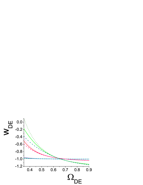
Figure 1: (Color online) A comparison between the exact result for $w_{DE}(\Omega_{DE})$ for $V_{\phi}(\phi)=\phi^{2}$, $V_{\sigma}(\sigma)=\sigma^{2}$ (dotted curves), the exact result for $w_{DE}(\Omega_{DE})$ for $V_{\phi}(\phi)=\phi^{-2}$, $V_{\sigma}(\sigma)=\sigma^{-2}$ (dashed curves), and our approximated analytical result for $w_{DE}(\Omega_{DE})$ provided by relation (33) (solid curves). The group of curves from top to bottom correspond to $\lambda_{0}=0.7$, $\theta_{0}=0.7$, to $\lambda_{0}=0.4$, $\theta_{0}=0.4$ and to $\lambda_{0}=0.1$, $\theta_{0}=0.4$. The error of our analytical result increases with the increase of $\lambda_{0}$ and $\theta_{0}$, and with the increase of the distance of $w_{DE}$ from $-1$.

From top to bottom the group of curves correspond to $\lambda_{0}=0.7$, $\theta_{0}=0.7$, to $\lambda_{0}=0.4$, $\theta_{0}=0.4$ and to $\lambda_{0}=0.1$, $\theta_{0}=0.4$. In addition, for the same parameter values we have used relation (33) to obtain the approximated analytical behavior (solid curves). As can be seen, the deviation from the exact solution is larger for larger distance of $w_{DE}$ from $-1$, which was expected since we have approximated $|1+w_{DE}|$ to be much smaller than $1$. Secondly, we observe that the error of our approximated result increases with the increase of the parameters $\lambda_{0}$ and $\theta_{0}$, i.e from bottom to top, which was also expected since we have assumed $|\lambda_{0}|,|\theta_{0}|\ll 1$. Thus, fig. 1 constraints the applicability range of our approximated analytical solution to $-1.1<w_{DE}<-0.9$ and $|\lambda_{0}|,|\theta_{0}|\lesssim 0.5$. We mention that for higher parameter values or for models with $w_{DE}$ larger than 0, the deviation of our approximated solution from the exact cosmological evolution can be dramatic, and our approximation scheme brakes down. But these cosmological scenarios are beyond the purpose of the present work. Finally, note that independently of the subsequent cosmological evolution, negative power-law potentials negpot can fulfill the nearly-flat potential conditions (29) if $\phi_{0}$ is sufficiently large. This feature shows that any potential can give rise to the type of models discussed here, as long us they satisfy (29), and this was also shown in Scherrer:2007pu for the case of thawing quintessence scenario.

Having determined the applicability area of our approximated scheme we proceed to specific cosmological scenarios. In fig. 2 we depict $w_{DE}(\Omega_{DE})$, given by (33), for five different models.

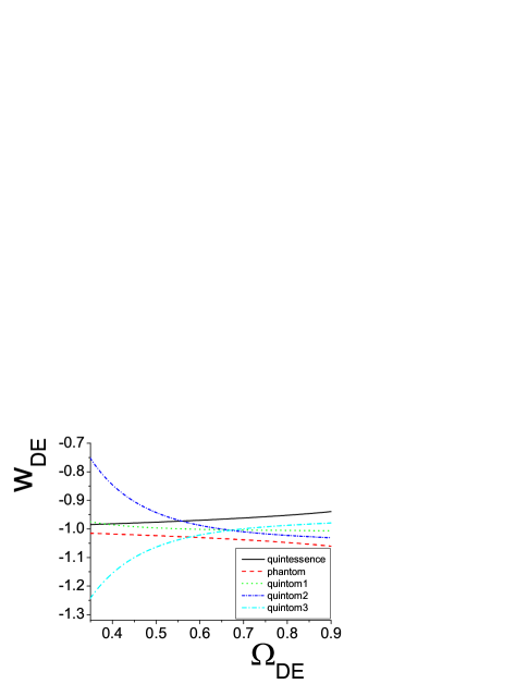
Figure 2: (Color online) $w_{DE}(\Omega_{DE})$ provided by relation (33) for various cosmological paradigms. The solid and the dashed curves correspond to simple quintessence and simple phantom models, with $\lambda_{0}^{2}=0.5$ and $\lambda_{0}^{2}=-0.5$ respectively. The dotted curve (quintom1) corresponds to $\lambda_{0}=0.1$, $\theta_{0}=0.4$. The sort-dashed-dotted curve (quintom2) corresponds to $\lambda_{0}=0.3$, $\theta_{0}=0.1$. The dashed-dotted curve (quintom3) corresponds to $\lambda_{0}=0.3i$, $\theta_{0}=0.1i$.

Firstly, with the solid and the dashed curves we present the simple quintessence and the simple phantom scenarios, that is when $\theta_{0}=0$ and $\lambda_{0}^{2}=0.5$, $\lambda_{0}^{2}=-0.5$ respectively. These results coincide with those of Scherrer:2007pu and Scherphan , noting that in these works the authors draw $w_{DE}(a)$ instead of $w_{DE}(z)$. As it was known, the simple quintessence and the simple phantom models cannot describe the transition through the phantom divide $-1$, and $w_{DE}$ remains always on the same side of this bound ($w_{DE}>-1$ for quintessence and $w_{DE}<-1$ for the phantom scenario). However, the combined consideration of both models can indeed describe the $-1$-crossing. In fig. 2 we depict $w_{DE}(\Omega_{DE})$ for three different quintom models. The dotted curve (quintom1) corresponds to $\lambda_{0}=0.1$, $\theta_{0}=0.4$, the sort-dashed-dotted curve (quintom2) corresponds to $\lambda_{0}=0.3$, $\theta_{0}=0.1$ and the dashed-dotted curve (quintom3) corresponds to $\lambda_{0}=0.3i$, $\theta_{0}=0.1i$. As we observe, all three models present the phantom-divide crossing.

In order to acquire a more transparent picture, in fig. 3 we depict $w_{DE}(z)$ (given by relation (35) with $\Omega_{DE_{0}}\approx 0.73$) for the same cosmological models of fig. 2.

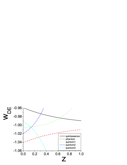
Figure 3: (Color online) $w_{DE}(z)$ provided by relation (35) with $\Omega_{DE_{0}}\approx 0.73$, for various cosmological paradigms. The solid and the dashed curves correspond to simple quintessence and simple phantom models, with $\lambda_{0}^{2}=0.5$ and $\lambda_{0}^{2}=-0.5$ respectively. The dotted curve (quintom1) corresponds to $\lambda_{0}=0.1$, $\theta_{0}=0.4$. The sort-dashed-dotted curve (quintom2) corresponds to $\lambda_{0}=0.3$, $\theta_{0}=0.1$. The dashed-dotted curve (quintom3) corresponds to $\lambda_{0}=0.3i$, $\theta_{0}=0.1i$.

As we observe, although all three examined quintom models can describe the phantom-divide crossing, only quirnom1 and quintom2 present the desired behavior, that is $w_{DE}(z)$ crossing $-1$ from above, resulting to $w_{{DE_{0}}}<-1$ at present, as it might be the case according to observations. We remind that according to (30) and (31), imaginary values correspond to initial phantom dominance, while real parameter values correspond to initial canonical-field dominance. Thus our framework reveals a way of determining the specific features of a quintom model. In particular, the crossing through $-1$ requires a sign change of $x^{2}$ (see relation (23)), and thus a change in which field’s kinetic term is larger (see definition (14)). If initially (with “initial” having the meaning of the beginning of slow-roll as considered in Scherrer:2007pu ; Scherphan ) is the canonical field that is dominant and at some point the phantom field dominates the evolution, then the crossing of $-1$ is from above to below. This case corresponds to quintom1 and quintom2 paradigms of fig. 3. On the other hand, if initially the evolution is dominated by the phantom field, and progressively by the canonical field, then the crossing through $-1$ takes place from below to above. This is the case of quintom3 scenario of fig. 3. Therefore, in order to describe the possible crossing of $w_{DE}(z)$ one has to consider an initial canonical field dominance, with a subsequent increase and dominance of the phantom field. These conditions are necessary for a certain $-1$-crossing, bur are not efficient. That is, if the initial dominance of one of the fields is sufficiently strong, then $w_{DE}(z)$, although moving towards $-1$, it will never succeed to cross it.

Let us close this section with a quantitative discussion. Current observations of $w_{DE}(z)$ 1 ; 2 ; 3 ; 4 can accept the description of quintom models with nearly flat potentials presented here. The most significant advantage of this scenario is the capability of describing the crossing through the phantom divide from above to below, in the near cosmological past, if such a crossing will be retained by future and more exact observations. In addition, even without a crossing, the model at hand can describe the $w_{DE}(z)$-evolution in close agreement with current observational limits. However, we mention that such a description is quantitatively trustworthy if the current value $w_{{DE_{0}}}$ is larger than $-1.1$ and smaller than $-0.9$. On the contrary, if $w_{{DE_{0}}}\lesssim-1.1$ or $w_{{DE_{0}}}\gtrsim-0.9$, then the errors of our approximated analytical solution (35) become relatively large and the results have to be considered only qualitatively.

IV Conclusions

In this work we examine quintom models with nearly flat potentials, without the assumption of complete dark energy domination. In the case where the dark energy equation-of-state parameter $w_{DE}$ is close to $-1$, we provide analytically an approximated universal expression for $w_{DE}(z)$ for all such models. This expression depends only on the initial conditions (beginning of slow roll), i.e on the values of the potentials and their derivatives at a specific point, and on the values of the field kinetic terms at the same point. This feature arises because, due to the potential flatness, the fields never roll very far along the potentials in order to “feel” the rest of their shape.

Contrary to the case of simple quintessence or simple phantom models, where $w_{DE}(z)$ is always on the same side of the phantom divide ($w_{DE}>-1$ for quintessence and $w_{DE}<-1$ for the phantom scenario) the quintom paradigm allows for a description of the transition through $-1$. In addition, we provide the necessary conditions for a specific such crossing. In particular, if initially the universe is dominated by the canonical field then the subsequent evolution can bring the phantom field domination and thus the $-1$-crossing from above to below. On the other hand, if initially is the phantom field that dominates then the evolution can lead to $-1$-crossing from below to above. Thus, a not-very-strong initial dominance of the canonical field can lead to a cosmological evolution where $w_{DE}(z)$ crosses $-1$ from above to below in the near past. In conclusion, the determination of the impact of the two fields, can provide a $w_{DE}(z)$-evolution in agreement with current observational limits.

Acknowledgements:

E. N. Saridakis wishes to thank Institut de Physique Théorique, CEA, for the hospitality during the preparation of the present work.

References

- (1) S. Perlmutter et al. [Supernova Cosmology Project Collaboration], Astrophys. J. 517, 565 (1999).
- (2) C. L. Bennett et al., Astrophys. J. Suppl. 148, 1 (2003).
- (3) M. Tegmark et al. [SDSS Collaboration], Phys. Rev. D 69, 103501 (2004).
- (4) S. W. Allen, et al., Mon. Not. Roy. Astron. Soc. 353, 457 (2004).
- (5) P. S. Apostolopoulos, and N. Tetradis, Phys. Rev. D 74, 064021 (2006); H.-S. Zhang, and Z.-H. Zhu, Phys. Rev. D 75, 023510 (2007).
- (6) S.Nojiri and S. D. Odintsov, Phys. Rev. D 68, 123512 (2003); P. S. Apostolopoulos, N. Brouzakis, E. N. Saridakis and N. Tetradis, Phys. Rev. D 72, 044013 (2005); S.Nojiri and S. D. Odintsov, Int. J. Geom. Meth. Mod. Phys. 4, 115 (2007); M. R. Setare and E. N. Saridakis, Phys. Lett. B 670, 1 (2008).
- (7) P. J. Peebles and B. Ratra, Rev. Mod. Phys. 75, 559 (2003); J. Kratochvil, A. Linde, E. V. Linder and M. Shmakova, JCAP 0407 001 (2004); F. K. Diakonos and E. N. Saridakis, [arXiv:0708.3143 [hep-th]].
- (8) R. R. Caldwell, R. Dave and P. J. Steinhardt, Phys. Rev. Lett. 80, 1582 (1998); M. S. Turner and M. White, Phys. Rev. D 56, 4439 (1997); T. Chiba, Phys. Rev. D 60, 083508 (1999); Z. K. Guo, N. Ohta and Y. Z. Zhang, Phys. Rev. D 72, 023504 (2005); Z. K. Guo, N. Ohta and Y. Z. Zhang, Mod. Phys. Lett. A 22, 883 (2007).
- (9) R. R. Caldwell, Phys. Lett. B 545, 23 (2002); S. Nojiri and S. D. Odintsov, Phys. Lett. B 562, 147 (2003); S. Nojiri and S. D. Odintsov, Phys. Rev. D 72, 023003 (2005); H. Garcia-Compean, G. Garcia-Jimenez, O. Obregon, and C. Ramirez, JCAP 0807, 016 (2008); M. Jamil, M. Ahmad Rashid, and A. Qadir, [arXiv:0808.1152 [astro-ph]].
- (10) R. R. Caldwell, M. Kamionkowski and N. N. Weinberg, Phys. Rev. Lett. 91, 071301 (2003).
- (11) Z. K. Guo, et al., Phys. Lett. B 608, 177 (2005); J.-Q. Xia, B. Feng and X. Zhang, Mod. Phys. Lett. A 20, 2409 (2005); M.-Z Li , B. Feng, X.-M Zhang, JCAP, 0512, 002, (2005); B. Feng, M. Li, Y.-S. Piao and X. Zhang, Phys. Lett. B 634, 101 (2006); M. R. Setare, Phys. Lett. B 641, 130 (2006); W. Zhao and Y. Zhang, Phys. Rev. D 73, 123509, (2006) ; G.-B. Zhao, J.-Q. Xia, B. Feng and X. Zhang, Int. J. Mod. Phys. D 16, 1229 (2007); M. R. Setare, J. Sadeghi, and A. R. Amani, Phys. Lett. B 660, 299 (2008); J. Sadeghi, M. R. Setare , A. Banijamali and F. Milani, Phys. Lett. B 662, 92 (2008); M. R. Setare and E. N. Saridakis, Phys. Lett. B 668, 177 (2008); M. R. Setare and E. N. Saridakis, [arXiv:0807.3807 [hep-th]]; M. R. Setare and E. N. Saridakis, JCAP 09, 026 (2008).
- (12) K. Griest, Phys. Rev. D66, 123501 (2002); S. Bludman, Phys. Rev. D69, 122002 (2004); R.R. Caldwell and E.V. Linder, Phys. Rev. Lett. 95, 141301 (2005); E.V. Linder, Phys. Rev. D73, 063010 (2006); S. Chongchitnan and G. Efstathiou, Phys. Rev. D76, 043508 (2007).
- (13) J. Kujat, R. J. Scherrer and A. A. Sen, Phys. Rev. D 74, 083501 (2006) [arXiv:astro-ph/0606735].
- (14) Q. G. Huang, Phys. Rev. D 77, 103518 (2008); E. N. Saridakis, [arXiv:0811.1333 [hep-th]].
- (15) R. J. Scherrer and A. A. Sen, Phys. Rev. D 77, 083515 (2008).
- (16) R. J. Scherrer and A. A. Sen, Phys. Rev. D 78, 067303 (2008).
- (17) E. J. Copeland, A. R. Liddle and D. Wands, Phys. Rev. D 57, 4686 (1998).
- (18) R. Crittenden, E. Majerotto and F. Piazza, Phys. Rev. Lett. 98, 251301 (2007).
- (19) M. Chevallier and D. Polarski, Int. J. Mod. Phys. D 10, 213 (2001); E.V. Linder, Phys. Rev. Lett. 90, 091301 (2003).
- (20) B. Ratra and P.J.E. Peebles, Phys. Rev. D37, 3406 (1988); R.R. Caldwell, R. Dave, and P.J. Steinhardt, Phys. Rev. Lett. 80, 1582 (1998).