Energy resolution and discretization artefacts in the numerical renormalization group
Abstract
We study the limits of the energy resolution that can be achieved in the calculations of spectral functions of quantum impurity models using the numerical renormalization group (NRG) technique with interleaving (-averaging). We show that overbroadening errors can be largely eliminated, that higher-moment spectral sum rules are satisfied to a good accuracy, and that positions, heights and widths of spectral features are well reproduced; the NRG approximates very well the spectral-weight distribution. We find, however, that the discretization of the conduction-band continuum nevertheless introduces artefacts. We present a new discretization scheme which removes the band-edge discretization artefacts of the conventional approach and significantly improves the convergence to the continuum () limit. Sample calculations of spectral functions with high energy resolution are presented. We follow in detail the emergence of the Kondo resonance in the Anderson impurity model as the electron-electron repulsion is increased, and the emergence of the phononic side peaks and the transition from the spin Kondo effect to the charge Kondo effect in the Anderson-Holstein impurity model as the electron-phonon coupling is increased. We also compute the spectral function of the Hubbard model within the dynamical mean-field theory (DMFT), confirming the presence of fine structure in the Hubbard bands.
pacs:
71.27.+a, 05.10.Cc, 72.10.Fk, 72.15.QmI Introduction
Condensed-matter systems often exhibit rather complex behavior due to strong Coulomb repulsion between the electrons at short distances. These effects become very pronounced when electrons are strongly confined either in inner electron shells (transition and rare-earth atoms) or in artificial nanostructures (quantum dots). Theoretical studies of the corresponding many-particle problems rely increasingly on advanced computational techniques such as the numerical renormalization group (NRG) Wilson (1975); Krishna-murthy et al. (1980a); Bulla et al. (2008). The NRG allows to study both static and dynamic Sakai et al. (1989); Sakai and Shimizu (1992); Costi et al. (1994); Bulla et al. (1998); Hofstetter (2000); Peters et al. (2006); Weichselbaum and von Delft (2007) properties of quantum impurity models like the Kondo model or the Anderson impurity model. Applications range from studies of thermodynamic properties of magnetic impurities in normal Krishna-murthy et al. (1980a, b); Oliveira and Wilkins (1981) and superconducting Satori et al. (1992); Sakai et al. (1993) host metals, dissipative two-state systems Costi and Kieffer (1996), electron transport through nanostructures Izumida et al. (1998), to the use of the NRG as an impurity solver in the dynamical mean-field theory (DMFT) Sakai and Kuramoto (1994); Bulla (1999); Pruschke et al. (2000); Georges et al. (1996).
The foundation of the NRG is the transformation of a model with an infinite number of degrees of freedom (the continuum of the conduction-band electron states) to a model with a finite number of lattice sites (known as the “hopping Hamiltonian” or the “Wilson chain”) which is numerically tractable using a computer. This transformation consists of three steps: 1) logarithmic discretization of the conduction band into increasingly narrow intervals around the Fermi level, 2) dismissal of combinations of states which do not couple directly to the impurity, and 3) unitary transformation to a basis in which the conduction-band Hamiltonian takes the form of a semi-infinite chain with exponentially decreasing hopping between neighboring sites. In the first step, the discretization is controlled by a parameter , which sets the energy widths of the intervals; the continuum is restored in the limit, while typical values used in practical calculations are or even much higher, depending on the application. The main approximation in the NRG intervenes in the second step (dismissal of higher modes); this approximation is controlled and it becomes better as is decreased Wilson (1975). An alternative discretization scheme Campo and Oliveira (2005) leads directly to the decoupling of higher modes at the price of using a non-orthogonal basis. The third step (mapping from the “star Hamiltonian” to a “chain Hamiltonian”) can, in fact, be omitted Bulla et al. (2005) at the cost of significantly higher computational requirements.
After these initial steps, the Hamiltonian is diagonalized iteratively, taking one more chain site into account in each NRG iteration. Since the Hilbert space grows exponentially, only a finite number of low-lying states are kept in each iteration, while high-energy states are discarded (truncated). This procedure is possible due to the “separation of energy scales” which simply means that the matrix elements between the bottom and top end of the excitation spectrum are small Wilson (1975); this is an important property of quantum impurity models. Truncation is another source of systematic errors in NRG. These errors are more difficult to estimate a-priori, but they can be kept small by a proper choice of and by performing the truncation at suitably high cutoff energy.
While the NRG is the method of choice to study low-energy properties of quantum impurity models, it is, however, commonly believed that it has inherently limited energy resolution at higher energies due to the discretization of the conduction band. This is particularly relevant for the calculations of dynamic properties Sakai et al. (1989); Sakai and Shimizu (1992); Costi et al. (1994), such as the impurity spectral function or the dynamical susceptibilities. Since the continuum impurity model is mapped onto a finite chain, the spectral function consists of a set of delta peaks with given energies and weights. These peaks need to be broadened Costi et al. (1994); Bulla et al. (2001, 2008) to obtain the desired final result: a smooth spectral density function. In order to efficiently smooth out spurious oscillations, broadening kernel functions with long tails are usually chosen. The log-Gaussian broadening function is very commonly used since it is well adapted to the logarithmic discretization grid. Unfortunately, the slowly decaying tails lead to strong overbroadening effects, restraining the effective energy resolution at higher energies and completely washing out any narrow spectral features with small spectral weight.
Narrower broadening functions can be used when the so-called interleaved method (also known as the “-averaging”) is used Oliveira and Oliveira (1994); Silva et al. (1996); Paula et al. (1999); Campo and Oliveira (2005). The interleaved method consists of performing several NRG calculations for different (interleaved) logarithmic discretization meshes controlled by the “twist” parameter . In this way, the information is sampled from different energy regions in each NRG run. The spectral function is then computed by averaging over all values. Although the interleaved method does not truly restore the continuum limit, it is surprisingly successful in removing oscillatory features in the spectra; even averaging over only two values of is often very beneficial.
In this work, we study to what extent the energy resolution of the NRG can be ultimately improved by the interleaved method. We perform the averaging over a very large number of values of and use very narrow Gaussian broadening kernel of width proportional to the energy of each individual delta peak. This approach, although rather costly in terms of the required computational resources, eliminates overbroadening and provides spectral functions with very high energy resolution even on the energy scale of the width of the conduction band. In addition to allowing us to study the fine structure in the spectral functions of impurity models, this high-resolution approach also uncovers the artefacts which are inherent in the NRG and cannot be eliminated by the -averaging. The artefacts diminish as is decreased, but they are present in any practical NRG calculation. By determining the appearance of the artefacts and their expected locations, one can properly take them into account when interpreting the results. We also propose a new discretization procedure which is very successful in removing the most severe NRG discretization artefacts. This improvement makes NRG a powerful technique for accurately studying both low and high energy scales, thereby increasing its value as a reliable impurity solver in DMFT.
This work is structured as follows. We introduce the Anderson impurity model in Sec. II and the details of the NRG calculations in Sec. III. To explore how accurately NRG approximates the spectral-weight distribution, we present in Sec. IV the sum rules for spectral functions of the Anderson impurity model, the fulfilment of which is then studied in Sec. V. The discretization artefacts are discussed in Sec. VI, while in Sec. VII, we present the modification to the discretization scheme which renders these artefacts less severe. In Sec. VIII we present examples of high-resolution spectral functions for the Anderson and Anderson-Holstein impurity models which reveal interesting details, which cannot be easily obtained by any other method. Finally, in Sec. IX we demonstrate the feasibility of using the high-resolution NRG approach in a DMFT setup. The resolution is sufficient to resolve the fine structure in the Hubbard bands, in particular the accumulation of the spectral weight at inner Hubbard band edges.
II Anderson impurity model
We consider the Anderson impurity model Anderson (1961), the paradigm of the quantum impurity models. It is defined by the following Hamiltonian
| (1) |
where operators describe the continuum conduction-band electrons and operators the impurity level, is the band dispersion, the impurity hybridisation, the number of the lattice sites, the impurity energy and the on-site electron-electron repulsion. Furthermore, and . In the derivations to follow, it is more convenient to rewrite the hybridisation part of the Hamiltonian as Wilson (1975)
| (2) |
Here the hybridisation constant is defined as
| (3) |
and the operator as
| (4) |
The operator thus describes the combination of band states which couple directly to the impurity level. The hybridisation strength is given by , where is the density of states (DOS) in the conduction band. In numerical calculations we will use a constant DOS , where is the bandwidth, unless noted otherwise.
In the NRG, the continuum of band electrons is reduced to the hopping Hamiltonian
| (5) |
The operator represents the previously introduced combination of states, while for describe further orbitals along the Wilson chain. The coefficients depend on the discretization scheme and on the parameters and ; asymptotically they behave as . We emphasize that this is not an exact representation of the continuum band Hamiltonian.
III Method
Dynamical NRG calculations were performed using the density-matrix approach Hofstetter (2000); Žitko and Bonča (2006a); Tóth et al. (2008) using the density matrix computed at the energy scale of . Spectral functions were obtained by delta-peak broadening using a Gaussian kernel with a width proportional to the peak energy Sakai et al. (1989); Costi and Hewson (1992):
| (6) |
where is the energy of the point in the spectrum, is the delta-peak energy and the width of the Gaussian is with a constant (we mostly use or ); the relative spectral resolution is thus expected to be constant, . For the purposes of obtaining high-resolution spectral functions, it is very important to use Gaussian broadening rather than, for example, Lorentzian broadening, due to the fast decrease to zero of the Gaussian function. We also note that the conventional log-Gaussian broadening kernel becomes equivalent to a simple Gaussian kernel for small enough , aside from a small asymmetry of the log-Gaussian function. Furthermore, parameters and are related by in this limit. Nevertheless, the symmetry of the Gaussian function is beneficial for the purposes of this work. For some further comments on the spectral function broadening, see Appendix A.
The discretization was performed using the non-orthogonal-basis-set approach of Campo and Oliveira Campo and Oliveira (2005), with averaging over or values of the twist parameter , equally distributed in the interval . We note that in order to obtain a smooth spectrum, and need to be chosen such that is of order 1.
The truncations were performed at an energy cutoff , where is the characteristic energy scale at the -th NRG iteration. When necessary, additional states were retained above this cutoff energy to ensure that the truncation was performed within an energy “gap” of at least , so as not to introduce systematic errors which may arise by retaining only parts of clusters of nearly degenerate states. Charge conservation and spin invariance have been explicitly taken into account.
Spectral functions were obtained by “patching” together spectral functions from every second energy shell (the approach) Bulla et al. (2001). The details of the patching approach are important and, if not done properly, the procedure will accentuate the discretization artefacts. At every even- NRG interaction, we perform the patching as described in Ref. Bulla et al., 2001: we merge spectral peaks in the energy range (unmodified) and spectral peaks in the range (after linear rescaling) with the total spectral density; is some constant that we refer to as the “patching parameter”. We return to the patching procedure in Sec. VI, where we also comment on the relative merits of the patching approach and the complete-Fock-space technique Peters et al. (2006); Weichselbaum and von Delft (2007).
IV Higher-moment spectral sum rules for the Anderson impurity model
A simple way of quantifying the distribution of the spectral weight is through the moments, defined as
| (7) |
where is the spectral function. A stringent test of the calculated dynamic property (spectral function) is to verify that it satisfies the sum rules which relate the moments to various static quantities (expectation values). The zero-th moment is simply the normalization condition for spectral functions
| (8) |
Higher-moment spectral sum rules for the Anderson impurity model can be derived as Bulla et al. (2008); White (1991)
| (9) |
where is the iterated commutator, defined recursively as
| (10) |
while is the anticommutator. The first moment (mean energy) is simply the Hartree energy of the impurity level,
| (11) |
while the second is
| (12) |
The variance of the spectral function is thus
| (13) |
i.e. a sum of the hybridisation width and the interaction-induced width. The third moment is
| (14) |
Here the operator is the -orbital occupancy and the operators are hopping operators between the impurity orbital and the site of the Wilson chain. The third central moment is thus
| (15) |
which simplifies in the non-interacting limit to .
The fourth moment is
| (16) |
where operator ; here is the two-particle hopping operator and is the transverse part of the spin-exchange operator. In the non-interacting limit, the fourth moment simplifies to
| (17) |
It is important to point out that the expressions for and depend on the discretization through the coefficient and the operator (for this is the case only for ). They are therefore not exact. While it is possible to derive exact expressions in terms of , and operators , they are of little practical use. This implies that in the interacting case, calculations of and and the fulfilment of the corresponding sum rules must be considered above all as a test of the internal consistency of the method and of the extent of errors brought about by the NRG truncation (“energetics”). Comparison with exact and (were they known) would inevitably show some discrepancy (in the following, we will demonstrate such behavior for in the non-interacting case).
V Spectral weight distribution and sum rules
V.1 Non-interacting case
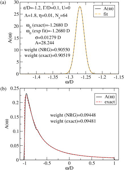
We first consider the non-interacting () resonant-level model. The spectral moments are tabulated in Table 1. The spectral function of this model is given exactly as
| (18) |
with
| (19) |
for . This expression for is used to compute the reference values for spectral moments exactly (second column, ). The right-hand sides of the sum rules, Eq. (9), are computed in the standard way with (third column, ) Wilson (1975); Krishna-murthy et al. (1980a); Bulla et al. (2008). The fourth column contains moments calculated by summing the suitably weighted delta-peak contributions to the spectral function, , and finally the fifth column contains moments calculated directly by performing a numerical integration with a spectral function after broadening, .
| Moment | Exact, | Static, | Dynamic (delta peaks), | Dynamic (broadened), |
|---|---|---|---|---|
| 1 | 0.999442 | 0.999981 | ||
| -0.050000 | -0.050000 | -0.049983 | -0.049999 | |
| 0.0056831 | 0.0056831 | 0.0056866 | 0.0056871 | |
| -0.00044331 | -0.00044331 | -0.00044366 | -0.00044389 | |
| 0.00110129 | 0.0010225 | 0.0010220 | 0.0010225 |
The first three moments calculated as static quantities, , trivially agree with exact values since they are constants, while there is a 7 percent discrepancy for the fourth. This can be attributed to the discretization errors as described previously in Sec. IV. It must be noted, however, that the fourth moment of a Lorentzian peak located near the Fermi level strongly depends on the details around the band edges and contains little information about the spectral distribution in the frequency range of interest (i.e. around the peak itself). More importantly, we find good agreement between and the moments computed from dynamic quantities, and , with errors in the few permil range. This internal self-consistency of the method implies that the accuracy of the energy levels in the range where the contributions to the spectral function are sampled from is very good. The difference between results from a calculation from delta-peak weights, , or from broadened spectral function, , is remarkably small. This already suggest that the broadening procedure itself does not lead to any appreciable overbroadening.
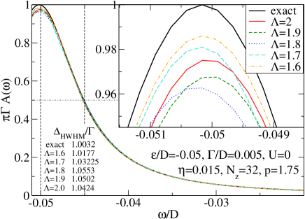
To study how the logarithmic discretization affects the spectral weight distribution, we plot the spectral function of the non-interacting model for a range of values of the discretization parameter , Fig. 1. The peak position, width and height are well reproduced; the position to within less than one percent even at , while the height and the half-width at half-maximum both deviate by less than 5 percent. As expected, the agreement improves as is decreased, although not in a uniform manner. It may be noted that some spectral weight seems to be missing in the peak (with the situation improving as ). This is indeed the case; the missing spectral weight is located in the NRG discretization artefacts that are the topic of Sec. VI.
V.2 Interacting case
We now switch on the interaction and consider an asymmetric Anderson impurity model in the Kondo regime, . Exact results for moments are not available in this case, but we can compare and , Table 2. We find a similar degree of agreement (few permil) as in the non-interacting case. We also observe that the moments (and ) calculated for each value of separately depend relatively little on . This is somewhat surprising given that unaveraged spectral functions are extremely oscillatory. It also implies that if we are really interested in a quantity which can be expressed as an integral of the spectral function multiplied by some relatively smooth weight function, there is only little benefit in performing the -averaging.
| Moment | Static, | Dynamic (delta peaks), | Dynamic (broadened), |
|---|---|---|---|
| 1.000303 | 1.000306 | ||
| -0.0123204 | -0.0123184 | -0.0123184 | |
| 0.00455271 | 0.00455556 | 0.00455549 | |
| -0.000138146 | -0.000138222 | -0.0001381970 | |
| 0.0010179 | 0.00101737 | 0.00101748 |
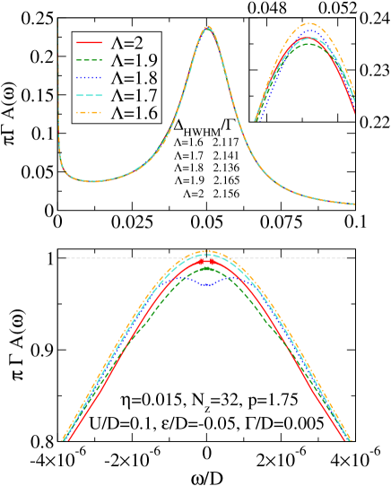
We now study the spectral function of the symmetric Anderson impurity model shown for a range of discretization parameters in Fig. 2. The spectral functions overlap to a very good approximation and there is little systematic overbroadening. The width of the charge-transfer peak is, as expected, approximately . The Kondo resonance is well reproduced with a notable exception of , where we find an artefact which takes the form of a depression at the top of the Kondo resonance. For this value of , the Friedel sum rule is strongly violated. This is another manifestation of the NRG artefacts that will be discussed in the following; the result is improved by tuning the patching parameter .
A very successful method to reduce overbroadening effects in NRG calculations is the “self-energy trick” Bulla et al. (1998). It consists of numerically computing the self-energy as the ratio where and and then computing an improved Green’s function as
| (20) |
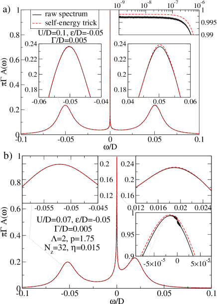
An additional merit of this technique is that it leads to a partial cancellation of the oscillatory features in and , giving a smooth self-energy . In Fig. 3 we compare raw and self-energy-improved spectral functions for the symmetric and asymmetric Anderson model. We first note that the change of the spectral function upon using the self-energy trick is rather small, unlike in the case of log-Gaussian broadening with large where the self-energy trick leads to a sizable improvement and reduction of overbroadening. Results for the symmetric case (Fig. 3a) show that while the Friedel sum rule is satisfied to better accuracy, the self-energy trick leads to slightly broken particle-hole symmetry in the final result, which is not desirable. On the other hand, in the general asymmetric case the self-energy trick cures problems associated with different limiting behavior of for and , respectively (see Fig. 3b, inset with the close-up on the Kondo resonance).
VI Discretization artefacts
VI.1 Types of artefacts
Closer inspection of the computed high-resolution spectral functions reveals the presence of artefacts which cannot be entirely eliminated by increasing or reducing . These are thus genuine intrinsic NRG discretization artefacts.
As a first example, we plot in Fig. 4a the spectral function of the non-interacting impurity model in the high-energy range near the band edge, i.e. the tail of the Lorentzian spectral peak. We see a pronounced artefact which shifts toward the band-edge as is decreased. If the exact solution is subtracted from the artefact, we find that there is some cancellation of positive and negative differences, but there is nevertheless a positive net (integrated) difference; this is the origin of the previously mentioned missing spectral weight in the spectral peak of the resonant-level model. In the inset we show the spectral function of the first site of the Wilson chain . For a flat band, , this function should likewise be flat, except for the features that are mirrored from the impurity spectral function . The NRG discretization, however, introduces additional artefact structure for energies near the band-edge.
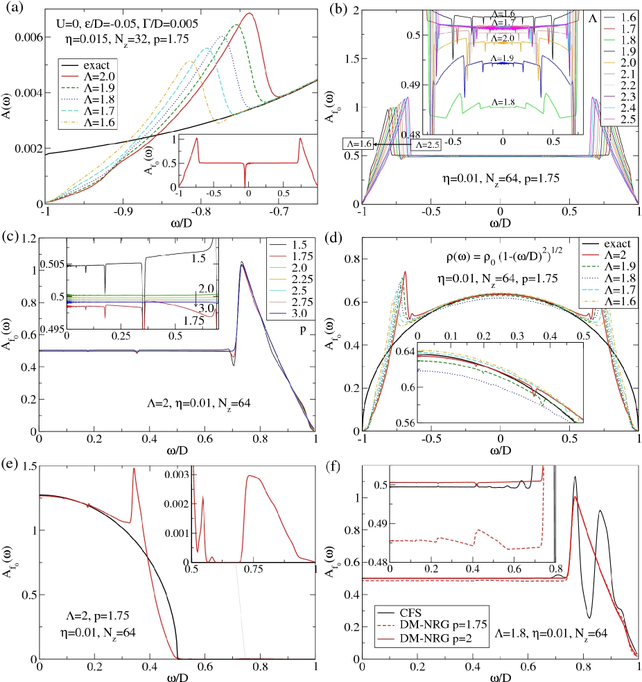
To study this problem more closely, we compute for a system without the impurity, Fig. 4b. In addition to the very pronounced band-edge artefact, there are also discernible additional artefacts at lower energies. The ratio of energies for two consecutive artefacts is , as expected. The artefact peaks presumably exist down to lowest energy scales, but their amplitudes decrease rapidly and eventually the peaks can no longer be resolved since they are masked by the residual oscillations in the calculated spectral functions. Curiously, the average value of in the low-energy region seems to have a minimum for . Furthermore, for this value of , the artefacts appear to be the largest. This is in agreement with the results for spectral functions presented above. These artefacts can, however, be strongly reduced finding proper parameter of the spectrum patching procedure.
In Fig. 4c we plot the spectral density for different values of . If is too small, we obtain very pronounced discretization artefacts. If is too large, the spectral density is underestimated. The optimal value of is around , but it depends on the energy cutoff in the truncation; we work with cutoff , thus for and , we have . We remark that the large artefacts near the band-edge are not related to the patching procedure (see also below), although the form of the artefacts does depend somewhat on the value of .
We can formulate the following recipe for choosing appropriate NRG parameters:
-
1.
fix ;
-
2.
increase truncation cutoff until NRG results no longer change significantly;
-
3.
tune and to suppress overbroadening of spectral functions;
-
4.
tune for good reproduction of the band spectral function .
If necessary, steps 2-4 may be reiterated. To be specific, for , , , and , we find that is closest to at low energies for . A caveat is in order: tuning for good reproduction of does not necessarily imply that the same value of will be optimal for the full problem (with the impurity coupled to the bath). Nevertheless, such is most likely a good choice.
For applications of the NRG as an impurity solver in DMFT, it is important to reproduce an arbitrary conduction-band DOS as accurately as possible. As a simple test, in Fig. 4d we consider the case of the cosine band dispersion, , which has a semi-elliptic DOS,
| (21) |
We again find sizable artefacts near band edges at approximately the same positions as in the case of a flat band. One might expect that using a DOS with a limited support (such that it excludes the strong artefacts at ) would resolve the issue. Alas, that is not the case. The artefacts simply appear at rescaled positions, as is shown in the example of a semi-elliptic DOS with support , Fig. 4e. Any abrupt change in the density of states (any sharp feature, in fact) is thus expected to lead to anomalies at low energies.
Spectra calculated using the complete-Fock-space (CFS) approach Peters et al. (2006); Weichselbaum and von Delft (2007) also show artefacts, although there are differences in the details, see Fig. 4f. There are several advantages to the CFS approach: the normalization is satisfied exactly within numerical accuracy and there is no ambiguity in the choice of the energy range where the spectrum is computed at each iteration (no parameter ). The conventional approach is, however, significantly faster since the eigenvectors and matrix elements need to be computed only in the retained part of the Hilbert space in each NRG iteration. In addition, in CFS the delta-peak energies are given as a difference between an energy of a kept state and an energy of a discarded state; the latter is located at the upper end of the shell excitation spectrum, thus it is affected by the accumulated truncation errors from all previous NRG iterations. For this reason, the spectra calculated using the traditional approach with patching satisfy higher-moment sum rules to higher accuracy (in the permil range as opposed to the percent range) even though they break the normalization sum rule.
VI.2 Origin of the band-edge artefacts
In the case of a flat band, , the origin of the main artefact near the band edge is easy to understand. Following Ref. Campo and Oliveira, 2005, we write the density of states on site as
| (22) |
where define the discretization mesh,
| (23) |
and are defined as
| (24) |
with , which gives
| (25) |
For given argument , the parameters and in the right hand side of Eq. (22) are determined by the relation which has a unique solution. (To simplify the notation and discussion, we assumed particle-hole symmetry of the conduction band and we consider only. All features at positive energies are then simply mirrored to negative frequencies.) It can be easily shown that for , i.e. for
| (26) |
we indeed have
| (27) |
This is not the case, however, for , i.e. for within from the band edges. We obtain, instead,
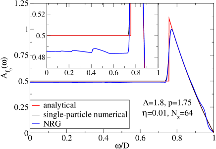
| (28) |
with , where is the Lambert W-function. In Fig. 5 we plot three spectral functions: 1) analytically calculated spectral function, , 2) the spectral function numerically calculated by exact diagonalisations of the single-electron Hamiltonians obtained after discretization, , and 3) the spectral function calculated directly using NRG, . Compared to the analytical result, , the function features artefacts due to finite and broadening, while in addition shows truncation errors. The band-edge artefact is thus not some unexpected numerical artefact, but it is the direct result of a particular choice of the discretization scheme. It arises from a different behavior of as a function of as compared to other . This, in turn, is due to the presence of the band-edge, which sets the upper boundary in the integrals in Eq. (24).
For arbitrary density of states we introduce weight functions for different discretization intervals Campo and Oliveira (2005)
| (29) |
so that the operator takes the following form
| (30) |
where are conduction-band operators for the -th mode (combination of states) in the -th discretization interval; only modes are retained in the NRG. The spectral function on the first site of the Wilson chain is then given as
| (31) |
where and are again determined by the relation . In order to achieve decoupling of higher modes in each discretization interval, Campo and Oliveira proposed to calculate coefficients as Campo and Oliveira (2005)
| (32) |
In the most commonly used conventional discretization scheme Yoshida et al. (1990), the coefficients are given, instead, as
| (33) |
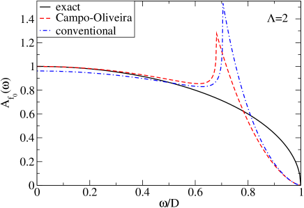
It is easy to verify that calculated in either way do not satisfy the equation and that strong artefacts appear near sharp features in the density of states. As an example, we compare in Fig. 6 the cosine band DOS with computed with both discretization schemes. Both show significant band-edge artefacts (see also Fig. 4d). In the conventional scheme, the spectral function in addition systematically underestimates at lower energy scales by the well-known factor of
| (34) |
which is taken into account in practical NRG calculations in an ad-hoc manner by multiplying the impurity hybridisation (or exchange constant) by this same value.
VII Overcoming the discretization artefacts
We have demonstrated that the origin of the discretization artefacts is in the -dependence of the coefficients . These coefficients, in turn, are determined by the discretization points , the choice of the basis states of the discretized conduction band (in particular the weight functions ) and the recipe for the calculation of coefficients Yoshida et al. (1990); Campo and Oliveira (2005). Keeping the same set of the discretization points and zero-mode basis states, we may decide to define in a more appropriate way, i.e. such that all coefficients satisfy the condition
| (35) |
Details about solving this equation are given in the Appendix B. Well-behaved solution may be found for arbitrary DOS function and the asymptotic (large ) behavior of is the same as in the Campo-Oliveira discretization scheme.
We note that this modification of the discretization procedure in no way makes NRG an exact method, even though we expect much better reproduction of the conduction band DOS. In the spirit of the original NRG procedure, we still rely on the assumption that discarding higher-mode states in each discretization interval is a good approximation which can be systematically improved by reducing toward 1. In particular, discretization-related artefacts are still possible and we indeed find them, as detailed in the following. The improvement consists in significantly reducing the severity of the artefacts.
Solving Eq. (35) in the case of a flat band, only is modified, while for remain the same. We obtain
| (36) |
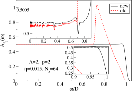
As is swept from 0 to 1, this quantity takes values over the same interval as the Campo-Oliveira expression for . This is important, since must cover the whole energy range. In Fig. 7 we compare the spectral function computed with original and modified discretization approach. The improvement is, as expected, significant. The spectral function overshoots slightly (by less than two percent) as the band-edge is approached and it decays to zero on the scale set by the broadening parameter . A closer look reveals small residual artefacts positioned at energies , , which take the form of asymmetric dips. Their weights rapidly decreases with increasing ; in the worst case, for , the dip amplitude is less than one permil of the background weight. There are further artefacts between the dips, but their amplitudes are even smaller than those of the main artefacts. At low energies, converges to , which can be tuned exactly to by further tuning of the patching parameter .
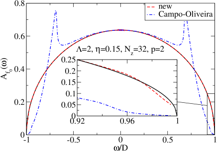
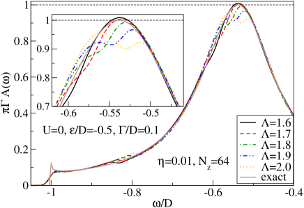
In Fig. 8 we compare the spectral functions of the resonant-level model obtained using both discretization schemes. We find that the new discretization scheme strongly suppresses the artefact peak structure and correctly reproduces the behavior at the very edge of the conduction band (within the limits imposed by the broadening procedure). We also see that the flanks of the spectral peak agree better with the exact solution. On the other hand, we see that an artefact appears at the very top of the resonance. This artefact is directly connected with the discretization itself and does not depend, for example, on the truncation or patching; the situation improves, however, with decreasing (see Fig. 12 in Subsection B below). We point out that the artefact is not located at any , thus it is not related to the residual artefacts found in of the decoupled band. It should rather be interpreted as a finite-size effect due to representation of the continuum by a finite chain; the -averaging cannot entirely eliminate such effects. In spite of the artefact, we may conclude that the overall reproduction of the spectral weight distribution is considerably improved. It may also be noted that we present here the most difficult case: a very broad resonance near the band edge. Such situation is rather unusual for impurity problems; for narrow resonances and for peak energies closer to the Fermi level the double-peak artefact is quickly reduced. Broad spectral distributions are, however, typical for DMFT applications, where residual artefacts may become more problematic.
In Tables 3 and 4 we show the moments for the non-interacting model and for the asymmetric Anderson model. They are to be compared with the corresponding Tables 1 and 2. The agreement between and in the new scheme is below one permil for all moments, as in the old one. In the resonant-level model, the agreement of calculated now agrees with the exact value within one permil (while in the Campo-Oliveira scheme we found a discrepancy of ). In the Anderson model, we also observe a change in of the same order, suggesting a similar degree of improvement.
| Moment | Exact, | Static, | Dynamic (delta peaks), | Dynamic (broadened), |
|---|---|---|---|---|
| 1 | 0.999979 | 0.999964 | ||
| -0.050000 | -0.050000 | -0.049998 | -0.049997 | |
| 0.0056831 | 0.0056831 | 0.0056876 | 0.0056704 | |
| -0.00044331 | -0.00044331 | -0.00044376 | -0.00044217 | |
| 0.00110129 | 0.00110120 | 0.00110158 | 0.0010842 |
| Moment | Static, | Dynamic (delta peaks), | Dynamic (broadened), |
|---|---|---|---|
| 1.000302 | 1.000287 | ||
| -0.0123213 | -0.0123193 | -0.0123187 | |
| 0.00455274 | 0.00455661 | 0.0045386 | |
| -0.000138138 | -0.000138191 | -0.000137434 | |
| 0.00109664 | 0.00109694 | 0.00107882 |
VII.1 Arbitrary density of states
In Fig. 9 we demonstrate on the example of the semi-elliptic DOS that the proposed discretization approach can also be applied for an arbitrary density of states. In this case, all are modified and they need to be numerically calculated using the technique described in the Appendix B. As in the case of flat band, some small discrepancies between and are found at the very edge of the band. The over-all agreement is, however, significantly improved on all energy scales.
We test the method on the case of a symmetric Anderson model with semi-elliptic DOS. In Fig. 10 we plot spectral functions for rather large for increasing values of . While for small the functions are rather smooth, we observe more pronounced residual artefacts for large values of , as the charge-transfer (Hubbard) peaks approach the band edge (see, for example, the case). Nevertheless, the results are significantly more physically sensible than those obtained using conventional broadening and discretization techniques. For , the Hubbard peaks are located outside the conduction band. They become narrower and they have strongly asymmetric shape Raas and Uhrig (2005); in fact, in some parameter ranges they have a two-peak structure. We also note that the impurity parameters used here are comparable to those that typically arise in effective models in DMFT (see also Sec. IX).
VII.2 Convergence with
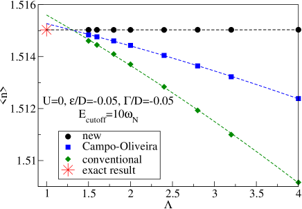
The new discretization scheme vastly improves the convergence to the limit. We demonstrate this in Fig. 11 by comparing the calculated level occupancy in the resonant-level model with the exact value as a function of . With the new approach, we obtain very accurate results even with very large discretization parameter (four digits of accuracy at ). In other approaches, not only is the convergence to the continuum limit slower, but extrapolating the numeric results in the range to the limit leads to a systematic error; presumably the assumption of quadratic (or polynomial) -dependence no longer holds for smaller . With the improved discretization approach one can compute expectation values of various operators reliably even at very large : this is quite important for numerically demanding multi-orbital/multi-channel quantum impurity problems. Similar improvements also hold for calculations of thermodynamic quantities (such as the impurity contribution to the magnetic susceptibility and entropy).
We have seen previously that residual artefacts are observed in spectral functions. In Fig. 12 we report how these residual artefacts are reduced as is reduced. For sufficiently small , the artefact appearing as double peak structure is eliminated. Furthermore, we see that the artefacts shift as a function of . This implies that some additional improvement could be obtained by performing the calculation for several different values of and averaging the resulting spectral functions.
In the sense that the new discretization scheme gives the best possible representation of the conduction band DOS by the Wilson chain (after the -averaging), this technique provides the best results that one can achieve by representing each discretization interval by a single level. A possible systematic improvement would consist in including more than one mode for low (where the band DOS still varies strongly as a function of energy) and performing the NRG in the star basis, perhaps using Lanczos exact diagonalisation procedure to diagonalize the cluster at each NRG iteration.
VII.3 Spectral features outside the conduction band
We tested how accurately the NRG reproduces spectral features at energies outside the energy band (i.e. outside the interval in the case of a flat conduction band) for the example of the resonant-level model. In this model, for , there is a -peak at the energy given by
| (37) |
with weight
| (38) |
while the spectrum in the range is described by Eq. (18). We compare the calculated spectrum with the expected results in Fig. 13. The -peak takes the form of the broadening kernel, Eq. (6), and we can accurately extract its position, height and width by fitting to an exponential function . We find that the position and the (integrated) weight of the peak are reproduced within approximately four digits of precision. Furthermore, we find that
| (39) |
which is to be compared with the broadening factor . We conclude that within one percent accuracy, there is no other source of broadening than the explicit spectral function broadening by the Gaussian broadening kernel. The agreement of the calculated spectral function within the conduction band, i.e. in the interval, Fig. 13b, with the exact result is also very satisfactory.
VIII High-resolution spectral functions
We present two examples of high-resolution calculations unmasking interesting details. We first study the emergence of the Kondo resonance as the electron-electron repulsion is increased in the Anderson impurity model. We then consider the Anderson-Holstein model to show that the phononic side peaks can be well resolved.
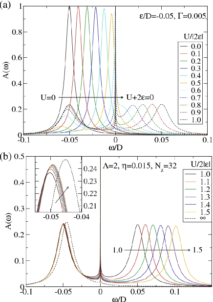
VIII.1 The emergence and the shape of the Kondo resonance
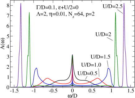
In Fig. 14 we show spectral functions for the Anderson impurity model for a range of values of the electron-electron interaction , from the non-interacting case to the symmetric situation (Fig. 14a) and then to the large- limit (Fig. 14b). Since these results are hardly affected by overbroadening, we can accurately follow the evolution of the spectral peak, its location as well as its height and width. In the non-interacting limit, the peak height is , its width is and it is centered at . As increases, the peak position shifts linearly with (Hartree shift), while its height decreases. The remaining spectral weight is located in the emerging lower charge-transfer spectral peak (i.e. the lower “Hubbard band”); this peak is initially located below , but it shifts to as we approach the particle-hole symmetric situation. The width of the charge-transfer peaks is roughly twice () the width of the original non-interacting peak (). As we increase further, Fig. 14b, the lower charge-transfer peak shifts only weakly as a function of , while the upper charge-transfer peak shifts as ; in the range of finite shown, its height decreases only slightly and the width remains nearly constant. At the same time, the width of the Kondo resonance is significantly reduced, but we find that it remains almost pinned at the Fermi level (at , for example, the half-width at half-maximum of the Kondo peak is , while the shift of the maximum is only , i.e. 3 percent in the units of HWHM). This is in agreement with the Fermi liquid theory, but in disagreement with the results from methods based on the large- expansion, such as the non-crossing approximation, which overestimate the shift of the resonance, in particular for . It also implies that the Kondo temperature should better not be defined as the displacement of the Kondo resonance from the Fermi level, as it is sometimes done.
In Fig. 15a we plot a close-up on the Kondo resonance in the symmetric case, . As expected, the peak shape deviates significantly from a Lorentzian shape Bulla et al. (2000); Dickens and Logan (2001); Glossop and Logan (2002); Rosch et al. (2003). In fact, true agreement is only found in the asymptotic region, where both the Lorentzian curve and the spectral function have quadratic frequency dependence. In the latter case, this is mandated by the Fermi-liquid behavior at low energy scales.
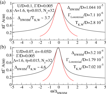
The relation between the width of the Kondo resonance and the Kondo temperature (times ) is of considerable experimental interest, in particular for tunneling spectroscopy. In the symmetric case, we find for the ratio between the half-width at half-maximum and the Kondo temperature (Wilson’s definition):
| (40) |
The Kondo temperature is defined as , where is Wilson number, and extracted from the NRG results for the magnetic susceptibility using the prescription . The same value of 3.7 is also obtained when log-Gaussian broadening is used with a small value of the parameter and with suitable -averaging. This ratio is lower than some other values reported in the literature Micklitz et al. (2006).
In Fig. 15b we plot the Kondo resonance in the asymmetric case. We find that the ratio between the half-width and the Kondo temperature is now . Even though we are still deep in the Kondo regime (phase shift is ), the Kondo peak has developed a significant asymmetry in its shape. These line-shape effects are important in the interpretation of experimental results. Due to uncertainties in the ratio , the expected systematic error in determining from the Kondo peak width is estimated to be several 10 percents. This implies that comparisons of of different adsorbate/surface systems determined in this way are rather meaningless unless the differences are of the order of a factor 2 or more.
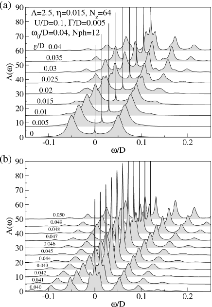
VIII.2 The phononic side-peaks in the Anderson-Holstein model
We consider the Anderson-Holstein model with coupling of a local Einstein phonon mode to charge fluctuations:
| (41) |
Here is the bosonic phonon operator, is the oscillator frequency and the coupling between the impurity charge and the oscillator displacement. This model was studied intensely using a variety of techniques, including NRG Hewson and Meyer (2002); Jeon et al. (2003); Cornaglia et al. (2004, 2005); Žitko and Bonča (2006b). Its applications range from the problem of small polaron and bipolaron formation, electron-phonon coupling in heavy fermions and valence fluctuation systems, to describing the electron transport through deformable molecules.
The effect of the electron-phonon coupling is to reduce the effective electron-electron interaction and shift the level energy Mahan (2000); Hewson and Meyer (2002):
| (42) |
In addition, the effective hybridisation becomes phonon-dependent, since the phonon cloud can be created or absorbed when the impurity occupancy changes Hewson and Meyer (2002).
It is possible to resolve the phononic side-peaks and the transition to the charge Kondo regime, Fig. 16. For small coupling , we see the gradual emergence of the phononic side-peaks at energies , . In addition to these peaks, we see that the charge transfer peak at itself has internal structure; as increases, part of the spectral weight is transferred from this peak to higher energies in the form of a smaller peak which eventually merges with the first phononic side-peak at . The transition from spin to charge Kondo regime occurs at , when . At the transition, the charge transfer peak merges with what used to be the Kondo resonance to give a single broad resonance whose width is no longer set by the energy scale of the Kondo effect, but rather by some renormalized spectral width .
IX NRG as a high-resolution impurity solver for DMFT
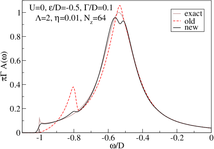
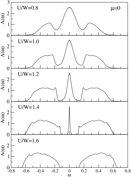
The most severe shortcoming of the NRG (using log-Gaussian broadening with large and traditional discretization schemes) in its role as an impurity solver in DMFT was the reduced energy resolution at finite excitation energies. This not only affects the self-consistent calculation by introducing systematic errors, but sometimes features in spectral functions at high energies (for example kinks in the excitation dispersions) are themselves of interest. We demonstrate the applicability of the new approach on the simplest example of the Hubbard model. The case of hypercubic lattice is considered in Fig. 17 where we plot the local density of states for a range of the repulsion parameter as the metal-insulator transition is approached. Compared to the results computed using the conventional NRG approach, the high-energy features (Hubbard bands) are sharper. Furthermore, the conventional approach underestimates the reduction of the density of states (“pseudo-gap”) between the Hubbard bands and the quasiparticle peak. We also observe that the Hubbard bands have inner structure. We find a notable peak at the inner edges of the Hubbard band; the existence of some spectral features at the band edges had been suggested already in the early iterative perturbation theory, non-crossing approximation, quantum Monte Carlo and NRG DMFT results for the Hubbard model and the existence of a sharp peak was demonstrated in more recent high-resolution dynamic density-matrix renormalization (D-DMRG) calculations Karski et al. (2005, 2008).
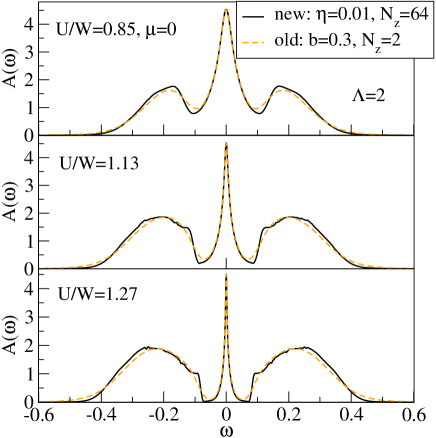
On the Bethe lattice, Fig. 18, the Hubbard bands are sharper due to the finite support of the lattice density of states and the inner Hubbard band edge peaks are sharper. There are furthermore less pronounced spectral features at integer multiples of the energy of the inner Hubbard band edge; they are most visible in the results. We also calculated the local two-particle Green functions at the end of the DMFT cycle to try to obtain some insight whether these additional structures are possibly related to certain two-particle excitations. However, no clear evidence was found for such statement. Thus, at present, we cannot give a satisfactory physical explanation of these additional structures. In any case, they motivate further high-resolution studies of both the single-impurity Anderson model and the Hubbard model in DMFT, concentrating on the regime with vanishing Kondo resonance.
X Conclusion
We presented spectral function calculations which indicate that the numerical renormalization group method allows to compute more accurate results than it is generally believed. We have shown that overbroadening effects can be in large part removed by using a sufficiently narrow Gaussian broadening kernel. Furthermore, we have shown that there is surprisingly little variation as is decreased (disregarding the artefact shifts), thus there is no inherent overbroadening due to the discretization of the conduction band. At best one can say that as is increased, more values need to be used in the interleaved method to obtain smooth spectral functions. It must be emphasized that sweeping over is an embarrassingly parallel problem, i.e. essentially no overhead is associated with splitting the problem into a large number of parallel tasks.
As the continuum limit is approached (), the discretization artefacts in the spectral function calculated using the traditional schemes shift out toward the band-edge, but in the range of that can be used in practical calculations, the artefacts are always present. The use of the logarithmic discretization is commonly justified by the rapid convergence of calculated quantities to the continuum limit; while static properties indeed converge rapidly, this is not the case with dynamic properties. The presence of artefacts therefore has several implications for NRG calculation. First of all, in the traditional approach it cannot be claimed that a calculation is performed for a given density of states , but rather for a band with a density of states given by in the problem with decoupled impurity. The presence of the structure in the spectral function then forcibly leads to what is perceived as “artefacts” in the impurity spectral function . Artefacts have important implications for the application of the NRG in DMFT, since these anomalies lead to features in the impurity spectral function that are difficult to disassociate from real fine structure. A good test to distinguish between artefacts and real spectral features is to perform calculations for several values of , keeping all other parameters constant. Real features will change very little, while artefacts will shift and change form significantly. Depending on the circumstances (structure of the impurity model, model parameters) and the purposes (single-impurity calculation vs. self-consistent dynamical mean-field-theory calculation), the artefacts are either benign or rather detrimental.
The proposed new way of calculating the coefficients leads to a sizable improvement in the convergence to the limit and to a significant reduction of the discretization artefacts. Since the DMFT self-consistency loop couples low-energy and high-energy scales, the reduction of the artefacts at high energies is a significant improvement which increases the reliability of the NRG as an impurity solver.
Acknowledgements.
We thank Janez Bonča for providing the motivation which led to this work and Robert Peters for discussions on the calculation of spectral functions. We acknowledge computer support by the Gesellschaft für wissenschaftliche Datenverarbeitung (GWDG) in Göttingen and support by the German Science Foundation through SFB 602.Appendix A Spectral function broadening
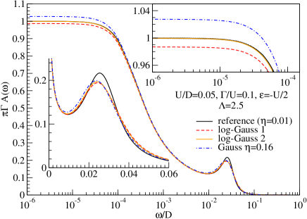
In practical NRG calculations, -averaging is performed over a smaller number of twist parameters, therefore wider broadening functions must be used. It is thus interesting to compare the results for spectral functions obtained using different broadening kernels, Fig. 19. We compare simple Gaussian broadening, conventional log-Gaussian broadening and a modified log-Gaussian kernel proposed in Ref. Weichselbaum and von Delft, 2007:
| (43) |
with . The same , and were use for all three broadening kernels, with .
In the low-energy () range, we find that Gaussian broadening overestimates the spectral density, log-Gaussian broadening underestimates it, while the modified log-Gaussian kernel, Eq. (43), gives a very good approximation to the high-resolution result. All three approaches describe quite well the flanks of the Kondo resonance. Gaussian broadening overestimates the spectral density in the energy range between the Kondo resonance and the Hubbard peak, while the best results are here obtained by the original log-Gaussian broadening. All three broadening approaches shift the maximum of the Hubbard peak to lower energies to roughly comparable degree. Finally, in the high-energy range, log-Gaussian approaches overestimate the spectral density more than the simple Gaussian broadening.
For studying low-energy properties with typical NRG broadening parameters, the modified log-Gaussian kernel, Eq. (43), is the best choice. For high-resolution studies with very small broadening, all three broadening techniques become almost equivalent, but the plain Gaussian kernel has a small advantage by being symmetric; the symmetry leads to smaller deviations of higher-moment spectral sum rules.
Appendix B Modified discretization scheme
We describe the modified discretization scheme which consists of solving the ordinary differential equation for :
| (44) |
As a first step, we introduce continuous indexing as with parameter running from 1 to , so that coefficients and become continuous functions of , i.e. and . We then rewrite Eq. (44) as
| (45) |
with the initial condition . It is helpful to take into account the expected asymptotic behavior of using the following Ansatz:
| (46) |
with . The equation to solve is then
| (47) |
This equation can be solved numerically; for general it is advisable to use arbitrary-precision numerics for this purpose, since the equation is stiff. For DOS which is finite at the Fermi level, we must have . Checking the convergence to this value is a good test of the integration procedure.
References
- Wilson (1975) K. G. Wilson, Rev. Mod. Phys. 47, 773 (1975).
- Krishna-murthy et al. (1980a) H. R. Krishna-murthy, J. W. Wilkins, and K. G. Wilson, Phys. Rev. B 21, 1003 (1980a).
- Bulla et al. (2008) R. Bulla, T. Costi, and T. Pruschke, Rev. Mod. Phys. 80, 395 (2008).
- Hofstetter (2000) W. Hofstetter, Phys. Rev. Lett. 85, 1508 (2000).
- Sakai et al. (1989) O. Sakai, Y. Shimizu, and T. Kasuya, J. Phys. Soc. Japan 58, 3666 (1989).
- Bulla et al. (1998) R. Bulla, A. C. Hewson, and T. Pruschke, J. Phys.: Condens. Matter 10, 8365 (1998).
- Peters et al. (2006) R. Peters, T. Pruschke, and F. B. Anders, Phys. Rev. B 74, 245114 (2006).
- Weichselbaum and von Delft (2007) A. Weichselbaum and J. von Delft, Phys. Rev. Lett. 99, 076402 (2007).
- Sakai and Shimizu (1992) O. Sakai and Y. Shimizu, J. Phys. Soc. Japan 61, 2333 (1992).
- Costi et al. (1994) T. A. Costi, A. C. Hewson, and V. Zlatic, J. Phys.: Condens. Matter 6, 2519 (1994).
- Krishna-murthy et al. (1980b) H. R. Krishna-murthy, J. W. Wilkins, and K. G. Wilson, Phys. Rev. B 21, 1044 (1980b).
- Oliveira and Wilkins (1981) L. N. Oliveira and J. W. Wilkins, Phys. Rev. Lett. 47, 1553 (1981).
- Satori et al. (1992) K. Satori, H. Shiba, O. Sakai, and Y. Shimizu, J. Phys. Soc. Japan 61, 3239 (1992).
- Sakai et al. (1993) O. Sakai, Y. Shimizu, H. Shiba, and K. Satori, J. Phys. Soc. Japan 62, 3181 (1993).
- Costi and Kieffer (1996) T. A. Costi and C. Kieffer, Phys. Rev. Lett. 76, 1683 (1996).
- Izumida et al. (1998) W. Izumida, O. Sakai, and Y. Shimizu, J. Phys. Soc. Japan 67, 2444 (1998).
- Sakai and Kuramoto (1994) O. Sakai and Y. Kuramoto, Solid State Commun. 89, 307 (1994).
- Bulla (1999) R. Bulla, Phys. Rev. Lett. 83, 136 (1999).
- Pruschke et al. (2000) T. Pruschke, R. Bulla, and M. Jarrell, Phys. Rev. B 61, 12799 (2000).
- Georges et al. (1996) A. Georges, G. Kotliar, W. Krauth, and M. J. Rozenberg, Rev. Mod. Phys. 68, 13 (1996).
- Campo and Oliveira (2005) V. L. Campo and L. N. Oliveira, Phys. Rev. B 72, 104432 (2005).
- Bulla et al. (2005) R. Bulla, H.-J. Lee, N.-H. Tong, and M. Vojta, Phys. Rev. B 71, 045122 (2005).
- Bulla et al. (2001) R. Bulla, T. A. Costi, and D. Vollhardt, Phys. Rev. B 64, 045103 (2001).
- Oliveira and Oliveira (1994) W. C. Oliveira and L. N. Oliveira, Phys. Rev. B 49, 11986 (1994).
- Silva et al. (1996) J. B. Silva, W. L. C. Lima, W. C. Oliveira, J. L. N. Mello, L. N. Oliveira, and J. W. Wilkins, Phys. Rev. Lett. 76, 275 (1996).
- Paula et al. (1999) C. A. Paula, M. F. Silva, and L. N. Oliveira, Phys. Rev. B 59, 85 (1999).
- Anderson (1961) P. W. Anderson, Phys. Rev. 124, 41 (1961).
- Žitko and Bonča (2006a) R. Žitko and J. Bonča, Phys. Rev. B 73, 035332 (2006a).
- Tóth et al. (2008) A. I. Tóth, C. P. Moca, O. Legeza, and G. Zaránd, Density matrix numerical renormalization group for non-abelian symmetries, arXiv:0802.4332 (2008).
- Costi and Hewson (1992) T. A. Costi and A. C. Hewson, Phil. Mag. B 65, 1165 (1992).
- White (1991) S. White, Phys. Rev. B 44, 4670 (1991).
- Yoshida et al. (1990) M. Yoshida, M. A. Whitaker, and L. N. Oliveira, Phys. Rev. B 41, 9403 (1990).
- Raas and Uhrig (2005) C. Raas and G. S. Uhrig, Eur. Phys. J. B 45, 293 (2005).
- Bulla et al. (2000) R. Bulla, M. T. Glossop, D. E. Logan, and T. Pruschke, J. Phys.: Condens. Matter 12, 4899 (2000).
- Dickens and Logan (2001) N. L. Dickens and D. E. Logan, J. Phys.: Condens. Matter 13, 4505 (2001).
- Glossop and Logan (2002) M. T. Glossop and D. E. Logan, J. Phys.: Condens. Matter 14, 6737 (2002).
- Rosch et al. (2003) A. Rosch, T. A. Costi, J. Paaske, and P. Wölfle, Phys. Rev. B 68, 014430 (2003).
- Micklitz et al. (2006) T. Micklitz, A. Altland, T. A. Costi, and A. Rosch, Phys. Rev. Lett. 96, 226601 (2006).
- Hewson and Meyer (2002) A. C. Hewson and D. Meyer, J. Phys. - Condens. Mat. 14, 427 (2002).
- Jeon et al. (2003) G. S. Jeon, T.-H. Park, and H.-Y. Choi, Phys. Rev. B 68, 045106 (2003).
- Cornaglia et al. (2004) P. S. Cornaglia, H. Ness, and D. R. Grempel, Phys. Rev. Lett. 93, 147201 (2004).
- Cornaglia et al. (2005) P. S. Cornaglia, D. R. Grempel, and H. Ness, Phys. Rev. B 71, 075320 (2005).
- Žitko and Bonča (2006b) R. Žitko and J. Bonča, Phys. Rev. B 74, 224411 (2006b).
- Mahan (2000) G. D. Mahan, Many-particle physics (Kluwer Academic, New York, 2000).
- Karski et al. (2005) M. Karski, C. Raas, and G. S. Uhrig, Phys. Rev. B 72, 113110 (2005).
- Karski et al. (2008) M. Karski, C. Raas, and G. S. Uhrig, Phys. Rev. B 77, 075116 (2008).