Robust Estimation of Mean Values

Abstract

In this paper, we develop a computational approach for estimating the mean value of a quantity in the presence of uncertainty. We demonstrate that, under some mild assumptions, the upper and lower bounds of the mean value are efficiently computable via a sample reuse technique, of which the computational complexity is shown to posses a Poisson distribution.

1 Introduction

In many situations, it is desirable to estimate the mean value of a scalar quantity $\boldsymbol{Q}$ which is a function of independent random vectors $\boldsymbol{V}$ and $\boldsymbol{\varDelta}$ such that the distribution of $\boldsymbol{V}$ is known and that the distribution of $\boldsymbol{\varDelta}$ is unknown [4]. Namely, it is interested to estimate the expectation of $\boldsymbol{Q}=q(\boldsymbol{V},\boldsymbol{\varDelta})$, where $q(.,.)$ is a multivariate function. From modeling considerations, it is reasonable to assume that $\boldsymbol{\varDelta}$ is bounded in norm $||.||$, and radially symmetrical and nondecreasing in its probability density function, $f_{\boldsymbol{\varDelta}}(.)$ with the following notions:

(i) The norm, $||\boldsymbol{\varDelta}||$, of $\boldsymbol{\varDelta}$ is no greater than a certain value $r$, i.e., $||\boldsymbol{\varDelta}||\leq r$;

(ii) For any realization $\varDelta$ of $\boldsymbol{\varDelta}$, $f_{\boldsymbol{\varDelta}}(\varDelta)$ depends only on, $||\varDelta||$, the norm of $\varDelta$;

(iii) For any $\varDelta_{1}$ and $\varDelta_{2}$ such that $||\varDelta_{1}||<||\varDelta_{2}||$, $f_{\boldsymbol{\varDelta}}(\varDelta_{1})\geq f_{\boldsymbol{\varDelta}}(\varDelta_{2})$.

Such assumptions have been proposed by Barmish and Lagoa [1] in the context of robustness analysis of control systems, where $\boldsymbol{\varDelta}$ is referred to as “uncertainty” because of the lack of knowledge of its distribution.

In this paper, we shall focus on the estimation of the expectation $\mathbb{E}[\boldsymbol{Q}]=\mathbb{E}[q(\boldsymbol{V},\boldsymbol{\varDelta})]$ based on assumptions (i), (ii) and (iii). Such a problem is referred to as robust estimation due to the fact that the exact distribution of $\boldsymbol{\varDelta}$ is not available. In the special case that the maximum norm $r$ of $\boldsymbol{\varDelta}$ equals $0$, the robust estimation problem reduces to a conventional estimation problem. Instead of seeking the exact value of $\mathbb{E}[\boldsymbol{Q}]$ which is obviously impossible, we aim at obtaining upper and lower bounds for $\mathbb{E}[\boldsymbol{Q}]$. It is intuitive that the gap between the upper and lower bounds should be increasing with respect to $r$. Since the relation between $Q$ and $\boldsymbol{V},\;\boldsymbol{\varDelta}$ can be fairly complicated, the Monte Carlo estimation method is the unique and powerful approach.

The remainder of the paper is organized as follows. In Section 2, we derive upper and lower bounds for $\mathbb{E}[\boldsymbol{Q}]$ based on assumptions (i), (ii) and (iii). In Section 3, we propose a Monte Carlo method for the evaluation of the bounds of $\mathbb{E}[\boldsymbol{Q}]$. In particular, we introduce a sample reuse method to substantially reduce the computational complexity. In Section 4, we investigate the computational complexity of the Monte Carlo method implemented with the principle of sample reuse. Section 5 is the conclusion.

2 Bounds of Expectation

In this section, we shall derive upper and lower bounds of $\mathbb{E}[\boldsymbol{Q}]=\mathbb{E}[q(\boldsymbol{V},\boldsymbol{\varDelta})]$ based on the assumptions described in Section 1. For this purpose, we have the following fundamental result, which is a slight generalization of the uniform principle proposed by Barmish and Lagoa [1].

Theorem 1

Let $\boldsymbol{\varDelta}_{\rho}^{\mathrm{u}}$ be a random vector with a uniform distribution over $\{\varDelta:||\varDelta||\leq\rho\}$. Define

$$\mathbb{M}(\rho)=\mathbb{E}\left[q(\boldsymbol{V},\boldsymbol{\varDelta}_{\rho}^{\mathrm{u}})\right],\quad\underline{\mathbb{M}}(r)=\inf_{0<\rho<r}\mathbb{M}(\rho),\quad\overline{\mathbb{M}}(r)=\sup_{0<\rho<r}\mathbb{M}(\rho).$$

Then, $\underline{\mathbb{M}}(r)<\mathbb{E}[\boldsymbol{Q}]<\overline{\mathbb{M}}(r)$.

See Appendix A for a proof. Theorem 1 reveals that the computation of the bounds of $\mathbb{E}[\boldsymbol{Q}]$ can be reduced to the evaluation of function $\mathbb{M}(\rho)$, which can be accomplished via Monte Carlo simulation. A conventional method is as follows:

Partition interval $(0,r]$ by grid points $r=\rho_{1}>\rho_{2}>\cdots>\rho_{m}>0$. Let $\mathscr{B}_{\ell}=\{\varDelta:||\varDelta||\leq\rho_{\ell}\}$. For $\ell=1,\cdots,m$, estimate $\mathbb{M}(\rho_{\ell})$ as the empirical mean

$$\frac{\sum_{i=1}^{N}q(\boldsymbol{V}_{i},X_{\ell,i})}{N}$$

where $\boldsymbol{V}_{i},\;X_{\ell,i},\;i=1,\cdots,N$ are mutually independent random variables such that $\boldsymbol{V}_{1},\cdots,\boldsymbol{V}_{N}$ are i.i.d. random samples of $\boldsymbol{V}$ and $X_{\ell,1},\cdots,X_{\ell,N}$ are i.i.d. random samples uniformly distributed over $\mathscr{B}_{\ell}$. Clearly, the total number of simulations is $Nm$ for estimating $\mathbb{M}(\rho_{\ell}),\;\ell=1,\cdots,m$. A major problem with this approach is that the computational complexity can be extremely high, since the number of grid points $m$ is typically a very large number. To overcome such a problem, we shall develop a sample reuse technique in the next section.

3 Sample Reuse

In this section, we shall explore the idea of sample reuse to reduce the computational complexity. The sample reuse method has been proposed by Chen et al. [2, 3] for the robustness analysis of control systems. The idea of sample reuse is to start simulation from the largest set $\mathscr{B}_{1}$ and if it also belongs to smaller subsets the experimental result is saved for later use in the smaller sets. As can be seen from last section, a conventional approach would require a total of $Nm$ simulations. However, due to sample reuse, the actual number of experiments for set $\mathscr{B}_{\ell}$ is a random number $\mathbf{n}_{\ell}$, which is usually much less than $N$. Hence, this strategy saves a significant amount of computational effort.

In order to provide a precise description of the principle of sample reuse, we assume that all random variables are defined in the same probability space $(\Omega,\mathscr{F},\Pr)$. We shall introduce a function $\mathscr{G}$, referred to as sample reuse function, as follows.

Let $X_{1},\cdots,X_{m}$ be i.i.d. samples uniformly distributed over $\mathscr{A}$. Let $Y_{1},\cdots,Y_{n}$ be i.i.d. samples uniformly distributed over $\mathscr{B}$. Let $m\leq n$ and $\mathscr{A}\supset\mathscr{B}$. Define reusable sample size $\mathbf{k}$ such that $\mathbf{k}(\omega)$ is the number of elements of $\{X_{i}(\omega)\in\mathscr{B}:i=1,\cdots,m\}$ for any $\omega\in\Omega$. Define random variables $Z_{1},\cdots,Z_{n}$ such that, for any $\omega\in\Omega$,

$$Z_{\ell}(\omega)=\begin{cases}X_{i_{\ell}}(\omega)&\text{for}\;1\leq\ell\leq\mathbf{k}(\omega),\\ Y_{\ell}(\omega)&\text{for}\;\mathbf{k}(\omega)<\ell\leq n\end{cases}$$

where $i_{\ell},\;1\leq\ell\leq\mathbf{k}(\omega)$ are the indexes of the elements of $\{X_{i}(\omega)\in\mathscr{B}:i=1,\cdots,n\}$ such that $i_{\ell}$ is increasing with respect to $\ell$. This process of generating $Z_{1},\cdots,Z_{n}$ from $X_{1},\cdots,X_{m}$ and $Y_{1},\cdots,Y_{n}$ is denoted by

$$(Z_{1},\cdots,Z_{n};\mathbf{k})=\mathscr{G}(X_{1},\cdots,X_{m};Y_{1},\cdots,Y_{n}).$$

With regard to the distribution of $Z_{1},\cdots,Z_{n}$, we have

Theorem 2

Suppose $X_{1},\cdots,X_{m}$ are independent with $Y_{1},\cdots,Y_{n}$. Then, $Z_{1},\cdots,Z_{n}$ are i.i.d. samples uniformly distributed over $\mathscr{B}$.

See Appendix B for a proof. Now we can use $\mathscr{G}$ to precisely describe the sample reuse algorithm for estimating $\mathbb{M}(\rho_{\ell}),\;\ell=1,\cdots,m$. Let $X_{\ell,i},\;i=1,\cdots,N$ be the random samples uniformly distributed over $\mathscr{B}_{\ell}$ for $\ell=1,\cdots,m$. Let $Y_{1,i}=X_{1,i}$ for $i=1,\cdots,N$ and $(Y_{\ell,1},\cdots,Y_{\ell,N};\mathbf{k}_{\ell})=\mathscr{G}(Y_{\ell-1,1},\cdots,Y_{\ell-1,N};X_{\ell,1},\cdots,X_{\ell,N})$ for $\ell=2,\cdots,m$. As a result of Theorem 1, we have that, for any $\ell\in\{1,\cdots,m\}$, random variables $Y_{\ell,i},\;i=1,\cdots,N$ have the same associated cumulative distribution with that of random variables $X_{\ell,i},\;i=1,\cdots,N$. This implies that $\frac{1}{N}\sum_{i=1}^{N}q(\boldsymbol{V}_{i},Y_{\ell,i})$ has the same distribution as that of $\frac{1}{N}\sum_{i=1}^{N}q(\boldsymbol{V}_{i},X_{\ell,i})$ for $\ell=1,\cdots,m$. Therefore, we can use $\frac{1}{N}\sum_{i=1}^{N}q(\boldsymbol{V}_{i},Y_{\ell,i})$ as an estimator of $\mathbb{M}(\rho_{\ell})$ for $\ell=1,\cdots,m$. By virtue of such sample reuse method, the total number of simulations is reduced from $Nm$ to $N+\sum_{\ell=2}^{m}\mathbf{n}_{\ell}$, where $\mathbf{n}_{\ell}=N-\mathbf{k}_{\ell}$ for $\ell=2,\cdots,m$. As will be demonstrated in the next section, this can be a huge reduction of complexity for a large $m$.

4 Poisson Complexity

Since the total number of simulations for using the sample reuse method to estimate $\mathbb{M}(\rho_{\ell}),\;\ell=1,\cdots,m$ is $N+\sum_{\ell=2}^{m}\mathbf{n}_{\ell}$, it is important to investigate the distribution of $\sum_{\ell=2}^{m}\mathbf{n}_{\ell}$. In this regard, we have the following general result.

Theorem 3

For arbitrary sequence of nested sets $\mathscr{B}_{1}\supset\mathscr{B}_{2}\supset\cdots\supset\mathscr{B}_{m}$ with $\mathrm{vol}(\mathscr{B}_{1})=V_{\mathrm{max}}$ and $\mathrm{vol}(\mathscr{B}_{m})=V_{\mathrm{min}}$, the cumulative distribution function of $\sum_{\ell=2}^{m}\mathbf{n}_{\ell}$ is bounded from below by the cumulative distribution function of a Poisson random variable $\boldsymbol{P}$ with mean $\lambda=N\ln\left(\frac{V_{\mathrm{max}}}{V_{\mathrm{min}}}\right)$. That is, $\Pr\left\{\sum_{\ell=2}^{m}\mathbf{n}_{\ell}=0\right\}=\Pr\{\boldsymbol{P}=0\}$ and $\Pr\left\{\sum_{\ell=2}^{m}\mathbf{n}_{\ell}\leq k\right\}>\Pr\{\boldsymbol{P}\leq k\}$ for any positive integer $k$. Moreover, as the maximum difference of volumes of all consecutive sets tends to be zero, $\sum_{\ell=2}^{m}\mathbf{n}_{\ell}$ converges to $\boldsymbol{P}$ in distribution.

See Appendix C for a proof. It should be noted that the volume of a set $\mathscr{B}$, denoted by $\mathrm{vol}(\mathscr{B})$, is referred to the Lebesgue measure of $\mathscr{B}$ in this paper.

As an immediate consequence of Theorem 3, we have

$$\Pr\left\{\sum_{\ell=2}^{m}\mathbf{n}_{\ell}>0\right\}=\Pr\{\boldsymbol{P}>0\},\qquad\Pr\left\{\sum_{\ell=2}^{m}\mathbf{n}_{\ell}>k\right\}<\Pr\{\boldsymbol{P}>k\},\quad k=1,2,\cdots$$

which implies that

$$\mathbb{E}\left[\sum_{\ell=2}^{m}\mathbf{n}_{\ell}\right]=\sum_{k=0}^{\infty}\Pr\left\{\sum_{\ell=2}^{m}\mathbf{n}_{\ell}>k\right\}<\sum_{k=0}^{\infty}\Pr\{\boldsymbol{P}>k\}=\lambda=N\ln\left(\frac{V_{\mathrm{max}}}{V_{\mathrm{min}}}\right).$$

By virtue of Theorem 3, we can derive some simple bounds for the distribution of $\sum_{\ell=2}^{m}\mathbf{n}_{\ell}$ as follows.

Theorem 4

$\Pr\{\sum_{\ell=2}^{m}\mathbf{n}_{\ell}\geq k\}\leq e^{-\lambda}\left(\frac{\lambda e}{k}\right)^{k}$ for any number $k>\lambda=N\ln\left(\frac{V_{\mathrm{max}}}{V_{\mathrm{min}}}\right)$. In particular, $\Pr\{\sum_{\ell=2}^{m}\mathbf{n}_{\ell}\geq e\lambda\}\leq e^{-\lambda}$ and $\Pr\{X\geq(1+\epsilon)\lambda\}<\exp\left(-\frac{\epsilon^{2}\lambda}{4}\right)$ for $0<\epsilon<1$.

See Appendix D for a proof.

Now we apply Theorem 3 to investigate the density of original samples of $\boldsymbol{\varDelta}$. Suppose that the volume of $\{\varDelta:||\varDelta||\leq\rho\}$ is proportional to $\rho^{d}$ where $d$ is the dimension of the set. Let $\boldsymbol{N}_{\rho}$ denote the number of original samples included in $\{\varDelta:||\varDelta||\leq\rho\}$ when applying the sample reuse method to interval $[\frac{\rho}{\kappa},\rho]$. Define the density of samples at radius $\rho$ as $\mathcal{D}(\rho)=\lim_{\delta\to 0}\frac{\mathbb{E}[\boldsymbol{N}_{\rho+\delta}-\boldsymbol{N}_{\rho}]}{\delta}$. Then, we have the following result.

Theorem 5

$\mathcal{D}(\rho)$ is equal to $\frac{Nd}{\rho}\left(\frac{\kappa\rho}{a}\right)^{d}$ for $\rho\in(0,\frac{a}{\kappa}]$ and is less than $\frac{Nd}{\rho}$ for $\rho\in(\frac{a}{\kappa},a]$.

See Appendix E for a proof. From this theorem, we can obtain an upper bound for the expected number of original samples with norm bounded in $[0,a]$. As can be seen from Theorem 5, the density function is unimodal and achieves the largest value at $\rho=\frac{a}{\kappa}$. The density function is displayed by Figure 1.

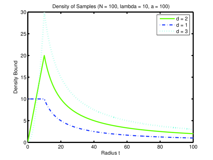
Figure 1: Illustrative Example ($N=100,\;a=100,\;\lambda=10$)

5 Conclusion

We have proposed an efficient computational approach for estimating the mean value of a random function, for which the distribution of relevant random variables are not completely available. A Monte Carlo method with sample reuse as a key mechanism is established. The associated computational complexity is demonstrated to follow a Poisson distribution.

Appendix A Proof of Theorem 1

We follow the similar method of Barmish and Lagoa [1]. Let $\mathcal{V}$ denote the volume of $\mathcal{B}=\{\varDelta:||\varDelta||\leq r\}$. We partition the set $\mathcal{B}$ as $K$ layers of equal volume $\frac{\mathcal{V}}{K}$ such that the $k$-th layer is $\mathcal{L}_{k}=\{\varDelta:r_{k-1}<||\varDelta||\leq r_{k}\}$ with $0=r_{0}<r_{1}<r_{2}<\cdots<r_{K}=r$. Then, the density function can be expressed as

$$f_{\boldsymbol{\varDelta}}(\Delta)\approx\sum_{k=1}^{K}\mathbb{I}_{k}(\Delta)\lambda_{k}$$

where $\lambda_{k},\;k=1,\cdots,K$ satisfying

$$\frac{\mathcal{V}}{K}\sum_{k=1}^{K}\lambda_{k}=1,\qquad\lambda_{1}\geq\lambda_{2}\geq\cdots\geq\lambda_{K}\geq 0$$ (1)

and $\mathbb{I}_{k}(.)$ is the indicator function such that $\mathbb{I}_{k}(\Delta)=1$ if $\Delta$ falls into the $k$-th layer $\mathcal{L}_{k}$ and $\mathbb{I}_{k}(\Delta)=0$ otherwise. Let $f_{\boldsymbol{V}}(.)$ denote the density function of $\boldsymbol{V}$. Since $\boldsymbol{V}$ and $\boldsymbol{\varDelta}$ are independent, we have

$$\mathbb{E}[q(\boldsymbol{V},\boldsymbol{\varDelta})] \approx \int_{\{(v,\Delta):||\Delta||\leq r\}}q(v,\Delta)\;f_{\boldsymbol{V}}(v)dv\;f_{\boldsymbol{\varDelta}}(\Delta)d\Delta$$

$$= \int_{\{(v,\Delta):||\Delta||\leq r\}}q(v,\Delta)\;f_{\boldsymbol{V}}(v)dv\;\left[\sum_{k=1}^{K}\mathbb{I}_{k}(\Delta)\lambda_{k}\right]d\Delta=\sum_{k=1}^{K}\alpha_{k}\lambda_{k},$$

where $\alpha_{k}=\int_{\{(v,\Delta):||\Delta||\leq r\}}q(v,\Delta)\;\mathbb{I}_{k}(\Delta)f_{\boldsymbol{V}}(v)dv\;d\Delta$. Therefore, the upper and lower bounds of $\mathbb{E}[q(\boldsymbol{V},\boldsymbol{\varDelta})]$ correspond to the maximum and minimum of the linear program: $\sum_{k=1}^{K}\alpha_{k}\lambda_{k}$ subject to constraint (1). From convex analysis, the maximum and minimum of this linear program are achieving at extreme points of the form:

$$\lambda_{k}=\begin{cases}\frac{K}{j\mathcal{V}}&\text{for}\;1\leq k\leq j,\\ 0&\text{for}\;j<k\leq K.\end{cases}$$

As the number of layers $K$ tends to infinity, the summation $\sum_{k=1}^{K}\mathbb{I}_{k}(\Delta)\lambda_{k}$, which is associated with extreme point $(\lambda_{1},\cdots,\lambda_{K})$, tends to a uniform distribution. This justifies the theorem.

Appendix B Proof of Theorem 2

Let $S_{\ell}\subseteq{\mathscr{B}}$ for $\ell=1,\cdots,n$. Define $\mathbb{D}=\{1,\cdots,n\}$ and $\mathcal{I}_{s}=\{(i_{1},\cdots,i_{s}):i_{1}<\cdots<i_{s};\;i_{\ell}\in\mathbb{D},\;\ell=1,\cdots,s\}$. Then,

$$\Pr\{Z_{\ell}\in S_{\ell},\;\ell=1,\cdots,n\} = \sum_{s=0}^{n}\sum_{(i_{1},\cdots,i_{s})\in\mathcal{I}_{s}}\Pr\{X_{i_{\ell}}\in S_{\ell},\;\ell=1,\cdots,s;\;X_{j}\notin{\mathscr{B}},\;j\in\mathbb{D}\setminus\{i_{1},\cdots,i_{s}\}\}$$

$$\times\Pr\{Y_{\ell}\in S_{\ell},\;\ell=s+1,\cdots,n\}.$$

For simplicity of notations, we let $V_{S_{\ell}}=\mathrm{vol}(S_{\ell}),\;V_{\mathscr{A}}=\mathrm{vol}(\mathscr{A})$ and $V_{\mathscr{B}}=\mathrm{vol}(\mathscr{B})$. Note that $\Pr\{Y_{\ell}\in S_{\ell},\;\ell=s+1,\cdots,n\}=\prod_{\ell=s+1}^{n}\left(\frac{V_{S_{\ell}}}{V_{\mathscr{B}}}\right)$ and

$$\Pr\{X_{i_{\ell}}\in S_{\ell},\;\ell=1,\cdots,s;\;X_{j}\notin{\mathscr{B}},\;j\in\mathbb{D}\setminus\{i_{1},\cdots,i_{s}\}\} = \left(\frac{V_{\mathscr{A}}-V_{\mathscr{B}}}{V_{\mathscr{A}}}\right)^{m-s}\prod_{\ell=1}^{s}\left(\frac{V_{S_{\ell}}}{V_{\mathscr{A}}}\right)$$

$$= \left(\frac{V_{\mathscr{B}}}{V_{\mathscr{A}}}\right)^{s}\left(1-\frac{V_{\mathscr{B}}}{V_{\mathscr{A}}}\right)^{m-s}\prod_{\ell=1}^{s}\left(\frac{V_{S_{\ell}}}{V_{\mathscr{B}}}\right).$$

Since there are $\binom{n}{s}$ elements in $\mathcal{I}_{s}$, we have

$$\Pr\{Z_{\ell}\in S_{\ell},\;\ell=1,\cdots,n\} = \sum_{s=0}^{n}\binom{n}{s}\left(\frac{V_{\mathscr{B}}}{V_{\mathscr{A}}}\right)^{s}\left(1-\frac{V_{\mathscr{B}}}{V_{\mathscr{A}}}\right)^{m-s}\prod_{\ell=1}^{s}\left(\frac{V_{S_{\ell}}}{V_{\mathscr{B}}}\right)\prod_{\ell=s+1}^{n}\left(\frac{V_{S_{\ell}}}{V_{\mathscr{B}}}\right)$$

$$= \prod_{\ell=1}^{n}\left(\frac{V_{S_{\ell}}}{V_{\mathscr{B}}}\right)\sum_{s=0}^{n}\binom{n}{s}\left(\frac{V_{\mathscr{B}}}{V_{\mathscr{A}}}\right)^{s}\left(1-\frac{V_{\mathscr{B}}}{V_{\mathscr{A}}}\right)^{m-s}$$

$$= \prod_{\ell=1}^{n}\left(\frac{V_{S_{\ell}}}{V_{\mathscr{B}}}\right).$$

This concludes the proof of the theorem.

Appendix C Proof of Theorem 3

We need some preliminary results.

Lemma 1

Let $N_{1}\leq N_{2}\leq\cdots\leq N_{m}$. For $\ell=1,\cdots,m$, let $v_{\ell}=\mathrm{vol}(\mathscr{B}_{\ell})$ and $X_{\ell,i},\;i=1,\cdots,N_{\ell}$ be i.i.d. random samples uniformly distributed over $\mathscr{B}_{\ell}$. Let $Y_{1,i}=X_{1,i}$ for $i=1,\cdots,N_{1}$ and $(Y_{\ell,1},\cdots,Y_{\ell,N_{\ell}};\mathbf{k}_{\ell})=\mathscr{G}(Y_{\ell-1,1},\cdots,Y_{\ell-1,N_{\ell-1}};X_{\ell,1},\cdots,X_{\ell,N_{\ell}})$ for $\ell=2,\cdots,m$. Define $\mathbf{n}_{\ell}=N_{\ell}-\mathbf{k}_{\ell}$ for $\ell=2,\cdots,m$. Then, $\Pr\{\mathbf{n}_{\ell}=n_{\ell},\;\ell=2,\cdots,m\}=\prod_{\ell=2}^{m}B\left(N_{\ell}-n_{\ell},N_{\ell-1},\frac{v_{\ell}}{v_{\ell-1}}\right)$ for $N_{\ell}-N_{\ell-1}\leq n_{\ell}\leq N_{\ell}$ and $2\leq\ell\leq m$, where $B(k,n,p)=\binom{n}{k}p^{k}(1-p)^{n-k}$.

Proof.

We use induction method. First, it is easy to show that the lemma is true for $m=2$. Next, we assume that the lemma is true for $m-1$ and show that the lemma is also true for $m$. Let $\Pr\{(k_{1},\cdots,k_{m}),\;(N_{1},\cdots,N_{m}),\;(v_{1},\cdots,v_{m})\}$ denote the probability that, among the $N_{1}$ samples generated from the biggest set $\mathscr{B}_{1}$, there are $k_{\ell}$ samples falling into $\mathscr{B}_{\ell}$ for $\ell=1,2,\cdots,m$. Let $\mathbf{P}^{m}\left\{(n_{2},\cdots,n_{m}),\;(N_{1},\cdots,N_{m}),\;(v_{1},\cdots,v_{m})\right\}$ denote the probability of event $\{\mathbf{n}_{\ell}=n_{\ell},\;\ell=2,\cdots,m\}$ associated with the application of the sample reuse method to sets $\mathscr{B}_{\ell},\;\ell=1,\cdots,m$ with required sample sizes $N_{1}\leq N_{2}\leq\cdots\leq N_{m}$. Let $\mathbf{P}^{m-1}\{(n_{3},\cdots,n_{m}),\;(N_{2}-k_{2},\cdots,N_{m}-k_{m}),\;(v_{2},\cdots,v_{m})\}$ denote the probability of event $\{\mathbf{n}_{\ell}=n_{\ell},\;\ell=3,\cdots,m\}$ associated with the application of the sample reuse method to sets $\mathscr{B}_{\ell},\;\ell=2,\cdots,m$ with required sample sizes $N_{2}-k_{2}\leq\cdots\leq N_{m}-k_{m}$. Note that

$$\mathbf{P}^{m}\left\{(n_{2},\cdots,n_{m}),\;(N_{1},\cdots,N_{m}),\;(v_{1},\cdots,v_{m})\right\}$$

$$= \sum_{k_{2}\geq k_{3}\geq\cdots\geq k_{m}\geq 0}\Pr\{(k_{1},\cdots,k_{m}),\;(N_{1},\cdots,N_{m}),\;(v_{1},\cdots,v_{m})\}$$

$$\times\;\mathbf{P}^{m-1}\left\{(n_{3},\cdots,n_{m}),\;\left(N_{2}-k_{2},\;N_{3}-k_{3},\;\cdots,\;N_{m}-k_{m}\right),\;(v_{2},\cdots,v_{m})\right\}$$

where $n_{2}+k_{2}=N_{2}$ and $k_{1}=N_{1}$. By the mechanism of sample reuse,

$$\Pr\{(k_{1},\cdots,k_{m}),\;(N_{1},\cdots,N_{m}),\;(v_{1},\cdots,v_{m})\}\\ =\left[\prod_{\ell=2}^{m}\binom{k_{\ell-1}}{k_{\ell}}\left(\frac{v_{\ell-1}-v_{\ell}}{v_{1}}\right)^{k_{\ell-1}-k_{\ell}}\right]\left(\frac{v_{m}}{v_{1}}\right)^{k_{m}}.$$

Since $N_{\ell}$ and $-k_{\ell}$ are non-decreasing with respect to $\ell$, we have that $N_{\ell}-k_{\ell}$ is non-decreasing with respect to $\ell$. Hence, by the assumption of induction,

$$\mathbf{P}^{m-1}\left\{(n_{3},\cdots,n_{m}),\;\left(N_{2}-k_{2},\;N_{3}-k_{3},\;\cdots,\;N_{m}-k_{m}\right),\;(v_{2},\cdots,v_{m})\right\}$$

$$= \prod_{\ell=3}^{m}B\left(N_{\ell}-n_{\ell}-k_{\ell},N_{\ell-1}-k_{\ell-1},\frac{v_{\ell}}{v_{\ell-1}}\right)$$

$$= \prod_{\ell=3}^{m}\binom{N_{\ell-1}-k_{\ell-1}}{N_{\ell}-n_{\ell}-k_{\ell}}\left(\frac{v_{\ell}}{v_{\ell-1}}\right)^{N_{\ell}-n_{\ell}-k_{\ell}}\left(1-\frac{v_{\ell}}{v_{\ell-1}}\right)^{N_{\ell-1}-N_{\ell}+n_{\ell}-k_{\ell-1}+k_{\ell}}$$

and consequently,

$$\mathbf{P}^{m}\left\{(n_{2},\cdots,n_{m}),\;(N_{1},\cdots,N_{m}),\;(v_{1},\cdots,v_{m})\right\}$$

$$= \sum_{k_{2}\geq k_{3}\geq\cdots\geq k_{m}\geq 0}\left[\prod_{\ell=2}^{m}\binom{k_{\ell-1}}{k_{\ell}}\left(\frac{v_{\ell-1}-v_{\ell}}{v_{1}}\right)^{k_{\ell-1}-k_{\ell}}\right]\left(\frac{v_{m}}{v_{1}}\right)^{k_{m}}$$

$$\times\prod_{\ell=3}^{m}\binom{N_{\ell-1}-k_{\ell-1}}{N_{\ell}-n_{\ell}-k_{\ell}}\left(\frac{v_{\ell}}{v_{\ell-1}}\right)^{N_{\ell}-n_{\ell}-k_{\ell}}\left(1-\frac{v_{\ell}}{v_{\ell-1}}\right)^{N_{\ell-1}-N_{\ell}+n_{\ell}-k_{\ell-1}+k_{\ell}}$$

$$= \sum_{k_{2}\geq k_{3}\geq\cdots\geq k_{m}\geq 0}\left[\prod_{\ell=2}^{m}\binom{k_{\ell-1}}{k_{\ell}}\binom{N_{\ell-1}-k_{\ell-1}}{N_{\ell}-n_{\ell}-k_{\ell}}\right]$$

$$\times\left(\frac{v_{m}}{v_{1}}\right)^{k_{m}}\prod_{\ell=2}^{m}\left(\frac{v_{\ell-1}-v_{\ell}}{v_{1}}\right)^{k_{\ell-1}-k_{\ell}}\times\prod_{\ell=3}^{m}\left(\frac{v_{\ell}}{v_{\ell-1}}\right)^{N_{\ell}-n_{\ell}-k_{\ell}}\left(1-\frac{v_{\ell}}{v_{\ell-1}}\right)^{N_{\ell-1}-N_{\ell}+n_{\ell}-k_{\ell-1}+k_{\ell}}.$$

Making use of the relationships $k_{1}=N_{1}$ and $k_{2}=N_{2}-n_{2}$, we have

$$\left(\frac{v_{m}}{v_{1}}\right)^{k_{m}}\prod_{\ell=2}^{m}\left(\frac{v_{\ell-1}-v_{\ell}}{v_{1}}\right)^{k_{\ell-1}-k_{\ell}}\times\prod_{\ell=3}^{m}\left(\frac{v_{\ell}}{v_{\ell-1}}\right)^{-k_{\ell}}\left(1-\frac{v_{\ell}}{v_{\ell-1}}\right)^{-k_{\ell-1}+k_{\ell}}$$

$$= \left(v_{1}-v_{2}\right)^{k_{1}-k_{2}}\left(\frac{v_{2}^{k_{2}}}{v_{1}^{N_{1}}}\right)=\left(\frac{v_{2}}{v_{1}}\right)^{N_{2}-n_{2}}\left(1-\frac{v_{2}}{v_{1}}\right)^{N_{1}-N_{2}+n_{2}}$$

and thus

$$\left(\frac{v_{m}}{v_{1}}\right)^{k_{m}}\prod_{\ell=2}^{m}\left(\frac{v_{\ell-1}-v_{\ell}}{v_{1}}\right)^{k_{\ell-1}-k_{\ell}}\times\prod_{\ell=3}^{m}\left(\frac{v_{\ell}}{v_{\ell-1}}\right)^{N_{\ell}-n_{\ell}-k_{\ell}}\left(1-\frac{v_{\ell}}{v_{\ell-1}}\right)^{N_{\ell-1}-N_{\ell}+n_{\ell}-k_{\ell-1}+k_{\ell}}$$

$$= \left(\frac{v_{m}}{v_{1}}\right)^{k_{m}}\prod_{\ell=2}^{m}\left(\frac{v_{\ell-1}-v_{\ell}}{v_{1}}\right)^{k_{\ell-1}-k_{\ell}}\times\prod_{\ell=3}^{m}\left(\frac{v_{\ell}}{v_{\ell-1}}\right)^{-k_{\ell}}\left(1-\frac{v_{\ell}}{v_{\ell-1}}\right)^{-k_{\ell-1}+k_{\ell}}$$

$$\times\prod_{\ell=3}^{m}\left(\frac{v_{\ell}}{v_{\ell-1}}\right)^{N_{\ell}-n_{\ell}}\left(1-\frac{v_{\ell}}{v_{\ell-1}}\right)^{N_{\ell-1}-N_{\ell}+n_{\ell}}$$

$$= \prod_{\ell=2}^{m}\left(\frac{v_{\ell}}{v_{\ell-1}}\right)^{N_{\ell}-n_{\ell}}\left(1-\frac{v_{\ell}}{v_{\ell-1}}\right)^{N_{\ell-1}-N_{\ell}+n_{\ell}}.$$

On the other hand, if the lemma really holds, we have

$$\mathbf{P}^{m}\left\{(n_{2},\cdots,n_{m}),\;(N_{1},\cdots,N_{m}),\;(v_{1},\cdots,v_{m})\right\}$$

$$= \prod_{\ell=2}^{m}B\left(N_{\ell}-n_{\ell},N_{\ell-1},\frac{v_{\ell}}{v_{\ell-1}}\right)=\left[\prod_{\ell=2}^{m}\binom{N_{\ell-1}}{N_{\ell}-n_{\ell}}\right]\left[\prod_{\ell=2}^{m}\left(\frac{v_{\ell}}{v_{\ell-1}}\right)^{N_{\ell}-n_{\ell}}\left(1-\frac{v_{\ell}}{v_{\ell-1}}\right)^{N_{\ell-1}-N_{\ell}+n_{\ell}}\right].$$

Therefore, to show the lemma, it remains to show

$$\sum_{k_{2}\geq k_{3}\geq\cdots\geq k_{m}\geq 0}\left[\prod_{\ell=2}^{m}\binom{k_{\ell-1}}{k_{\ell}}\binom{N_{\ell-1}-k_{\ell-1}}{N_{\ell}-n_{\ell}-k_{\ell}}\right]=\prod_{\ell=2}^{m}\binom{N_{\ell-1}}{N_{\ell}-n_{\ell}}.$$

Using the relationships $k_{1}=N_{1}$ and $k_{2}=N_{2}-n_{2}$, this identity can be reduced to the following identity

$$\sum_{k_{2}\geq k_{3}\geq\cdots\geq k_{m}\geq 0}\left[\prod_{\ell=3}^{m}\binom{k_{\ell-1}}{k_{\ell}}\binom{N_{\ell-1}-k_{\ell-1}}{N_{\ell}-n_{\ell}-k_{\ell}}\right]=\prod_{\ell=3}^{m}\binom{N_{\ell-1}}{N_{\ell}-n_{\ell}},$$

which can be shown by observing that

$$\sum_{k_{2}\geq k_{3}\geq\cdots\geq k_{m-i}\geq 0}\left[\prod_{\ell=3}^{m-i}\binom{k_{\ell-1}}{k_{\ell}}\binom{N_{\ell-1}-k_{\ell-1}}{N_{\ell}-n_{\ell}-k_{\ell}}\right]$$

$$= \sum_{k_{2}\geq k_{3}\geq\cdots\geq k_{{m-i}-1}\geq 0}\left[\prod_{\ell=3}^{{m-i}-1}\binom{k_{\ell-1}}{k_{\ell}}\binom{N_{\ell-1}-k_{\ell-1}}{N_{\ell}-n_{\ell}-k_{\ell}}\right]\sum_{k_{m-i}=0}^{k_{{m-i}-1}}\binom{k_{{m-i}-1}}{k_{m-i}}\binom{N_{{m-i}-1}-k_{{m-i}-1}}{N_{m-i}-n_{m-i}-k_{m-i}}$$

$$= \sum_{k_{2}\geq k_{3}\geq\cdots\geq k_{{m-i}-1}\geq 0}\left[\prod_{\ell=3}^{{m-i}-1}\binom{k_{\ell-1}}{k_{\ell}}\binom{N_{\ell-1}-k_{\ell-1}}{N_{\ell}-n_{\ell}-k_{\ell}}\right]\binom{N_{{m-i}-1}}{N_{m-i}-n_{m-i}}$$

for $0\leq i\leq m-4$ and

$$\sum_{k_{2}\geq k_{3}\geq 0}\left[\prod_{\ell=3}^{3}\binom{k_{\ell-1}}{k_{\ell}}\binom{N_{\ell-1}-k_{\ell-1}}{N_{\ell}-n_{\ell}-k_{\ell}}\right]=\sum_{k_{2}\geq k_{3}\geq 0}\left[\binom{k_{2}}{k_{3}}\binom{N_{2}-k_{2}}{N_{3}-n_{3}-k_{3}}\right]=\binom{N_{2}}{N_{3}-n_{3}}.$$

This completes the proof of the lemma. $\Box$

Lemma 2

Let $\theta>1$ and $N\geq 1$. Define $L(\theta,k)=\sum_{i=0}^{k}\binom{N}{i}\left(1-\frac{1}{\theta}\right)^{i}\left(\frac{1}{\theta}\right)^{N-i}$ and $L_{P}(\theta,k)=\sum_{i=0}^{k}\frac{(N\ln\theta)^{i}}{i!}\exp(-N\ln\theta)$ for $k=0,1,\cdots,N$. Then, $L(\theta,0)=L_{P}(\theta,0)$ and $L(\theta,k)>L_{P}(\theta,k)$ for $k=1,\cdots,N$.

Proof.

First, it is evident that $L(\theta,0)=L_{P}(\theta,0)=\theta^{-N}$ and $L(\theta,N)=1>L_{P}(\theta,N)$. Hence, it remains to show the lemma for $k=1,\cdots,N-1$. It is easy to show that $\lim_{\theta\to\infty}L(\theta,k)=\lim_{\theta\to\infty}L_{P}(\theta,k)=0$ and thus $\lim_{\theta\to\infty}[L(\theta,k)-L_{P}(\theta,k)]=0$ for $k=1,\cdots,N-1$. It can also be readily checked that $\lim_{\theta\to 1}L(\theta,k)=\lim_{\theta\to 1}L_{P}(\theta,k)=1$ and consequently $\lim_{\theta\to 1}[L(\theta,k)-L_{P}(\theta,k)]=0$ for $k=1,\cdots,N-1$. Noting that $\frac{\partial L(\theta,k)}{\partial\theta}=-\frac{N!}{k!(N-k-1)!}\left(1-\frac{1}{\theta}\right)^{k}\left(\frac{1}{\theta}\right)^{N-k+1}$ and $\frac{\partial L_{P}(\theta,k)}{\partial\theta}=-\frac{(N\ln\theta)^{k}}{k!}\frac{N}{\theta^{N+1}}$, we have $\frac{\partial[L(\theta,k)-L_{P}(\theta,k)]}{\partial\theta}=\frac{N}{k!\theta^{N+1}}\left[(N\ln\theta)^{k}-\frac{(N-1)!(\theta-1)^{k}}{(N-k-1)!}\right]>0$ if and only if $\varphi(\theta)>0$, where $\varphi(\theta)=\ln\theta-\alpha(\theta-1)$ with $\alpha=\left[\frac{(N-1)!}{(N-k-1)!}\right]^{\frac{1}{k}}\frac{1}{N}<1$. Since $\varphi(1)=0$ and $\frac{d\varphi(\theta)}{d\theta}=\frac{1}{\theta}-\alpha$ is positive for $\theta\in\left(1,\frac{1}{\alpha}\right)$, we have $\varphi(\theta)>0$ for $\theta\in\left(1,\frac{1}{\alpha}\right]$. Since $\varphi\left(\frac{1}{\alpha}\right)>0,\;\lim_{\theta\to\infty}\varphi(\theta)<0$ and $\frac{d\varphi(\theta)}{d\theta}<0$ for $\theta>\frac{1}{\alpha}$, there exists a unique number $\theta^{*}$ greater than $\frac{1}{\alpha}$ such that $\varphi(\theta^{*})=0$. Hence, $\varphi(\theta)$ is positive for $\theta\in(1,\theta^{*})$ and negative for $\theta>\theta^{*}$. This implies that $L(\theta,k)-L_{P}(\theta,k)$ is monotonically increasing with respect to $\theta\in(1,\theta^{*})$ and monotonically decreasing with respect to $\theta\in(\theta^{*},\infty)$. Recalling that $\lim_{\theta\to 1}[L(\theta,k)-L_{P}(\theta,k)]=\lim_{\theta\to\infty}[L(\theta,k)-L_{P}(\theta,k)]=0$, we have $L(\theta,k)>L_{P}(\theta,k)$ for any $\theta>1$. This completes the proof of the lemma.

$\Box$

Lemma 3

Let $U_{i},\;V_{i},\;i=1,\cdots,n$ be mutually independent non-negative discrete random variables. Suppose that $\Pr\{U_{i}=0\}=\Pr\{V_{i}=0\}$ and $\Pr\{U_{i}\leq k\}>\Pr\{V_{i}\leq k\}$ for any positive integer $k$ and $i=1,\cdots,n$. Then, $\Pr\{\sum_{i=1}^{n}U_{i}=0\}=\Pr\{\sum_{i=1}^{n}V_{i}=0\}$ and $\Pr\{\sum_{i=1}^{n}U_{i}\leq k\}>\Pr\{\sum_{i=1}^{n}V_{i}\leq k\}$ for any positive integer $k$.

Proof.

We use induction method. The lemma is obviously true for $n=1$. Assuming that the lemma is true for $n=m-1\geq 1$, we have $\Pr\{\sum_{i=1}^{m}U_{i}=0\}=\Pr\{\sum_{i=1}^{m-1}U_{i}=0,\;U_{m}=0\}=\Pr\{\sum_{i=1}^{m-1}V_{i}=0\}\Pr\{V_{m}=0\}=\Pr\{\sum_{i=1}^{m}V_{i}=0\}$ and $\Pr\{\sum_{i=1}^{m}U_{i}\leq k\}=\sum_{l=0}^{k}\Pr\{\sum_{i=1}^{m-1}U_{i}=l,\;U_{m}\leq k-l\}>\sum_{l=0}^{k}\Pr\{\sum_{i=1}^{m-1}V_{i}=l\}\Pr\{V_{m}\leq k-l\}=\Pr\{\sum_{i=1}^{m}V_{i}\leq k\}$ for any positive integer $k$, which implies that the lemma is also true for $n=m$. By the principle of induction, the lemma is established.

$\Box$

We are now in a position to prove the theorem. We shall first show that the distribution of $\sum_{\ell=2}^{m}\mathbf{n}_{\ell}$ is bounded from below by the distribution of a Poisson variable with mean $N\ln\frac{V_{\mathrm{max}}}{V_{\mathrm{min}}}$. Define $U_{i}=\mathbf{n}_{i+1}$ for $i=1,\cdots,m-1$. Then, by Lemma 1, $U_{i}$ are independent binomial random variables such that $\Pr\{U_{i}\leq k\}=L(\theta_{i},k)$ for $k=0,1,\cdots,N$ and $i=1,\cdots,m-1$, where $\theta_{i}=\frac{v_{i}}{v_{i+1}}$. Define Poisson variables $V_{i},\;i=1,\cdots,m-1$ such that $U_{i},\;V_{i},\;i=1,\cdots,m-1$ are mutually independent and that $\Pr\{V_{i}\leq k\}=L_{P}(\theta_{i},k)$ for non-negative integer $k$ and $i=1,\cdots,m-1$. By Lemmas 2 and 3, we have $\Pr\{\sum_{\ell=2}^{m}\mathbf{n}_{\ell}=0\}=\Pr\{\sum_{i=1}^{m-1}U_{i}=0\}=\Pr\{\sum_{i=1}^{m-1}V_{i}=0\}$ and $\Pr\{\sum_{\ell=2}^{m}\mathbf{n}_{\ell}\leq k\}=\Pr\{\sum_{i=1}^{m-1}U_{i}\leq k\}>\Pr\{\sum_{i=1}^{m-1}V_{i}\leq k\}$ for $k=1,2,\cdots$. Noting that $V_{1},\cdots,V_{m-1}$ are independent Poisson variables with corresponding means $N\ln\theta_{1},\cdots,N\ln\theta_{m-1}$, we have that $\sum_{i=1}^{m-1}V_{i}$ is also a Poisson variable with mean $N\sum_{i=1}^{m-1}\ln\theta_{i}=N\sum_{i=1}^{m-1}\ln\frac{v_{i}}{v_{i+1}}=N\ln\frac{v_{1}}{v_{m}}=N\ln\frac{V_{\mathrm{max}}}{V_{\mathrm{min}}}$.

Next, we shall show that the distribution of $\sum_{\ell=2}^{m}\mathbf{n}_{\ell}$ tends to be the distribution of a Poisson variable with mean $N\ln\frac{V_{\mathrm{max}}}{V_{\mathrm{min}}}$ as $\nu=\max\{v_{\ell}-v_{\ell+1}:1\leq\ell\leq m-1\}$, the maximum difference between the volumes of two consecutive nested sets, tends to be zero while the volumes of $\mathscr{B}_{1}$ and $\mathscr{B}_{m}$ respectively assume fixed values $v_{1}=V_{\mathrm{max}}$ and $v_{m}=V_{\mathrm{min}}$.

Since all sample sizes are equal to $N$, by Lemma 1, for $\ell=2,\cdots,m$, the original sample sizes $\mathbf{n}_{\ell},\;\ell=2,\cdots,m$ are mutually independent binomial random variables such that $\Pr\{\mathbf{n}_{\ell}=k\}=B(k,N,p_{\ell})$ for $0\leq k\leq N$ and $2\leq\ell\leq m$, where $p_{\ell}=1-\frac{v_{\ell}}{v_{\ell-1}}$ with $v_{\ell}=\mathrm{vol}(\mathscr{B}_{\ell})$. Therefore, the moment generating function of $\sum_{\ell=2}^{m}\mathbf{n}_{\ell}$ can be expressed as $G(s)=\left[\prod_{\ell=2}^{m}(p_{\ell}s+1-p_{\ell})\right]^{N}$, where $s\in(0,1]$ is a real number. Since $p_{\ell}s+1-p_{\ell}$ is positive for any $s\in(0,1]$ and $\ell=2,\cdots,m$, it is meaningful to define $g(s)=\sum_{\ell=2}^{m}\ln(p_{\ell}s+1-p_{\ell})$ for $s\in(0,1]$. Hence, $G(s)=\exp(Ng(s))$. For simplicity of notations, define $h(s)=(s-1)\ln\left(\frac{V_{\text{max}}}{V_{\text{min}}}\right),\;I_{1}(s)=\int_{0}^{s}\sum_{\ell=2}^{m}\frac{v_{\ell-1}-v_{\ell}}{z(v_{\ell-1}-v_{\ell})+v_{\ell}}dz-\int_{0}^{1}\sum_{\ell=2}^{m}\frac{v_{\ell-1}-v_{\ell}}{z(v_{\ell-1}-v_{\ell})+v_{\ell}}dz$ and $I_{2}(s)=\int_{0}^{s}\sum_{\ell=2}^{m}\frac{v_{\ell-1}-v_{\ell}}{v_{\ell}}dz-\int_{0}^{1}\sum_{\ell=2}^{m}\frac{v_{\ell-1}-v_{\ell}}{v_{\ell}}dz$. The lemma can be established by the following three steps.

First, it can be seen that $g(s)=I_{1}(s)$ for any $s\in(0,1]$, since $I_{1}(1)=g(1)=0$ and

$$\frac{dI_{1}(s)}{ds}=\sum_{\ell=2}^{m}\frac{v_{\ell-1}-v_{\ell}}{s(v_{\ell-1}-v_{\ell})+v_{\ell}}=\sum_{\ell=2}^{m}\frac{p_{\ell}}{p_{\ell}s+1-p_{\ell}}=\frac{dg(s)}{ds}$$

for any $s\in(0,1]$.

Second, we need to show that $|I_{1}(s)-I_{2}(s)|\to 0$ for any $s\in(0,1]$ as $\nu\to 0$. Noting that

$$\left|\int_{0}^{s}\frac{z(v_{\ell-1}-v_{\ell})^{2}}{v_{\ell}^{2}+z(v_{\ell-1}-v_{\ell})v_{\ell}}dz\right| = \frac{(v_{\ell-1}-v_{\ell})^{2}}{v_{\ell}}\left|\int_{0}^{s}\frac{z}{v_{\ell}+z(v_{\ell-1}-v_{\ell})}dz\right|$$

$$\leq \frac{(v_{\ell-1}-v_{\ell})^{2}}{v_{\ell}}\int_{0}^{s}\frac{z}{v_{\ell}}dz=\frac{s^{2}(v_{\ell-1}-v_{\ell})^{2}}{2v_{\ell}^{2}}\leq\frac{s^{2}\nu(v_{\ell-1}-v_{\ell})}{2V_{\mathrm{min}}^{2}}$$

for any $s\in(0,1]$, we have

$$|I_{1}(s)-I_{2}(s)| \leq \sum_{\ell=2}^{m}\left|\int_{0}^{s}\frac{z(v_{\ell-1}-v_{\ell})^{2}}{v_{\ell}^{2}+z(v_{\ell-1}-v_{\ell})v_{\ell}}dz\right|+\sum_{\ell=2}^{m}\left|\int_{0}^{1}\frac{z(v_{\ell-1}-v_{\ell})^{2}}{v_{\ell}^{2}+z(v_{\ell-1}-v_{\ell})v_{\ell}}dz\right|$$

$$\leq \sum_{\ell=2}^{m}\frac{s^{2}\nu(v_{\ell-1}-v_{\ell})}{2V_{\mathrm{min}}^{2}}+\sum_{\ell=2}^{m}\frac{\nu(v_{\ell-1}-v_{\ell})}{2V_{\mathrm{min}}^{2}}$$

$$= \frac{(s^{2}+1)\nu}{2V_{\mathrm{min}}^{2}}\sum_{\ell=2}^{m}(v_{\ell-1}-v_{\ell})=\frac{(s^{2}+1)(V_{\mathrm{max}}-V_{\mathrm{min}})\nu}{2V_{\mathrm{min}}^{2}}.$$

Therefore, $|I_{1}(s)-I_{2}(s)|\to 0$ for any $s\in(0,1]$ and arbitrary $v_{\ell},\;\ell=1,\cdots,m$, as $\nu\to 0$.

Third, we need to show $g(s)\to h(s)$ as $\nu\to 0$. Since

$$h(s)-I_{2}(s) = \int_{0}^{s}\left[\ln\left(\frac{V_{\text{max}}}{V_{\text{min}}}\right)-\sum_{\ell=2}^{m}\frac{v_{\ell-1}-v_{\ell}}{v_{\ell}}\right]dz-\int_{0}^{1}\left[\ln\left(\frac{V_{\text{max}}}{V_{\text{min}}}\right)-\sum_{\ell=2}^{m}\frac{v_{\ell-1}-v_{\ell}}{v_{\ell}}\right]dz,$$

we have $|I_{2}(s)-h(s)|\leq\int_{0}^{s}\left|\ln\left(\frac{V_{\text{max}}}{V_{\text{min}}}\right)-\sum_{\ell=2}^{m}\frac{v_{\ell-1}-v_{\ell}}{v_{\ell}}\right|dz+\int_{0}^{1}\left|\ln\left(\frac{V_{\text{max}}}{V_{\text{min}}}\right)-\sum_{\ell=2}^{m}\frac{v_{\ell-1}-v_{\ell}}{v_{\ell}}\right|dz$. By the definition of Riemann integration, $\sum_{\ell=2}^{m}\frac{v_{\ell-1}-v_{\ell}}{v_{\ell}}\to\int_{V_{\mathrm{min}}}^{V_{\mathrm{max}}}\frac{dv}{v}=\ln\left(\frac{V_{\text{max}}}{V_{\text{min}}}\right)$ as $\nu\to 0$ for arbitrary $v_{\ell},\;\ell=1,\cdots,m$. It follows that, for any $s\in(0,1]$ and arbitrary $v_{\ell},\;\ell=1,\cdots,m$, $|I_{2}(s)-h(s)|\to 0$ as $\nu\to 0$. In view of $|g(s)-h(s)|=|I_{2}(s)-h(s)+I_{1}(s)-I_{2}(s)|\leq|I_{2}(s)-h(s)|+|I_{1}(s)-I_{2}(s)|$, we have $g(s)\to h(s)$ as $\nu\to 0$ for any $s\in(0,1]$ and arbitrary $v_{\ell},\;\ell=1,\cdots,m$. Therefore, we can conclude that $G(s)\to\exp\left((s-1)N\ln\left(\frac{V_{\text{max}}}{V_{\text{min}}}\right)\right)$ as $\nu\to 0$ for any $s\in(0,1]$ and arbitrary $v_{\ell},\;\ell=1,\cdots,m$. This proves that $\sum_{\ell=2}^{m}\mathbf{n}_{\ell}$ converges in distribution to a Poisson variable of mean $N\ln\left(\frac{V_{\text{max}}}{V_{\text{min}}}\right)$. The proof of the theorem is thus completed.

Appendix D Proof of Theorem 4

We need some preliminary results.

Lemma 4

Let $X$ be a Poisson variable of mean $\lambda>0$. For any number $k>\lambda$, $\Pr\{X\geq k\}\leq e^{-\lambda}\left(\frac{\lambda e}{k}\right)^{k}$.

Proof.

Since $\Pr\{X\geq k\}=\Pr\left\{e^{t(X-k)}\geq 1\right\}\leq\mathbb{E}\left[e^{t(X-k)}\right]$ for any $t>0$, we have $\Pr\{X\geq k\}\leq\inf_{t>0}\mathbb{E}\left[e^{t(X-k)}\right]$. Note that

$$\mathbb{E}\left[e^{t(X-k)}\right]=\sum_{i=0}^{\infty}e^{t(i-k)}\frac{\lambda^{i}}{i!}e^{-\lambda}=e^{\lambda e^{t}}e^{-\lambda}e^{-tk}\sum_{i=0}^{\infty}\frac{(\lambda e^{t})^{i}}{i!}e^{-\lambda e^{t}}=e^{-\lambda}e^{\lambda e^{t}-tk},$$

which is minimized if and only if $\lambda e^{t}=k$. Since $k>\lambda$, we have $t=\ln\left(\frac{k}{\lambda}\right)>0$ such that $\lambda e^{t}=k$. For this value of $t$, we have $e^{-\lambda}e^{\lambda e^{t}-tk}=e^{-\lambda}\left(\frac{\lambda e}{k}\right)^{k}$. Hence, we have shown $\Pr\{X\geq k\}\leq e^{-\lambda}\left(\frac{\lambda e}{k}\right)^{k}$.

$\Box$

Now we are in a position to prove the theorem. By Theorem 3, we have $\Pr\{\sum_{\ell=2}^{m}\mathbf{n}_{\ell}\geq k\}\leq\Pr\{X\geq k\}\leq e^{-\lambda}\left(\frac{\lambda e}{k}\right)^{k}$. Setting $k=e\lambda$, we have $\Pr\{\sum_{\ell=2}^{m}\mathbf{n}_{\ell}\geq e\lambda\}\leq e^{-\lambda}$. Moreover, using the inequality $(1+\epsilon)\ln(1+\epsilon)>\epsilon+\frac{\epsilon^{2}}{4},\;\forall\epsilon\in(0,1]$, we have $\Pr\{\sum_{\ell=2}^{m}\mathbf{n}_{\ell}\geq(1+\epsilon)\lambda\}<\left[\frac{e^{\epsilon}}{(1+\epsilon)^{1+\epsilon}}\right]^{\lambda}<\exp\left(-\frac{\epsilon^{2}\lambda}{4}\right)$ for $0<\epsilon<1$. This completes the proof of the theorem.

Appendix E Proof of Theorem 5

By Theorem 3, we have $\mathbb{E}[\boldsymbol{N}_{\rho+\delta}]\leq N\left[1+d\ln\left(\frac{\kappa(\rho+\delta)}{a}\right)\right]$. Now fix the gridding over $(\rho,\rho+\delta]$. By Theorem 3, as the griding over $[\frac{a}{\kappa},\rho]$ becomes increasingly dense, we have $\mathbb{E}[\boldsymbol{N}_{\rho}]\to N\left[1+d\ln\left(\frac{\kappa\rho}{a}\right)\right]$. This implies that, for any $\epsilon>0$, we have $\mathbb{E}[\boldsymbol{N}_{\rho}]>N\left[1+\ln\left(\frac{\kappa\rho}{a}\right)\right]-\epsilon$ for a sufficiently dense gridding over $[\frac{a}{\kappa},\rho]$. Hence,

$$\mathbb{E}[\boldsymbol{N}_{\rho+\delta}-\boldsymbol{N}_{\rho}]=\mathbb{E}[\boldsymbol{N}_{\rho+\delta}]-\mathbb{E}[\boldsymbol{N}_{\rho}]<Nd\ln\left(\frac{\kappa(\rho+\delta)}{a}\right)-Nd\ln\left(\frac{\kappa\rho}{a}\right)+\epsilon=Nd\ln\left(\frac{\rho+\delta}{\rho}\right)+\epsilon.$$

Since the argument holds for any small $\epsilon>0$, we have $\mathbb{E}[\boldsymbol{N}_{\rho+\delta}-\boldsymbol{N}_{\rho}]\leq Nd\ln\left(\frac{\rho+\delta}{\rho}\right)$. Therefore, the density $\mathcal{D}(\rho)=\lim_{\delta\to 0}\frac{\mathbb{E}[\boldsymbol{N}_{\rho+\delta}-\boldsymbol{N}_{\rho}]}{\delta}\leq\lim_{\delta\to 0}\frac{Nd\ln\left(\frac{\rho+\delta}{\rho}\right)}{\delta}=\frac{Nd}{\rho}$. On the other hand, as the gridding gets dense, we have $\mathbb{E}[\boldsymbol{N}_{\rho+\delta}-\boldsymbol{N}_{\rho}]\to Nd\ln\left(\frac{\rho+\delta}{\rho}\right)$ and thus $\mathcal{D}(\rho)\to\frac{Nd}{\rho}$. For $\rho\in(0,\frac{a}{\kappa}]$, it follows from Theorem 3 that $\boldsymbol{N}_{\rho}$ is a binomial random variable corresponding to $N$ i.i.d. trials with a success probability $\left(\frac{\kappa\rho}{a}\right)^{d}$. Hence, $\mathbb{E}[\boldsymbol{N}_{\rho}]=N\left(\frac{\kappa\rho}{a}\right)^{d}$ and accordingly $\mathcal{D}(\rho)=\frac{Nd}{\rho}\left(\frac{\kappa\rho}{a}\right)^{d}$. This completes the proof of the theorem.

References

• [1] B. R. Barmish and C. M. Lagoa, β€œThe uniform distribution: a rigorous justification for its use in robustness analysis,” Mathematics of Control, Signals and Systems, vol. 10, pp. 203-222, 1997.
• [2] X. Chen, K. Zhou, and J. Aravena, β€œFast construction of robustness degradation function,” SIAM Journal on Control and Optimization, vol. 42, pp. 1960–1971, 2004.
• [3] X. Chen, K. Zhou, and J. Aravena, β€œProbabilistic robustness analysis β€” risks, complexity and algorithms,” SIAM Journal on Control and Optimization, vol. 47, pp. 2693–2723, 2008.
• [4] P. J. Huber, Robust Estimation, Wiley, 1981.