Computation of the response functions of spiral waves in active media

Abstract

Rotating spiral waves are a form of self-organization observed in spatially extended systems of physical, chemical, and biological nature. A small perturbation causes gradual change in spatial location of spiral’s rotation center and frequency, i.e. drift. The response functions (RFs) of a spiral wave are the eigenfunctions of the adjoint linearized operator corresponding to the critical eigenvalues $\lambda=0,\pm i\omega$. The RFs describe the spiral’s sensitivity to small perturbations in the way that a spiral is insensitive to small perturbations where its RFs are close to zero. The velocity of a spiral’s drift is proportional to the convolution of RFs with the perturbation. Here we develop a regular and generic method of computing the RFs of stationary rotating spirals in reaction-diffusion equations. We demonstrate the method on the FitzHugh-Nagumo system and also show convergence of the method with respect to the computational parameters, i.e. discretization steps and size of the medium. The obtained RFs are localized at the spiral’s core.

I Introduction

Autowave vortices, or spiral waves in two-dimensions (2D), are types of self-organization observed in dissipative media of physical Frisch et al. (1994); Yu et al. (1999); Madore and Freedman (1987); Schulman and Seiden (1986), chemical Zhabotinsky and Zaikin (1971); Jakubith et al. (1990); Agladze and Steinbock (2000), and biological nature Allessie et al. (1973); Gorelova and Bures (1983); Alcantara and Monk (1974); Lechleiter et al. (1991); Carey et al. (1978); Murray et al. (1986), where wave propagation is supported by a source of energy stored in the medium. The common feature of all these phenomena is that they can be mathematically described, with various degrees of accuracy, by reaction-diffusion partial differential equations,

$$\partial_{t}\mathbf{u}=\mathbf{f}(\mathbf{u})+\mathbf{D}\nabla^{2}\mathbf{u},\quad\mathbf{u},\mathbf{f}\in\mathbb{R}^{\ell},\;\mathbf{D}\in\mathbb{R}^{\ell\times\ell},\;\ell\geq 2,$$ (1)

where $\mathbf{u}({\vec{r}},t)=(u_{1},\dots u_{\ell})^{\mathrm{T}}$ is a column-vector of the reagent concentrations, $\mathbf{f}(\mathbf{u})=(f_{1},\dots f_{\ell})^{\mathrm{T}}$ is a column-vector of the reaction rates, $\mathbf{D}$ is the matrix of diffusion coefficients, and ${\vec{r}}\in\mathbb{R}^{2}$ is the vector of coordinates on the plane.

The existence of vortices is not due to singularities in the medium but is determined only by development from initial conditions. A rigidly rotating spiral wave solution to the system (1) has the form

$$\tilde{\mathbf{U}}=\mathbf{U}(\rho({\vec{r}}-{\vec{R}}),\vartheta({\vec{r}}-{\vec{R}})+\omega t-\Phi),$$ (2)

where $\rho({\vec{r}}-{\vec{R}}),\vartheta({\vec{r}}-{\vec{R}})$ are polar coordinates centered at ${\vec{R}}$, vector ${\vec{R}}=(X,Y)^{\mathrm{T}}$ defines the center of rotation, and $\Phi$ is the initial rotation phase. For a steady, i.e. rigidly rotating, spiral ${\vec{R}}$ and $\Phi$ are constants. The system of reference co-rotating with the spiral’s initial phase and angular velocity $\omega$ around the spiral’s center of rotation is called the system of reference of the spiral. In this system of reference, ${\vec{R}}=0$, $\Phi=0$, and the polar angle is given by $\theta=\vartheta+\omega t$. In this frame the spiral wave solution $\mathbf{U}(\rho,\theta)$ does not depend on time and satisfies the equation

$$\mathbf{f}(\mathbf{U})-\omega\mathbf{U}_{\theta}+\mathbf{D}\nabla^{2}\mathbf{U}=0.$$ (3)

In this equation, the unknowns are the field $\mathbf{U}(\rho,\theta)$ and the scalar $\omega$.

A slightly perturbed steady spiral wave solution

$$\tilde{\mathbf{U}}(\rho,\theta,t)=\mathbf{U}(\rho,\theta)+\epsilon\mathbf{g}(\rho,\theta,t),\quad\mathbf{g}\in\mathbb{R}^{\ell},\quad 0<\epsilon\ll 1,$$

substituted in (1), at leading order in $\epsilon$, yields the evolution equation for the perturbation $\mathbf{g}$,

$$\partial_{t}\mathbf{g}=\partial_{\mathbf{u}}\mathbf{f}(\mathbf{U})\mathbf{g}-\omega\partial_{\theta}\mathbf{g}+\mathbf{D}\nabla^{2}\mathbf{g}.$$

Thus, the linear stability spectrum of a steady spiral

$$\mathcal{L}\mathbf{V}=\lambda\mathbf{V}$$ (4)

is defined by the linearized operator

$$\mathcal{L}=\mathbf{D}\nabla^{2}-\omega\partial_{\theta}+\partial_{\mathbf{u}}\mathbf{f}(\mathbf{U}).$$ (5)

The operator $\mathcal{L}$ has critical (${\rm Re}\left(\lambda\right)=0$) eigenvalues

$$\lambda_{n}=\mathrm{i}n\omega,\quad n=0,\pm 1,$$ (6)

which correspond to eigenfunctions related to equivariance of (1) with respect to translations and rotations, i.e. “Goldstone modes” (GMs) Biktashev (1989a, b); Barkley (1992); Biktashev and Holden (1995)

$$\mathbf{V}^{(0)} = -\partial_{\theta}\mathbf{U}(\rho,\theta),$$

$$\mathbf{V}^{(\pm 1)} = -\frac{1}{2}\mathrm{e}^{\mp\mathrm{i}\theta}\left(\partial_{\rho}\mp\mathrm{i}\rho^{-1}\partial_{\theta}\right)\mathbf{U}(\rho,\theta).$$ (7)

The stability spectra of steady spiral waves was originally obtained numerically by Barkley Barkley (1992). Subsequently the spectrum was analysed for infinite and large bounded domains by Sandstede and Scheel Sandstede and Scheel (2000a, b, 2001) with follow-on numerical investigations by Wheeler and Barkley Wheeler and Barkley (2006) confirming the large domain behavior of the stability spectrum.

In a slightly perturbed problem

$$\partial_{t}\mathbf{u}=\mathbf{f}(\mathbf{u})+\mathbf{D}\nabla^{2}\mathbf{u}+\epsilon\mathbf{h},\quad\mathbf{h}\in\mathbb{R}^{\ell},\quad 0<\epsilon\ll 1,$$ (8)

where $\epsilon\mathbf{h}(\mathbf{u},{\vec{r}},t)$ is some small perturbation, spiral waves may drift, i.e.change rotational phase and/or center location. Then, the center of rotation and the initial phase are no longer constants but become functions of time, ${\vec{R}}={\vec{R}}(t)$ and $\Phi=\Phi(t)$.

In linear approximation, assuming that

$$\dot{\vec{R}},\;\dot{\Phi}=\mathcal{O}(\epsilon),$$

the drifting spiral wave solution can be represented as

$$\tilde{\mathbf{U}}=\mathbf{U}(\rho({\vec{r}}-{\vec{R}}(t)),\vartheta({\vec{r}}-{\vec{R}}(t))+\omega t-\Phi(t))+\epsilon\mathbf{g}({\vec{r}},t),$$ (9)

where $\epsilon\mathbf{g}({\vec{r}},t)\;$ is a small perturbation of the steady spiral wave solution $\mathbf{U}$.

Then, the solution perturbation $\mathbf{g}$ in the laboratory frame of reference will satisfy the linearized system

$$(\partial_{t} - \mathbf{D}\nabla^{2}-\partial_{\mathbf{u}}\mathbf{f}(\mathbf{U}))\mathbf{g}$$ (10)

$$=\mathbf{h}(\mathbf{u},{\vec{r}},t)-\frac{1}{\epsilon}(\dot{\vec{R}}\cdot\nabla+\dot{\Phi}\,\partial_{\theta})\mathbf{U}.$$

The solvalability condition for equation (10) for $\mathbf{g}\;$, i.e. Fredholm alternative, re-written in the spiral frame of reference, requires that the free term must be orthogonal to the kernel of the adjoint operator to $\mathcal{L}$ defined in (5). This leads to the following system of equations for the drift velocities

$$\dot{\Phi}=\epsilon F_{0}({\vec{R}},t),\quad\dot{\vec{R}}=\epsilon{\vec{F}}_{1}({\vec{R}},t).$$ (11)

Thus, the drift velocities $\dot{\Phi}\;$ and $\dot{\vec{R}}\;$ are determined by the “forces” $F_{0}\;$ and ${\vec{F}}_{1}=\left({\rm Re}\left(F_{1}\right),{\rm Im}\left(F_{1}\right)\right)^{\mathrm{T}}$ which, after sliding averaging (more specifically, central moving average) over the spiral wave rotation period, can be expressed Biktashev and Holden (1995) as

$$F_{n}({\vec{R}},t)=\mathrm{e}^{\mathrm{i}n\Phi}\oint\limits_{t-\pi/\omega}^{t+\pi/\omega}\frac{\omega{\mathrm{d}}\tau}{2\pi}\mathrm{e}^{-\mathrm{i}n\omega\tau}$$

$$\times\left\langle\mathbf{W}^{(n)}\left(\rho({\vec{r}}-{\vec{R}}),\vartheta({\vec{r}}-{\vec{R}})+\omega\tau-\Phi\right)\,,\,\mathbf{h}({\vec{r}},\tau)\right\rangle,$$

$$n=0,\pm 1.$$ (12)

(of course, $F_{-1}=\bar{F_{1}}$). Here $\left\langle\cdot\,,\,\cdot\right\rangle$ stands for the scalar product in functional space,

$$\left\langle\mathbf{w}\,,\,\mathbf{v}\right\rangle=\int\limits_{\mathbb{R}^{2}}\overline{\mathbf{w}({\vec{r}})}\,^{\mathrm{T}}\mathbf{v}({\vec{r}})\,{\mathrm{d}}^{2}{\vec{r}}.$$

The kernels $\mathbf{W}^{(n)}$ of convolution-type integrals in (12) are the spiral wave’s response functions (RFs), i.e., the critical eigenfunctions

$$\mathcal{L}^{+}\mathbf{W}^{(n)}=\mu_{n}\mathbf{W}^{(n)},$$ (13)

where

$$\mu_{n}=-\mathrm{i}\omega n,\quad n=0,\pm 1,$$ (14)

of the adjoint linearized operator:

$$\mathcal{L}^{+}=\mathbf{D}\nabla^{2}+\omega\partial_{\theta}+\left(\partial_{\mathbf{u}}\mathbf{f}(\mathbf{U})\right)^{\mathrm{T}},$$ (15)

chosen to be biorthogonal

$$\left\langle\mathbf{W}^{(j)}\,,\,\mathbf{V}^{(k)}\right\rangle=\delta_{j,k},$$ (16)

to the Goldstone modes (7). Note that the RFs do not depend on time, i.e. are functions of the coordinates only, in the co-rotating system of reference.

The asymptotic theory just outlined reduces the description of the smooth dynamics of spiral waves from the system of nonlinear partial differential equations (1) to the system of ordinary differential equations (11), describing the movement of the core of the spiral and the shift of its angular velocity. Several qualitative results in the asymptotic theory of spiral and scroll dynamics have been obtained without the use of response functions, e.g. Zykov (1987); Davydov et al. (1988); Biktashev (1989b); Keener and Tyson (1990, 1991); Davydov et al. (1991); Biktashev and Holden (1994, 1995); Biktashev (1998); Krinsky et al. (1996); Henry (2004). However, an explicit knowledge of RFs makes possible a quantitative description, which obviously can be much more efficient for the understanding and control of spiral wave dynamics in numerous applications, e.g. control of re-entry in the heart.

The asymptotic properties of the RFs at large distances are crucial for convergence of the convolution integrals in (12). An early version of the asymptotic theory, developed by Keener Keener (1988) for scroll wave dynamics, considered the RFs asymptotically periodic in the limit $\rho\to\infty$, in much the same way as spiral waves are, thus requiring an artifical cut-off procedure to tackle the divergence of the integrals in (12) following from such an asumption.

Based on observations and empirical data of spiral wave dynamics, Biktashev Biktashev (1989a); Biktashev et al. (1994) conjectured that the response functions quickly decay at large $\rho$, i.e. are effectively localized. This conjecture implies that the integrals in (12) converge and no cut-off procedure is required.

To prove existence of the localized responce functions, Biktasheva et al. Biktasheva et al. (1998) explicitly computed them in the complex Ginzburg-Landau equation (CGLE) for a particular set of parameters. Those computations exploited an additional symmetry present in the CGLE, which permitted the reduction of the 2D problem to the computation of 1D components. The computations were verified by numerical convergence of the method with respect to the space discretisation and the size of the medium. Following this work, the computed RFs were successfully used for quantitative prediction of the spiral’s resonant drift and drift due to media inhomogeneity Biktasheva et al. (1999); Biktasheva (2000). By explicitly computing the RFs in the CGLE for a broad range of the model’s parameters, Biktasheva and Biktashev Biktasheva and Biktashev (2001, 2003) showed that the RFs are localized for stable spiral wave solutions and qualitatively change at crossing the charachteristic lines in the model parameter plane.

Recently, there has been a significant theoretical progress in mathematical treatment of the localization of the response functions. Sandstede and Scheel (Sandstede and Scheel, 2004, Corollary 4.6) analytically proved such localization for one-dimensional wave dislocations, which may be considered as analogues of a spiral wave in one spatial dimension. Hopefully this can be extended to two spatial dimensions, i.e. to spiral waves.

For cardiac applications, dynamics of spiral waves in excitable media is more important than in oscillatory media such as the CGLE, as most cardiac tissues are excitable. These models do not allow reduction to 1D, making quantitatively accurate computation of the response functions more challenging. So far, the response functions have been computed in the Barkley Hamm (1997); Henry and Hakim (2002) and FitzHugh-Nagumo Biktasheva et al. (2006) models of excitable media. For the chosen sets of model parameters, the computed RFs appeared effectively localized in the vicinity of the spiral wave core. Hamm Hamm (1997) and Biktasheva et al. Biktasheva et al. (2006) calculated RFs on Cartesian grids, but the accuracy was not sufficient for quantitative prediction of drift. Hakim and Henry Henry and Hakim (2002) took the advantage of a polar grid and Barkley model to compute the spiral wave solution with an accuracy of $10^{-8}$ and RFs with accuracy $10^{-6}$ (both in the sense of $l_{2}$-norm of the residue of the discretized equations) leading to quantitative prediction of drift velocities with about 4% accuracy.

Encouraging as these results are, there is a need for a more computationally efficient, accurate and robust method to compute the response functions of spiral waves in a variety of excitable media with required accuracy. The aim of this paper is to present a method which is superior to previous methods used to compute response functions and to demonstrate that it works for stationary rotating spirals in FitzHugh-Nagumo system. We also demonstrate convergence of the method with respect to the computational parameters, i.e. discretization steps and size of the medium, and show that the method is vastly more efficient than the methods used before Henry and Hakim (2002); Biktasheva et al. (2006).

II Methods

II.1 Computations

To compute the response functions, we use methods similar to those described in Barkley (1992); Wheeler and Barkley (2006).

The nonlinear problem (3) is considered on a disk $\rho\leq\rho_{\max}$, with homogeneous Neumann boundary conditions, $\partial_{\rho}\mathbf{U}(\rho_{\max},\theta)=0$. The fields are discretized on a regular polar grid $(\rho_{j},\theta_{k})=(j\Delta\rho,k\Delta\theta)$ where $0<j\leq N_{\rho}$ and $0\leq k<N_{\theta}$ plus the center point $\rho=0$. Hence there are $N_{\rho}N_{\theta}+1$ grid points and correspondingly $N=\ell(N_{\rho}N_{\theta}+1)$ unknowns and the same number of equations in the discretization of (3). For the inner points $j<N_{\rho}$, the $\rho$-derivatives are calculated via second-order central differences. The $\theta$-derivatives are calculated using Fornberg’s weights.f subroutine Fornberg (1998) which uses all $N_{\theta}$ values so, in theory, provides an approximation of $\theta$-derivatives of the order of $N_{\theta}$. The discretization of the Laplacian at the center point is via the difference between the average around the innermost circle $\rho=\Delta\rho$ and the center point, and the approximation at $j=N_{\rho}$ takes into account the boundary conditions at $\rho=\rho_{\max}$.

The discretized nonlinear steady-state spiral problem (3) is solved by Newton’s method, starting from initial approximations obtained by interpolation of results of simulations of the time-dependent problem (1) using EZSPIRAL. The Newton iterations involve inversion of the linearized matrix which has a banded structure with the bandwidth $1+2\ell N_{\theta}$. This is achieved by the appropriate ordering of the unknowns of the discretized problem within the $N$-dimensional vector of unknowns, so that the index enumerating components of reagent vectors from $\mathbb{R}^{\ell}$ varied fastest, followed by the index enumerating angular grid points $k\Delta\theta$, followed by the index enumerating the radial grid points $j\Delta\rho$.

The thus posed discretized nonlinear problem inherits the symmetry of (3) with respect to rotations. To select a unique solution out of a family of solutions generated by this symmetry, we impose a “pinning condition” of the form $U_{\ell_{*}}(j_{*}\Delta\rho,k_{*}\Delta\theta)=u_{*}$, where $\ell_{*}$, $u_{*}$ and $j_{*}$ may be selected arbitrarily and $k_{*}$ is chosen as the $\theta$-grid point in the $\rho=j_{*}\Delta\rho$ circle that gives the $\ell_{*}$-component value closest to $u_{*}$ in the initial approximation. Since $U_{\ell_{*}}(j_{*}\Delta\rho,k_{*}\Delta\theta)$ is fixed, it is no longer an unknown, and its place in the $\mathbb{R}^{N}$-vector of unknowns is taken by $\omega$, also to be found from (3). In this way, the balance of the unknowns and equations is preserved. As $\omega$ is present in all equations, the corresponding non-zero column of the linearization matrix destroys the bandedness of the matrix. This obstacle is overcome by employing the Sherman-Morrison formula Press et al. (1992) to find solutions of the corresponding linear systems using only banded matrices. Newton iterations are performed until the residual in solution of the discretized version of equation (3) becomes sufficiently small.

The linearized problems (4) and (13) are considered in the same domain with similar boundary conditions. The critical eigenvalues and eigenvectors of the discretized operators $\mathcal{L}$ and $\mathcal{L}^{+}$ are computed with the help of a complex shift and Cayley transform.

For a matrix $\mathbf{L}$, be it discretization of $\mathcal{L}$ or $\mathcal{L}^{+}$, the complex shift is defined as

$$\mathbf{A}=\mathbf{L}+\mathrm{i}\kappa\mathbf{I}$$

and the subsequent Cayley transform as

$$\mathbf{B}=(\xi\mathbf{I}+\mathbf{A})^{-1}(\eta\mathbf{I}+\mathbf{A})$$ (17)

where $\kappa$, $\xi$ and $\eta$ are real parameters and $\mathbf{I}$ is the identity matrix. If $\lambda$, $\alpha$ and $\beta$ are eigenvalues of $\mathbf{L}$, $\mathbf{A}$ and $\mathbf{B}$, respectively, this implies

$$\alpha=\lambda+\mathrm{i}\kappa,\qquad\beta=\frac{\eta+\alpha}{\xi+\alpha}.$$

The selected eigenvalues and eigenvectors of the thus constructed matrices $\mathbf{B}$ are then found by the Arnoldi method, using ARPACK Lehoucq et al. (1998).

We have used $\xi=0$, $\eta=1$ and $\kappa=0,\mp\omega$ when seeking, respectively, $\mathbf{V}^{(0,\pm 1)}$ and $\mathbf{W}^{(0,\mp 1)}$, where $\omega$ is the solution of the corresponding nonlinear problem previously obtained. With this choice of $\xi$, $\eta$ and $\kappa$, the numerical eigenvalues $\hat{\lambda}$ and $\hat{\mu}$ closest to the theoretical critical eigenvalues (6) and (14) correspondingly, generate the largest $|\beta|$. Hence, the Arnoldi method in each case is required to obtain the eigenvalue with the largest absolute value.

To normalize the eigenvectors, we use the “analytical” Goldstone modes $\breve{\mathbf{V}}^{(k)}$, obtained by numerical differentiation of the numerical spiral wave solution $\hat{\mathbf{U}}$, namely,

$$\breve{\mathbf{V}}^{(0)} = -\partial_{\theta}\hat{\mathbf{U}}(\rho,\theta),$$

$$\breve{\mathbf{V}}^{(\pm 1)} = -\frac{1}{2}\mathrm{e}^{\mp\mathrm{i}\theta}\left(\partial_{\rho}\mp\mathrm{i}\rho^{-1}\partial_{\theta}\right)\hat{\mathbf{U}}(\rho,\theta),$$

where differentiation has been implemented using the same discretization schemes as used in calculations.

First, the response functions $\hat{\mathbf{W}}^{(k)}$ computed by ARPACK are normalized with respect to the “analytical” Goldstone modes $\breve{\mathbf{V}}^{(k)}$ so that

$$\left\langle\hat{\mathbf{W}}^{(k)}\,,\,\breve{\mathbf{V}}^{(k)}\right\rangle=1,\qquad k=0,\pm 1,$$

where numerical integration involved in $\left\langle\cdot\,,\,\cdot\right\rangle$ has been carried out using the trapezoidal rule.

Then, the “numerical” Goldstone modes $\hat{\mathbf{V}}^{(k)}$ computed by ARPACK are normalized with respect to the normalized response functions so that

$$\left\langle\hat{\mathbf{W}}^{(k)}\,,\,\hat{\mathbf{V}}^{(k)}\right\rangle=1,\qquad k=0,\pm 1.$$

Thus, we finally obtain

• a numerical solution for the spiral wave problem (3) together with the angular velocity $\omega$,

• “analytical” Goldstone modes $\breve{\mathbf{V}}^{(k)}$,

• normalized “numerical” Goldstone modes $\hat{\mathbf{V}}^{(k)}$, and

• normalized response functions $\hat{\mathbf{W}}^{(k)}$.

II.2 Analysis

To validate the computed response functions, we have to demonstrate convergence of the solution with respect to the numerical approximation parameters such as the size of the medium $\rho_{\max}$, and the discretization steps $\Delta\rho$ and $\Delta\theta$.

First of all, we have to demonstrate convergence of the computed eigenvalues of $\hat{\lambda}_{n}$ and $\hat{\mu}_{n}$ to their theoretical values (6) and (14), taking for $\omega$ its numerical approximation $\hat{\omega}$ found by numerical solving the discretized problem (3). Since the “theoretical” value for $\omega$ is not available, we can only check convergence of $\hat{\omega}$ to some limit.

The accuracy of the “numerical” Goldstone modes is quantified by the distance between the “numerical” and “analytical” Goldstone modes, in $L_{2}$ norm

$$\mathcal{D}_{j}=\left(\int\limits_{{\cal{S}}}\left|\breve{\mathbf{V}}^{(j)}({\vec{r}})-\hat{\mathbf{V}}^{(j)}({\vec{r}})\right|^{2}\,{\mathrm{d}}^{2}{\vec{r}}\right)^{1/2}$$

as well as $C_{0}$ norm

$$\mathcal{D}^{\prime}_{j}=\max\limits_{{\vec{r}}\in{\cal{S}}}\left|\breve{\mathbf{V}}^{(j)}({\vec{r}})-\hat{\mathbf{V}}^{(j)}({\vec{r}})\right|$$

over a disk ${\cal{S}}$ of half the radius of the computational domain:

$${\cal{S}}=\{{\vec{r}}:|{\vec{r}}|\leq\rho_{\max}/2\}.$$

The smaller disk is used to exclude the effects of boundary conditions. The issue is that the exact GM $\breve{\mathbf{V}}$ do not satisfy Neumann boundary conditions whereas $\hat{\mathbf{V}}$ do, hence there is an inevitable deviation between them near $\rho=\rho_{\max}$, which is an artefact of restricting our problem to a finite domain, and is not indicative of the accuracy of the computed $\hat{\mathbf{W}}$, which are expected to be exponentially small near $\rho=\rho_{\max}$.

The accuracy of the computed response functions $\hat{\mathbf{W}}$ could be tested directly in the same way as the accuracy of the computed $\hat{\omega}$, i.e. by the numerical convergence to some limit. This is however, difficult to implement for the numerical solutions obtained on different grids. Nevertheless, we are able to examine the convergence in $\Delta\rho$ where coarser grids are subgrids of the finer grids by restricting the fine-grid solutions to the coarse grid, without the need for any interpolation. Specifically, we calculate

$$\mathcal{E}_{j}=\left(\int\limits_{{\cal{B}}}\left|\hat{\mathbf{W}}^{(j)}_{\Delta\rho}({\vec{r}})-\hat{\mathbf{W}}^{(j)}_{\Delta\rho_{*}}({\vec{r}})\right|^{2}\,{\mathrm{d}}^{2}{\vec{r}}\right)^{1/2}$$

and

$$\mathcal{E}^{\prime}_{j}=\max\limits_{{\vec{r}}\in{\cal{B}}}\left|\hat{\mathbf{W}}^{(j)}_{\Delta\rho}({\vec{r}})-\hat{\mathbf{W}}^{(j)}_{\Delta\rho_{*}}({\vec{r}})\right|$$

over the whole computational domain

$${\cal{B}}=\{{\vec{r}}:|{\vec{r}}|\leq\rho_{\max}\},$$

where $\hat{\mathbf{W}}^{(j)}_{\Delta\rho}({\vec{r}})$ are the numerical response functions calculated at the radius step $\Delta\rho$ which is an integer multiple of the minimal radius step $\Delta\rho_{*}$, and the finest numerical response functions $\hat{\mathbf{W}}^{(j)}_{\Delta\rho_{*}}({\vec{r}})$ have been restricted to the coarser grid of $\hat{\mathbf{W}}^{(j)}_{\Delta\rho}({\vec{r}})$ of the solution to which they are compared, so the numerical integration is done over the coarser grid. Note that in the series with varying $\rho_{\max}$ and fixed $\Delta\theta$ and $\Delta\rho$, the coarser grids are also subgrids of the finer grids, but as the pinning point is defined via $\rho_{\max}$, solutions at different $\rho_{\max}$ are again not directly comparable to each other so this series is not used in this comparison.

We also assess accuracy indirectly via the bi-orthogonality between the response functions and the Goldstone modes required by (16). Specifically, we examine the orthogonality of the RFs to the “analytical” GMs, quantified by

$$O_{a}=\sum\limits_{j=0,\pm 1}\sum\limits_{k=0,\pm 1}\left|\left\langle\hat{\mathbf{W}}^{(j)}\,,\,\breve{\mathbf{V}}^{(k)}\right\rangle-\delta_{j,k}\right|^{2}$$ (18)

and orthogonality of the RFs to the “numerical” GMs quantified by

$$O_{n}=\sum\limits_{j=0,\pm 1}\sum\limits_{k=0,\pm 1}\left|\left\langle\hat{\mathbf{W}}^{(j)}\,,\,\hat{\mathbf{V}}^{(k)}\right\rangle-\delta_{j,k}\right|^{2}.$$

Note, that by construction the diagonal elements of both the “numerical” and “analytical” bi-orthogonality matrices here are all equal to 1 up to round-off errors.

The measures $O_{a}$ and $O_{n}$ require some discussion. The bi-orthogonality should be exact for exact RFs and GMs. However, what we calculate are approximations of these functions, subject to discretization in $\rho$ and $\theta$ and restriction to a finite domain $\rho\leq\rho_{\max}$. The bi-orthogonality of numerical solutions is therefore not exact and its deviation from the ideal is an indication of the accuracy of calculation, and its convergence in $\Delta\rho$, $\Delta\theta$ and $\rho_{\max}$ is an indication, albeit indirect, of the accuracy of the solutions.

In more detail, if the the matrices representing discretization of $\mathcal{L}$ and $\mathcal{L}^{+}$ were transposes of one another, then their eigenvectors corresponding to different eigenvalues would be exactly orthogonal in $l_{2}$, and so a measure of their orthogonality would not depend on the spatial discretization but only on the accuracy of the calculation of the eigenvectors by ARPACK. However, $\mathcal{L}$ and $\mathcal{L}^{+}$ are conjugate with respect to the scalar product which is approximated by a discrete inner product with a weight, hence the matrices of $\mathcal{L}$ and $\mathcal{L}^{+}$ are not transposed. Moreover, because of the approximation used for these operators (e.g. high-order approximation in $\Delta\theta$ vs second-order approximation in $\Delta\rho$), the corresponding matrices are not adjoint of each other with respect to the weighted $l_{2}$ either. So, $O_{n}$ provides a measure of the consistency of these matrix representations together with the accuracy with which the eigenvectors are computed with ARPACK.

Moreover, apart from the question of accuracy of finding the eigenvectors of the discretized operators and accuracy of finding the eigenfunctions of the original continuous operators, there remains a question of whether the found eigenvectors and eigenfunctions are the ones that we need, that correspond to $0$ and $\pm i\omega$, rather than eigenfunctions corresponding to eigenvalues which happened to be close to $0$ and $\pm i\omega$ . For the GMs, the answer to this question is ensured by checking the distance $\mathcal{D}_{j}$; however, this answer is not absolute as the comparison is made only over part of the disk, for reasons discussed above. We note, however, that the $\mathcal{L}^{+}$ eigenfunctions corresponding to the eigenvalues close to but different from $0,\pm i\omega$, are orthogonal to the GMs and for them $O_{a}$ would be not small . Since $O_{a}$ is defined in terms of scalar products with the mode determined directly from the underlying spiral wave, its smallness provides the additional assurance that the adjoint eigenfunctions are indeed the RFs that we are after, not just some adjoint eigenfunctions.

III Results

III.1 General

We have tested our method for computing the response functions in the case of the FitzHugh-Nagumo model, $\ell=2$,

$$f_{1} = \varepsilon^{-1}(u_{1}-u_{1}^{3}/3-u_{2}),$$

$$f_{2} = \varepsilon(u_{1}-au_{2}+b),$$

$\mathbf{D}=\left[\begin{array}[]{cccccccc}1&0\\ 0&0\end{array}\right]$, with parameters $a=0.5$, $b=0.68$, $\varepsilon=0.3$. For pinning, we have used $\ell_{*}=2$, $u_{*}=0.1$ and $j_{*}=N_{\rho}/2$. Newton iterations have been performed until the Euclidean ($l_{2}$) norm of the residual in the discretized nonlinear equation falls below $10^{-8}$. For comparison, we have also run cases, discussed later in fig. 5, in which iterations continue until the norm of the residual no longer decreases (typically such norms were below $10^{-9}$ down to $10^{-13}$). The tolerance in ARPACK’s routines znaupd and zneupd has been set to the default “machine epsilon”. For the Krylov subspace dimensionality we have tried 3 and 10, with no perceptible difference in either the numerical results.

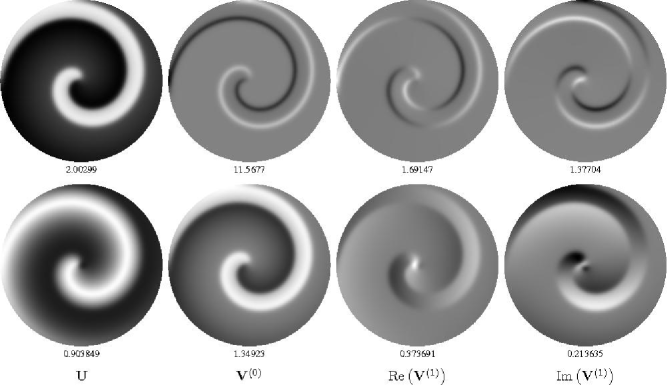
Figure 1: Solutions of the nonlinear problem (3) and the linearized problem (4,5), i.e. the Goldstone modes, at the “best” parameters, $\rho_{\max}=25$, $N_{\rho}=1280$, $N_{\theta}=64$, as density plots. Numbers under the density plots are their amplitudes $A$: white of the plot corresponds to the value $A$ and black corresponds to the value $-A$ of the designated field. Upper row: 1st components, lower row: 2d components.

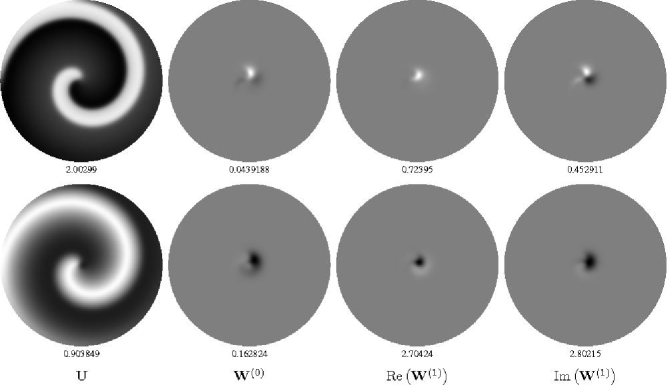
Figure 2: Same visualization as in fig. 1, for the adjoint linearized problem (13,15), i.e. the response functions.

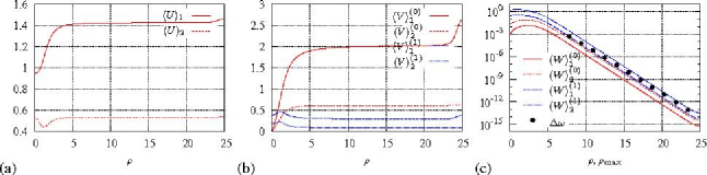
Figure 3: Radial dependence of the angle-averaged solutions for the spiral wave (a), Goldstone modes (b) and response functions (c). In (c), the dependence of $\Delta\omega(\rho_{\max})=\hat{\omega}(\rho_{\max})-\hat{\omega}(25)$ is shown for comparison, where $\hat{\omega}(\rho_{\max})$ is the numerically found spiral angular velocity in the disk of given radius $\rho_{\max}$.

Before discussing the performance of our numerical techniques, we briefly present typical solutions. Figures 1 and 2 illustrate the spiral wave solution and the GMs and RFs for $\rho_{\max}=25$, $N_{\rho}=1280$ and $N_{\theta}=64$. This solution is taken as the best achievable given memory restrictions (4Gb of real memory). The angular velocity for it was found to be $\hat{\omega}\approx 0.5819341748776017$. For the GMs and RFs, we show the $n=0$ and $n=1$ modes only, since the calculated $n=-1$ modes are almost exactly the complex conjugates of the $n=1$ modes, which of course they should be.

One can see that the GMs $\hat{\mathbf{V}}$ are indeed proportional to corresponding derivatives of the spiral wave solution $\hat{\mathbf{U}}$, and that the RFs $\hat{\mathbf{W}}$ are localized in a small region of the spiral tip and are indistinguishable from zero outside that region.

The character of the RFs’ decay with distance is illustrated in more detail in fig. 3. We plot the angle-averaged values of the solutions, defined as

$$\langle{X}\rangle^{(n)}_{i}(\rho)=\frac{1}{2\pi}\oint\hat{X}_{i}^{(n)}(\rho,\theta)\,{\mathrm{d}}\theta,$$

for $X=U,V$ and $W$. Note the difference in the behavior of $\langle{U}\rangle^{(n)}_{i}$ and $\langle{V}\rangle^{(n)}_{i}$ on one hand and $\langle{W}\rangle^{(n)}_{i}$ on the other hand. In the semilogarithmic (linear for horizontal axis, logarithmic for vertical axis) coordinates of fig. 3(c) the graphs of $\langle{W}\rangle^{(n)}_{i}(\rho)$ are straight for a large range of $\rho$, not too close to 0 or $\rho_{\max}=25$, and for several decades of magnitude of $\langle{W}\rangle^{(n)}_{i}$. This shows clearly the expected exponential localization of the RFs. For comparison, we also show convergence of $\hat{\omega}=\hat{\omega}(\rho_{\max})$ in a disk as a function of the disk radius $\rho_{\max}$. Theory Hagan (1982); Biktashev (1989c); Biktasheva and Biktashev (2001); Sandstede (2005) predicts that the $\langle{W}\rangle^{(n)}_{i}(\rho)$ and $\Delta\omega(\rho_{\max})=\hat{\omega}(\rho_{\max})-\hat{\omega}(\infty)$ dependencies should both be decaying exponentials with the same characteristic exponent; this agrees well with the numerical results shown in fig. 3(c).

Sandstede and Scheel Sandstede and Scheel (2000b, 2001) have computed exponential decay/increase rates of eigenfunctions of periodic wavetrains in one spatial dimension. A similar technique should, in principle, also work for the adjoint eigenfunctions. Knowning the asymptotic wavelength of the spiral wave, this can be used to predict the exponential decay rates of the RFs of spiral waves. As can be seen from the results of Wheeler and Barkley Wheeler and Barkley (2006), although such correspondence between 1D and 2D calculations can be established, the accuracy of decay rate estimates for two-dimensional eigenfunctions achieved in this way is insufficient for a meaningful estimate of the accuracy of those eigenfunctions.

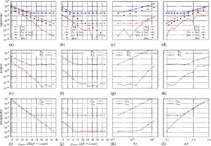
Figure 4: Convergence in numerical parameters: of deviation of the numerical eigenvalues from theoretical (upper row), of $L_{2}$ distance between numerical and theoretical eigenfunctions (second row) and of orthogonality, i.e. Frobenius norm of the difference of the matrix of scalar products of eigenfunctions and adjoint eigenfunctions from the unity matrix (third row), all in logarithmic scales, as dependencies of disk radius (first and second columns, linear scale), radius discretization step (third column, logarithmic scale) and polar angle discretization step (fourth column, logarithmic scale). In the first column, $\rho_{\max}$ is changed while the values of $\Delta\rho$ and $R\Delta\theta$ are kept constant. In the second column, $\rho_{\max}$ is changed while $\Delta\rho$ and $\Delta\theta$ are kept constant.

III.2 Convergence

We now turn to the main results of our study. Convergence of the method has been tested by changing one of the three numerical approximation parameters $\rho_{\max}$, $N_{\rho}$ and $N_{\theta}$ while keeping the other two at the fixed values set by the “best example”. More specifically, while changing $\rho_{\max}$, we consider two variants: one with fixed $N_{\theta}$, and one with changing $N_{\theta}$ so that the combination $\rho_{\max}\Delta\theta$, which is the size of the outermost computational cells in the angular direction, remains constant.

Fig. 4 illustrates the results of the study, where the four columns correspond to different series of calculations, and the three rows correspond to the three different methods of assessing the accuracy: closeness of the eigenvalues to the theoretical values, distance between “numerical” and “analytical” GMs and orthogonality between non-dual RFs and GMs. The scales of $\Delta\rho$, $\Delta\theta$ and the error estimates are logarithmic, and the scales of $\rho_{\max}$ are linear. Here shown is the distance between the “numerical” and “analytical” Goldstone modes in $L_{2}$ norm, the distance in $C_{0}$ norm looks similar.

A typical feature on many of the curves is a “knee”-shape, when the measure of the error decreases as $\rho_{\max}$ grows or $\Delta\theta$ or $\Delta\rho$ decrease, but only until a certain point, beyond which it reaches a plateau. This behavior is expected and explicable. The calculation error is affected by many factors, and if the factor varied in a particular series becomes negligible, then the error remains at a constant level determined by fixed values of other factors.

The position of the “knees” on the curves indicates that the accuracy of the rotational ($n=0$) modes would be improved if $\Delta\theta$ were further decreased (there are no knees on the curves corresponding to the rotational modes, red online, in the fourth, i.e. rightmost column), whereas the limiting parameter for the translational ($n=1$) modes is $\Delta\rho$ (there are no knees on the curves corresponding to the tanslational modes, blue online, in the third column). The analysis of the first two columns is more complicated. The errors estimates at the maximal $\rho_{\max}$ are similar in both columns as they correspond to the same “best” spiral. These limit values are achieved, i.e. plateaux are observed, at much smaller $\rho_{\max}$ values if $\Delta\theta=\mathrm{const}$, than if $\rho_{\max}\Delta\theta=\mathrm{const}$. This is because reduction of $\rho_{\max}$ at fixed $\Delta\theta$ produces an additional improvement of approximation due to the angular discretization. When $\rho_{\max}\Delta\theta$ is kept fixed, as in the first column, the dependence of the solution on the disk radius is without this extra benefit.

The rates of convergence with respect to parameters can be assessed by the slopes of the curves above the knees before they plateau. In some cases the data is somewhat irregular, primarily at parameters corresponding to lower values of error estimates. This is not unexpected and we attribute it to incomplete convergence of the iterative procedures (see below). On the whole, the slopes can be determined clearly from these plots.

The constant slope in the first (leftmost) and the second columns corresponds to the exponential convergence with $\rho_{\max}$. The constant slope in the third column corresponds to power-law convergence, and the typical slope is 2. This is well seen on the curves for translational modes, blue online, and not well on the curves for rotational modes, red online, which are very small anyway. Slope 2 in the third column is to be expected as our discretization is second-order in $\Delta\rho$ in all cases. The curves in the fourth (rightmost) column are convex, which is consistent with the fact that the order of approximation is $N_{\theta}$, which varies along the curve as $\Delta\theta$ varies, since $N_{\theta}=2\pi/\Delta\theta$, so the slope is bigger for smaller $\Delta\theta$. In other words, the high order of the Fornberg approximation of the $\theta$ derivatives implies the convergence in $\Delta\theta$ is faster than any fixed power.

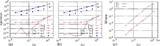
Figure 5: (a,b) Effect of the accuracy of the unperturbed spiral wave solution on the convergence: (a) Newton-iteration tolerance $10^{-8}$. (b) Newton iterations until the norm of the residual stopped decreasing. (c) Convergence of the response functions in $\Delta\rho$.

The irregular shape of some of the curves in fig. 4 at very low values of the error estimates is related to the accuracy of finding the spiral solution and is ulitmately affected by the precision of floating point computations. Note that all calculations in fig. 4 have been performed with a tolerance of $10^{-8}$ for Newton iterations of the spiral wave and some of the curves fall as low as $10^{-15}$ i.e. close to machine epsilon. A change in the tolerance of the Newton iteration reduces irregularities in the curves at low values, as shown in fig. 5(a,b).

Finally, fig. 5(c) illustrates convergence of numerical RFs $\hat{\mathbf{W}}^{(0,1)}$ as $\Delta\rho\to 0$, calculated as the $L_{2}$-distance $\mathcal{E}_{0,1}$ between the solutions at a given resultion $\Delta\rho$ and the “best” solution calculated at the smallest $\Delta\rho_{*}=25/1280$. As explained in the Sec. II.2, this comparsion has been restricted to the series of calculations with varying $\Delta\rho$, where grids at lower resolutions were subgrids of those with higher resolutions. The graphs of $C_{0}$ distances $\mathcal{E}^{\prime}_{0,1}$ looked similar and are not shown here.

IV Discussion

The main result of this paper is a general, robust method for obtaining response functions for rigidly rotating spiral waves in excitable media with required accuracy.

We have tested the method on the FitzHugh-Nagumo model and we have studied the convergence of spiral wave solutions and eigenfunctions, both the Goldstone modes and the response functions, with respect to the numerical approximation parameters $\rho_{\max}$, $N_{\rho}$ and $N_{\theta}$. The rates of convergence are found to agree with the order of approximation and indicate the accuracy with which solutions can be found for particular numerical parameters.

The slowest (second-order) convergence is, as expected, in the parameter $N_{\rho}$. Thus in a typical situation, an improvement of accuracy requires, other things being equal, an increase of $N_{\rho}$, with associated increase in memory and time demands. Thus, the most promising avenue of further development of the method is via increase of the approximation order of the radial derivatives. This is, of course, subject to usual caveat that the degree of approximation should be consistent with the actual smoothness of the solutions.

The method used here to solve the eigenvalue problems for operators $\mathbf{L}$ relies on successive application of transformations of $\mathbf{L}$ applied to a sequence of vectors, alternating with Gram-Schmidt orthogonalization. These are typical ideas, also used in Henry and Hakim (2002); Biktasheva et al. (2006). The difference is that in Henry and Hakim (2002); Biktasheva et al. (2006), the linear transformations were polynomial functions of $\mathbf{L}$ whereas we use rational functions of $\mathbf{L}$. The polynomial iterations used in Henry and Hakim (2002); Biktasheva et al. (2006) were in fact equivalent to solving a Cauchy problem for equation ${\mathrm{d}}{\mathbf{u}}/{\mathrm{d}}{t}=\mathbf{L}\mathbf{u}$ by the explicit Euler method. Therefore, those methods require a large number of iterations, and convergence speed of the iterations depends on the smallness of the absolute difference of the real parts of the eigenvalues of interest compared to those of other eigenvalues. One requires at least $\mathcal{O}(10^{5})$ and typically $\mathcal{O}(10^{6})$ sparse matrix-vector multiplications to achieve the desired solutions to the eigenvalue problem using such an approach.

In contrast, with the complex shift and inversion of $\mathbf{L}$ used in this paper, the convergence speed of the iterations depends on the smallness of the distance of the eigenvalues from their theoretical values used in the complex shift, compared to the distance to other eigenvalues. Hence the number of iterations required is very small, typically $\mathcal{O}(10)$. More specifically, with Krylov subspace dimensionality 3, the number of matrix multiplications with matrix $\mathbf{B}$ of (17) did not exceed 7 per one eigenpair; with Krylov subspace dimensionality 10, this number rose to 10. The price to pay for this acceleration is the necessity to solve large systems of linear equations. However, the key observation is that since the linear system is fixed, it needs to be factorized only once, for a given complex shift, and used for all iterations. Multiplication by matrix $\mathbf{B}$ is achieved with only inexpensive back/forward solves. Moreover, due to the way we ordered the unknowns in the discretized problem, the sparcity of matrix $\mathbf{B}$ does not depend on the order of approximation of $\theta$-derivatives. Hence, we are able to employ high-order approximations requiring far fewer points in the $\theta$ direction for the same accuracy as the second-order finite difference discretization used in Henry and Hakim (2002), thereby further improving the efficiency of our method.

Discounting the factorization step, each iteration, which involves multiplication by $\mathbf{B}$, is comparable to multiplications by $\mathbf{L}$. In practice we find that the factorization itself does not require more than the equivalent of four to six actions of $\mathbf{B}$. On a MacPro with 3 GHz Intel processor, the factorization step takes e.g. about 7.5 sec for the grid $N_{\rho}=1280$, $N_{\theta}=64$, and 0.67 sec for the grid $N_{\rho}=640$, $N_{\theta}=32$; the computation times per $\mathbf{B}$-multiplication were 1.23 sec and 0.17 sec respectively.

The comparison of our present method with Biktasheva et al. (2006) is unequivocal: matrix inverses were not used there, and it was admitted already in Biktasheva et al. (2006) that the resulting accuracy of solutions was severely limited. While direct accuracy and timing comparisons with Henry and Hakim (2002) would be most convincing, that code is not publicly available. However, for reasons already noted, on any given polar grid, the method we report is more accurate due to the angular discretization and considerably faster in floating-point operations.

The computed response functions are localized in the vicinity of the spiral wave tip and exponentially decay with distance from it. This localization ensures convergence of the convolution integral in (12) in an unbounded domain.

The eigenvectors of the linearized operator, i.e. Goldstone modes and of its adjoint, i.e. the response functions have been computed using the same technique, so the qualitatively different behavior of these solutions at large $\rho$ is not a numerical artefact, as it was not in any way assumed in the numerical method.

Although the method has been used here to compute the response functions in the FitzHugh-Nagumo model, none of the details of the method depends on any specifics of the particular reaction kinetics and should be widely applicable to the computation of response functions of rigidly rotating waves in any other model of excitable tissue, as long as its right-hand sides are continuously differentiable so the linarized theory is applicable. Moreover, the method can also be extended in a straightforward way to include additional effects, such as the effect of uniform twist along scroll waves with linear filaments in three dimensions Biktashev (1989b); Margerit and Barkley (2001); Henry and Hakim (2002).

References

- Frisch et al. (1994) T. Frisch, S. Rica, P. Coullet, and J. M. Gilli, Phys. Rev. Lett. 72, 1471 (1994).
- Yu et al. (1999) D. J. Yu, W. P. Lu, and R. G. Harrison, Journal of Optics B — Quantum and Semiclassical Optics 1, 25 (1999).
- Madore and Freedman (1987) B. F. Madore and W. L. Freedman, Am. Sci. 75, 252 (1987).
- Schulman and Seiden (1986) L. S. Schulman and P. E. Seiden, Science 233, 425 (1986).
- Zhabotinsky and Zaikin (1971) A. M. Zhabotinsky and A. N. Zaikin, in Oscillatory processes in biological and chemical systems, edited by E. E. Selkov, A. A. Zhabotinsky, and S. E. Shnol (Nauka, Pushchino, 1971), p. 279, in Russian.
- Jakubith et al. (1990) S. Jakubith, H. H. Rotermund, W. Engel, A. von Oertzen, and G. Ertl, Phys. Rev. Lett. 65, 3013 (1990).
- Agladze and Steinbock (2000) K. Agladze and O. Steinbock, J.Phys.Chem. A 104 (44), 9816 (2000).
- Allessie et al. (1973) M. A. Allessie, F. I. M. Bonk, and F. Schopman, Circ. Res. 33, 54 (1973).
- Gorelova and Bures (1983) N. A. Gorelova and J. Bures, J. Neurobiol. 14, 353 (1983).
- Alcantara and Monk (1974) F. Alcantara and M. Monk, J. Gen. Microbiol. 85, 321 (1974).
- Lechleiter et al. (1991) J. Lechleiter, S. Girard, E. Peralta, and D. Clapham, Science 252 (1991).
- Carey et al. (1978) A. B. Carey, R. H. Giles, Jr., and R. G. Mclean, Am. J. Trop. Med. Hyg. 27, 573 (1978).
- Murray et al. (1986) J. D. Murray, E. A. Stanley, and D. L. Brown, Proc. R. Soc. Lond. ser. B 229, 111 (1986).
- Biktashev (1989a) V. N. Biktashev, Ph.D. thesis, Moscow Institute of Physics and Technology (1989a).
- Biktashev and Holden (1995) V. Biktashev and A. Holden, Chaos, Solitons and Fractals 5, 575 (1995).
- Barkley (1992) D. Barkley, Phys. Rev. Lett. 68, 2090 (1992).
- Biktashev (1989b) V. N. Biktashev, Physica D 36, 167 (1989b).
- Sandstede and Scheel (2000a) B. Sandstede and A. Scheel, Physica D pp. 233–277 (2000a).
- Sandstede and Scheel (2000b) B. Sandstede and A. Scheel, Phys. Rev. E pp. 7708–7714 (2000b).
- Sandstede and Scheel (2001) B. Sandstede and A. Scheel, Phys. Rev. Lett. 86, 171 (2001).
- Wheeler and Barkley (2006) P. Wheeler and D. Barkley, SIAM Journal on Applied Dynamical Systems 5(1), 157 (2006).
- Davydov et al. (1988) V. A. Davydov, V. S. Zykov, A. S. Mikhailov, and P. K. Brazhnik, Izvestia VUZov - Radiofizika 31, 574 (1988), in Russian.
- Zykov (1987) V. S. Zykov, Biofizika 32, 337 (1987), in Russian.
- Keener and Tyson (1990) J. P. Keener and J. J. Tyson, Physica D 44, 191 (1990).
- Keener and Tyson (1991) J. P. Keener and J. J. Tyson, Physica D 53, 151 (1991).
- Davydov et al. (1991) V. A. Davydov, V. S. Zykov, and A. S. Mikhailov, Usp. Fiz. Nauk 161, 45 (1991), in Russian.
- Biktashev and Holden (1994) V. N. Biktashev and A. V. Holden, J. Theor. Biol. 169, 101 (1994).
- Biktashev (1998) V. N. Biktashev, Int. J. of Bifurcation and Chaos 8, 677 (1998).
- Krinsky et al. (1996) V. Krinsky, E. Hamm, and V. Voignier, Phys. Rev. Lett. 76, 3854 (1996).
- Henry (2004) H. Henry, Phys. Rev. E 70, 026204 (2004).
- Keener (1988) J. Keener, Physica D 31, 269 (1988).
- Biktashev et al. (1994) V. N. Biktashev, A. V. Holden, and H. Zhang, Philos. Trans. R. Soc. London ser. A 347, 611 (1994).
- Biktasheva et al. (1998) I. V. Biktasheva, Y. E. Elkin, and V. N. Biktashev, Phys. Rev. E 57, 2656 (1998).
- Biktasheva et al. (1999) I. V. Biktasheva, Y. E. Elkin, and V. N. Biktashev, J. Biol. Phys. 25, 115 (1999).
- Biktasheva (2000) I. V. Biktasheva, Phys. Rev. E 62, 8800 (2000).
- Biktasheva and Biktashev (2001) I. V. Biktasheva and V. N. Biktashev, J. Nonlin. Math. Phys. 8 Supl., 28 (2001).
- Biktasheva and Biktashev (2003) I. V. Biktasheva and V. N. Biktashev, Phys. Rev. E 67, 026221 (2003).
- Sandstede and Scheel (2004) B. Sandstede and A. Scheel, SIAM Journal on Applied Dynamical Systems pp. 1–68 (2004).
- Hamm (1997) E. Hamm, Ph.D. thesis, Université de Nice - Sophia Antipolice / Institut Non Linéair de Nice (1997).
- Henry and Hakim (2002) H. Henry and V. Hakim, Phys. Rev. E 65, 046235 (2002).
- Biktasheva et al. (2006) I. V. Biktasheva, A. V. Holden, and V. N. Biktashev, IJBC 16, 1547 (2006).
- Fornberg (1998) B. Fornberg, A Practical Guide to Pseudospectral Methods (Cambridge University Press, 1998).
- Press et al. (1992) W. Press, B. Flannery, S. Teukolsky, and W. Vetterling, Numerical Recipes in C (Cambridge University Press, Cambridge, UK, 1992).
- Lehoucq et al. (1998) R. B. Lehoucq, D. C. Sorensen, and C. Yang, ARPACK Users’ Guide (SIAM, 1998), ISBN 0898714079, 9780898714074.
- Hagan (1982) P. S. Hagan, SIAM J. Appl. Math. 42, 762 (1982).
- Biktashev (1989c) V. N. Biktashev, in Nonlinear Waves II. Dynamics and evolution, edited by A. V. Gaponov-Grekhov, M. I. Rabinovich, and J. Engelbrecht (Springer, Berlin, 1989c), pp. 87–96.
- Sandstede (2005) B. Sandstede, private communication (2005).
- Margerit and Barkley (2001) D. Margerit and D. Barkley, Phys. Rev. Lett. 86, 175 (2001).