The hyperfine energy levels of alkali metal dimers:
ground-state homonuclear molecules in magnetic fields

Abstract

We investigate the hyperfine energy levels and Zeeman splittings for homonuclear alkali-metal dimers in low-lying rotational and vibrational states, which are important for experiments designed to produce quantum gases of deeply bound molecules. We carry out density-functional theory (DFT) calculations of the nuclear hyperfine coupling constants. For nonrotating states, the zero-field splittings are determined almost entirely by the scalar nuclear spin-spin coupling constant. By contrast with the heteronuclear case, the total nuclear spin remains a good quantum number in a magnetic field. We also investigate levels with rotational quantum number $N=1$, which have long-range anisotropic quadrupole-quadrupole interactions and may be collisionally stable. For these states the splitting is dominated by nuclear quadrupole coupling for most of the alkali-metal dimers and the Zeeman splittings are considerably more complicated.

I Introduction

There have been enormous advances over the last year in experimental methods to produce ultracold molecules in their rovibrational ground state at microkelvin temperatures. Ospelkaus et al. Ospelkaus:2008 produced KRb molecules in high-lying states by magnetoassociation (Feshbach resonance tuning) and then transferred them by stimulated Raman adiabatic passage to levels of the ${}^{1}\Sigma^{+}$ ground state bound by more than 10 GHz. This was then extended by Ni et al. Ni:KRb:2008 to produce molecules in $(v,N)=(0,0)$, where $v$ and $N$ are the quantum numbers for molecular vibration and mechanical rotation. Danzl et al. Danzl:v73:2008 ; Danzl:ground:2008 have carried out analogous experiments on Cs dimers, while Lang et al. Lang:cruising:2008 ; Lang:ground:2008 have produced Rb₂ molecules in the lowest rovibrational level of the lowest triplet state. There have also been considerable successes in direct photoassociation to produce low-lying states Sage:2005 ; Hudson:PRL:2008 ; Viteau:2008 ; Deiglmayr:2008 .

A major goal of the experimental work is to produce a stable molecular quantum gas. However, such a gas can form only if (i) a large number of molecules are in the same hyperfine state and (ii) the molecules are stable to collisions that occur in the gas. In particular, inelastic collisions that transfer internal energy into relative translational energy cause heating and/or trap loss. It is thus very important to understand the hyperfine structure of the low-lying levels and its dependence on applied electric and magnetic fields. In a previous paper, we explored the hyperfine levels of heteronuclear alkali metal dimers in rotationless levels Aldegunde:polar:2008 . The purpose of the present paper is to extend this work to homonuclear molecules, which have important special features. We also explore $N=1$ levels, which may be collisionally stable for homonuclear molecules and which interact with longer-range forces than $N=0$ levels.

II Molecular Hamiltonian

The Hamiltonian of a diatomic molecule in the presence of an external magnetic field can be decomposed into five different contributions: the electronic, vibrational, rotational, hyperfine and Zeeman terms. For ${}^{1}{\rm\Sigma}$ molecules in a fixed vibrational level, the first two terms take a constant value and the rotational, hyperfine and Zeeman parts of the Hamiltonian may be written Ramsey:1952 ; Brown ; Bryce:2003

$$H=H_{\rm rot}+H_{\rm hf}+H_{\rm Z},$$ (1)

where

$$H_{\rm rot} = B_{v}\bm{N}^{2}-D_{v}\bm{N}^{2}\cdot\bm{N}^{2};$$ (2)

$$H_{\rm hf} = H_{\rm Q}+H_{\rm IN}+H_{\rm t}+H_{\rm sc}=\sum_{i=1}^{2}\bm{V}_{i}:\bm{Q}_{i}$$ (3)

$$+ \sum_{i=1}^{2}c_{i}\,\bm{N}\cdot\bm{I}_{i}+c_{3}\,\bm{I}_{1}\cdot\bm{T}\cdot\bm{I}_{2}+c_{4}\,\bm{I}_{1}\cdot\bm{I}_{2};$$

$$H_{\rm Z} = -g_{\rm r}\mu_{\rm N}\,\bm{N}\cdot\bm{B}-\sum_{i=1}^{2}g_{i}\mu_{\rm N}\,\bm{I}_{i}\cdot\bm{B}(1-\sigma_{i}).$$ (4)

where the index $i$ refers to each of the nuclei in the molecule. $\bm{N}$, $\bm{I}_{1}$ and $\bm{I}_{2}$ represent the operators for mechanical rotation and for the spins of nuclei 1 and 2. The rotational and centrifugal constants of the molecule are given by $B_{v}$ and $D_{v}$ (but centrifugal distortion is neglected in the present work). We use $\bm{N}$ rather than $\bm{J}$ for mechanical rotation because we wish to reserve $\bm{J}$ for the angular momentum including electron spin for future work on triplet states.

The hyperfine Hamiltonian of equation 3 consists of four different contributions. The first is the electric quadrupole interaction $H_{\rm Q}$, with coupling constants $(eqQ)_{1}$ and $(eqQ)_{2}$. It represents the interaction of the nuclear quadrupoles ($eQ_{i}$) with the electric field gradients $q_{i}$ created by the electrons at the nuclear positions. The second is the spin-rotation term $H_{\rm IN}$, which describes the interaction of the nuclear magnetic moments with the magnetic moment created by the rotation of the molecule. Its coupling constants are $c_{1}$ and $c_{2}$. For a homonuclear molecule with identical nuclei, $(eqQ)_{1}=(eqQ)_{2}$ and $c_{1}=c_{2}$. The last two terms represent the interaction between the two nuclear spins; there is both a tensor component $H_{\rm t}$, with coupling constant $c_{3}$, and a scalar component $H_{\rm sc}$, with coupling constant $c_{4}$. The second-rank tensor $\bm{T}$ represents the angular part of a dipole-dipole interaction.

The Zeeman Hamiltonian $H_{\rm Z}$ has both rotational and nuclear Zeeman contributions characterized by $g$-factors $g_{\rm r}$, $g_{1}$ and $g_{2}$. For homonuclear molecules $g_{1}=g_{2}$. The nuclear shielding tensor ${\bm{\sigma}}_{i}$ is approximated here by its isotropic part $\sigma_{i}$; terms involving the anisotropy of ${\bm{\sigma}}_{i}$ are extremely small for the states considered here.

The nuclear $g$-factors and the quadrupole moments of the nuclei are experimentally known Stone:2005 .

For homonuclear molecules we neglect the effect of electric fields, though in principle there are small effects due to anisotropic polarizabilities and the molecular quadrupole moments can interact with the gradients of inhomogeneous fields.

III Evaluation of the coupling constants

The rotational $g$-factors are known experimentally for all the homonuclear alkali metal dimers Brooks:1963 . However, the only such species for which the nuclear hyperfine coupling constants have been determined accurately is Na₂ Esbroeck:1985 . We have therefore evaluated the remaining coupling constants using density-functional theory (DFT) calculations performed with the Amsterdam density functional (ADF) package ADF1 ; ADF3 with all-electron basis sets and including relativistic corrections. A full description of the basis sets, functionals, etc. used in the calculations has been given in our previous paper on heteronuclear systems Aldegunde:polar:2008 . In the present work, the calculations were carried out at the equilibrium geometries ($R_{e}=2.67$ Å for Li₂ Hessel:1979 , 3.08 Å for Na₂ Kusch:1978 , 3.92 Å for K₂ Engelke:1984 , 4.21 Å for Rb₂ Amiot:1985 and 4.65 Å for Cs₂ Raab:1982 ). This give results that are approximately valid not only for $v=0$ states but also for other low-lying vibrational states.

The values for the coupling constants are given in table 1. It may be seen that the DFT results for Na₂ are within about 30% of the experimental values, and similar accuracy was obtained for other test cases in our previous work Aldegunde:polar:2008 . The accuracy is likely to be comparable for the other cases studied here. This level of accuracy is adequate for the purpose of the present paper, which aims to explore the qualitative nature of the Zeeman patterns. Most of our conclusions are insensitive to the exact magnitudes of the coupling constants.

Table 1: Nuclear quadrupole moment ($Q$), electric quadrupole coupling constant ($eqQ$), nuclear $g$-factor ($g$), spin-rotation coupling constant ($c_{1}$), tensor spin-spin coupling constant ($c_{3}$), scalar spin-spin coupling constant ($c_{4}$), absolute value of the $c_{4}/(eqQ)$ ratio, isotropic part of the nuclear shielding ($\sigma$) and rotational $g$-factor ($g_{\rm{r}}$) for the homonuclear alkali dimers. All the quantities except the nuclear quadrupole moments, the nuclear g-factors and the rotational g-factors were evaluated using DFT calculations (see section III). Both experimental Esbroeck:1985 and theoretical results are presented for Na₂.

	$Q$(fm2)	$eqQ$(MHz)	$g$	$c_{1}$(Hz)	$c_{3}$(Hz)	$c_{4}$(Hz)	$|c_{4}/(eqQ)|$	$\sigma$(ppm)	$g_{\rm{r}}$
6Li2	-0.082	0.00123	0.822	161	137	32	0.026	102	0.1259
7Li2	-4.06	0.0608	2.171	365	955	226	0.0037	102	0.1080
23Na2 (Exp.)	10.45	-0.459	1.479	243	303	1067	0.0023	—	0.0386
23Na2 (DFT)	—	-0.456	—	299	298	1358	0.0030	613	—
39K2	5.85	-0.290	0.261	35	5	106	0.00036	1313	0.0212
40K2	-7.3	0.362	-0.324	-42	8	163	0.00045	1313	0.0207
41K2	7.11	-0.353	0.143	18	2	32	0.000091	1313	0.0202
85Rb2	27.7	-2.457	0.541	63	30	2177	0.00089	3489	0.0095
87Rb2	13.4	-1.188	1.834	209	346	25021	0.021	3489	0.0093
${}^{133}{\rm Cs}_{2}$	-0.355	0.0486	0.738	96	119	12993	0.27	6461	0.0054

IV Hyperfine energy levels

Our previous work Aldegunde:polar:2008 showed that the zero-field splitting for heteronuclear diatomic molecules in $N=0$ states is determined almost entirely by the scalar nuclear spin-spin interaction. This remains true for homonuclear molecules in $N=0$ states. We show below that for $N>0$ the electric quadrupole interaction is dominant for all the homonuclear dimers except Cs₂ and ⁶Li₂, with smaller but significant contributions from the remaining coupling constants.

For all systems except Li₂, the scalar spin-spin coupling is considerably stronger than the spin-rotation and tensor spin-spin couplings. Knowledge of the nuclear quadrupole coupling constant $eQq$ and the scalar spin-spin coupling constant $c_{4}$ is therefore sufficient to understand the hyperfine splitting patterns. We will focus here on ⁸⁵Rb₂ and ⁸⁷Rb₂, which form a convenient pair that approximately cover the range of values of the ratio $|c_{4}/(eqQ)|$. Lang et al. Lang:ground:2008 have produced ⁸⁷Rb₂ in the lowest rovibrational level of the lowest triplet state, but as far as we are aware not yet in the singlet state.

The hyperfine energy levels are obtained by diagonalizing the matrix representation of the Hamiltonian (1) in a basis set of angular momentum functions. In order to facilitate the assignment of quantum numbers to the energy levels, two different basis sets are employed,

$$|(I_{1}I_{1})IM_{I}NM_{N}\rangle (\mbox{spin-coupled basis});$$ (5)

$$|(I_{1}I_{1})INFM_{F}\rangle (\mbox{fully coupled basis}).$$ (6)

where $I$ and $F$ are the total nuclear spin and total angular momentum quantum numbers and $M_{I}$ and $M_{F}$ are their projections onto the $Z$ axis defined by the external field. The matrix elements of the different terms in the Hamiltonian in each of the basis sets are calculated through standard angular momentum techniques Zare . Explicit expressions are given in the Appendix.

For homonuclear molecules, nuclear exchange symmetry dictates that not all possible values of the total nuclear spin $I$ can exist for each rotational level. For molecules in ${}^{1}\Sigma^{+}$ states, only even $I$ values can exist for even $N$ and only odd $I$ for odd $N$. This is true for either fermionic or bosonic nuclei but is reversed for ${}^{3}\Sigma^{+}$ states. Table 2 summarizes the $I$-$N$ pairs compatible with the antisymmetry of the wave function under nuclear exchange for the Rb₂ isotopomers.

Table 2: Values of $I$ permitted by the nuclear exchange symmetry for even and odd rotational levels of ⁸⁵Rb₂ and ⁸⁷Rb₂.

		$N$		$I$
		even		0, 2, 4
85Rb2($I_{\rm{Rb}}=5/2$)		odd		1, 3, 5
		even		0, 2
87Rb2($I_{\rm{Rb}}=3/2$)		odd		1, 3

IV.1 Zeeman splitting for $N=0$ homonuclear alkali dimers

The Zeeman splittings for the $N=0$ hyperfine levels of ⁸⁵Rb₂ and ⁸⁷Rb₂ are shown in figure 1. The zero-field splittings are in most respects similar to those found for heteronuclear molecules in the ground rotational state Aldegunde:polar:2008 . The similarities can be summarized as follows:

• The scalar nuclear spin-spin interaction and the nuclear Zeeman effect are the only two terms in the molecular Hamiltonian with nonzero diagonal elements for $N=0$.

• The electric quadrupole and the tensor nuclear spin-spin interactions are not diagonal in $N$, coupling the $N$, $N+2$ and $N-2$ rotational levels. This means that the energy levels should be converged by including in the calculations as many rotational levels as necessary. However, the coupling constants $eQq$ and $c_{3}$ are very much smaller than the rotational spacings, so that in practice it is adequate to include one excited rotational level. Convergence for $N=0$ is reached with $N_{\rm max}=2$ and convergence for $N=1$ is reached with $N_{\rm max}=3$.

• The scalar spin-spin interaction is diagonal in both the spin-coupled and fully coupled basis sets, which for $N=0$ are identical,

  $$\langle(N=0)IM_{I}|c_{4}\,\bm{I}_{1}\cdot\bm{I}_{2}|(N=0)IM_{I}\rangle$$

  $$\qquad=\frac{1}{2}c_{4}[I(I+1)-2I_{\rm Rb}(I_{\rm Rb}+1)].$$ (7)

  Except for a very small contribution coming from the coupling with $N=2$ levels, these diagonal elements determine the zero-field splitting.

Figure 1: Zeeman splitting of hyperfine levels for $N=0$ states of ⁸⁵Rb₂ (upper panel) and ⁸⁷Rb₂ (lower panel).

Despite the similarity of the zero-field levels, there are important differences between the Zeeman splittings for heteronuclear and homonuclear molecules. For heteronuclear dimers Aldegunde:polar:2008 , levels with the same $M_{I}$ but different $I$ exhibit avoided crossings as a function of magnetic field. Because of this, $I$ is no longer a good quantum number at high field but the individual nuclear spin projections $M_{I1}$ and $M_{I_{2}}$ become nearly conserved. For homonuclear dimers, however, different energy levels that correspond to the same value of $M_{I}$ are parallel, so that no avoided crossings appear as a function of the field. Both $I$ and $M_{I}$ remain good quantum numbers regardless of the value of the magnetic field but $M_{I1}$ and $M_{I_{2}}$ are not individually conserved. This is illustrated in figure 1. It arises because the nuclear Zeeman term, which is the only nondiagonal term for $N=0$ in the heteronuclear case, is diagonal for homonuclear molecules. Its nonzero elements are given by equation 75 of the Appendix,

$$\langle(N=0)IM_{I}|H_{\rm IZ}|(N=0)IM_{I}\rangle$$

$$\qquad=-g_{\rm Rb}\mu_{\rm N}B_{\rm Z}(1-\sigma_{\rm Rb})M_{I}.$$ (8)

The nuclear Zeeman term is diagonal because the $g$-factors of the two nuclei are equal and not because of nuclear exchange symmetry. The $N=0$ block of the molecular Hamiltonian for a heteronuclear dimer with two identical nuclear $g$-factors would also be diagonal.

The conservation of the total nuclear spin $I$ and non-conservation of $M_{I1}$ and $M_{I2}$ at high fields may have important consequences for the selection rules in spectroscopic transitions used to produce ultracold molecules and for the collisional stability of molecules in excited hyperfine states.

IV.2 Zeeman splitting for $N=1$ homonuclear alkali dimers

Ultracold homonuclear molecules in $N=1$ states are particularly interesting because they are likely to be stable with respect to inelastic collisions to produce $N=0$, at least for collisions with non-magnetic species such as other molecules in ${}^{1}\Sigma$ states. Such collisions cannot change the nuclear spin symmetry and thus cannot change $N$ from odd to even. Inelastic collisions may well be stronger for collisions of molecules in triplet states, because of magnetic interactions between electron and nuclear spins. Transitions between odd and even rotational levels are permitted in atom-exchange collisions, such as occur in collisions with alkali metal atoms Soldan:2002 ; Cvitas:bosefermi:2005 ; Cvitas:hetero:2005 ; Quemener:2005 ; Cvitas:li3:2007 ; Hutson:IRPC:2007 .

Homonuclear molecules do not possess electric dipole moments but do have quadrupole moments. The quadrupole-quadrupole interaction is anisotropic and is proportional to $R^{-5}$, so is longer-range than the $R^{-6}$ dispersion interaction that acts between neutral atoms and molecules. The quadrupole-quadrupole interaction averages to zero for rotationless states ($N=0$), but not for $N>0$. Quantum gases of rotating homonuclear molecules may thus exhibit anisotropic effects.

For $N>0$, all the terms in the Hamiltonian (1) have matrix elements diagonal in $N$. Some of these are nondiagonal in hyperfine quantum numbers, so the energy level patterns are much more intricate. The zero-field splitting is dominated in most cases by the electric quadrupole interaction and the scalar nuclear spin-spin term. The remaining constants ($c_{1}$ and $c_{3}$) make much smaller contributions except for the two Li₂ isotopomers. For ⁶Li₂, all the terms in the hyperfine hamiltonian contribute significantly. For ⁷Li₂, the splitting is dominated by the electric quadrupole interaction but contributions from all the remaining terms are significant.

Figure 2 shows the “building-up” of the zero-field $N=1$ hyperfine energy levels for ⁸⁵Rb₂ and ⁸⁷Rb₂ in three steps: first, only the rotational and the electric quadrupole terms are considered; secondly, the scalar spin-spin interaction is included; and thirdly, the spin-rotation and the tensor spin-spin interaction terms are added to complete the hyperfine Hamiltonian. For ⁸⁵Rb₂, the electric quadrupole term alone determines the energy level pattern, while for ⁸⁷Rb₂ there is a significant additional contribution from the scalar spin-spin interaction, attributable to the relatively large value of $c_{4}$ for this molecule (see table 1).

Figure 2: Zero-field hyperfine splitting for $N=1$ states of ⁸⁵Rb₂ (upper panel) and ⁸⁷Rb₂ (lower panel). For each species, the hyperfine energy levels obtained when only the rotational and electric quadrupole terms are included are show in the left column. The effect of adding the scalar spin-spin interaction is displayed in the central column and, finally, the right column shows the splitting when the whole hyperfine Hamiltonian is considered. All the energies are referred to the lowest hyperfine level for the complete Hamiltonian.

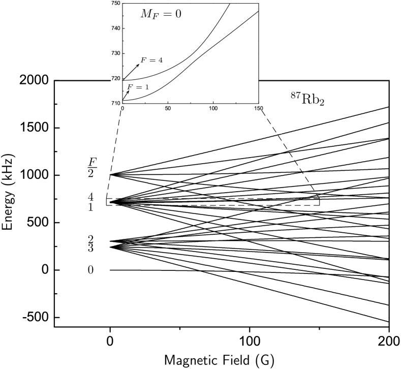
Figure 3: Zeeman splitting for $N=1$ states of ⁸⁵Rb₂ (upper panel) and ⁸⁷Rb₂ (lower panel). The inset for ⁸⁷Rb₂ shows the avoided crossing of $M_{F}=0$ states.

Figure 4: Zeeman splitting for $N=1$ states of ⁸⁵Rb₂. The avoided crossings for $M_{F}=0$ are shown in the lower panel.

The quantum numbers that label the zero-field energy levels are included in figure 2. The total angular momentum quantum number $F$ is always a good quantum number at zero field. In some cases, when there is only one pair of values $I$ and $N$ that can couple to give the resultant $F$, $I$ is also a good quantum number. Otherwise, $I$ is mixed and the values given in figure 2 are ordered according to their contribution to the eigenstate: the first quantum number listed identifies the largest contribution.

The Zeeman splittings for $N=1$ states of ⁸⁵Rb₂ and ⁸⁷Rb₂ for different ranges of magnetic fields are shown in figures 3 and 4. Each zero-field level splits into $2F+1$ states with different projection quantum numbers $M_{F}$. Although in principle both the nuclear ($H_{\rm IZ}$) and the rotational ($H_{\rm NZ}$) Zeeman terms contribute to the splitting, $g_{\rm Rb}\gg g_{\rm r}$ so that the rotational Zeeman term contributes only about 1% for ⁸⁵Rb₂ and less than 0.5% for ⁸⁷Rb₂.

In contrast with the $N=0$ case, the Hamiltonian for $N=1$ is not diagonal and energy levels corresponding to the same $M_{F}$ value display avoided crossings. The magnetic field values at which the avoided crossings are found, between 0 and 2000 G for ⁸⁵Rb₂ (lower panel of figure 4) and between 0 and 200 G for ⁸⁷Rb₂ (lower panel of figure 3), scale with the ratio between the electric quadrupole constant and the nuclear $g$-factor.

For larger magnetic fields, $M_{I}$ and $M_{N}$ become individually good quantum numbers and the energy levels corresponding to the same value of $M_{I}$ gather together. Both features are illustrated in figure 4 where, for the sake of clarity, the values of $M_{N}$ are included only in the lower panel. Equation 75 shows that the matrix representation of the nuclear Zeeman term in the spin-coupled basis is diagonal with nonzero elements proportional to $M_{I}$ and independent of any other quantum number. As the magnetic field increases the nuclear Zeeman terms becomes dominant and the slope of the energy levels is determined by $M_{I}$.

The results in figure 4 neglect the diamagnetic Zeeman interaction, which is not completely negligible at the highest fields considered (up to 4000 G). The justification for this is as follows. The Hamiltonian for the diamagnetic Zeeman interaction Ramsey:1952 consists of two terms proportional to the square of the magnetic field: one depending on the trace of the magnetizability tensor and the other is proportional to its anisotropic part. The first term has a value around 200 kHz at 4000 G for ⁸⁵Rb₂. Although this quantity is not negligible, it has not been included because it simply shifts all the energy levels by the same amount and has no effect on splittings. The second term is diagonal in the spin-coupled basis set and its nonzero elements depend on $N$ and $M_{N}$. For ⁸⁵Rb₂ at 4000 G it would shift the energy levels by about 15 kHz. It is therefore very small compared to the nuclear Zeeman effect.

V Conclusions

We have explored the hyperfine energy levels and Zeeman splitting patterns for low-lying rovibrational states of homonuclear alkali-metal dimers in ${}^{1}\Sigma$ states. We have calculated the nuclear hyperfine coupling constants for all common isotopic species of the homonuclear dimers from Li₂ to Cs₂ and explored the energy level patterns in detail for ⁸⁵Rb₂ and ⁸⁷Rb₂.

For rotationless molecules ($N=0$ states), the zero-field splitting arises almost entirely from the scalar nuclear spin-spin coupling. The levels are characterized by a total nuclear spin quantum number $I$ and states with different values of $I$ are separated by amounts between 90 Hz for ⁴¹K₂ and 160 kHz for ¹³³Cs₂. When a magnetic field is applied, each level splits into $2I+1$ components but all the levels with a particular value of $M_{I}$ are parallel. This is different from the heteronuclear case, and for homonuclear molecules $I$ remains a good quantum number in a magnetic field. However, the projection quantum numbers $M_{I1}$ and $M_{I2}$ for individual nuclei do not become nearly good quantum numbers at high fields for homonuclear molecules. These differences in quantum numbers may have important consequences for spectroscopic selection rules and for the collisional stability of molecules in excited hyperfine states.

Molecules in excited rotational states are also of considerable interest. In particular, molecules in $N=1$ states may be collisionally stable because transitions between even and odd rotational levels require a change in nuclear exchange symmetry. Molecules in excited rotational states have anisotropic quadrupole-quadrupole interactions that are longer-range than dispersion interactions. The hyperfine energy level patterns are considerably more complicated for $N=1$ states than for $N=0$ states and $I$ is not in general a good quantum number even at zero field.

The results of the present paper will be important in studies that produce ultracold molecules in low-lying rovibrational levels, where it is important to understand and control the population of molecules in different hyperfine states.

Appendix A A

Explicit expressions for the matrix elements of the molecular Hamiltonian terms are now provided. The equations are valid for homonuclear molecules.

The matrix elements for the rotational term ($H_{\rm rot}$) are given by

$$\langle NM_{N}(I_{\rm 1}I_{\rm 1})IM_{I}|H_{\rm rot}|N^{\prime}M_{N^{\prime}}(I_{\rm 1}I_{\rm 1})I^{\prime}M_{I^{\prime}}\rangle = \delta_{NN^{\prime}}\,\delta_{M_{N}M_{N^{\prime}}}\,\delta_{II^{\prime}}\,\delta_{M_{I}M_{I^{\prime}}}B\,N(N+1)$$ (9)

$$\langle N(I_{\rm 1}I_{\rm 1})IFM_{F}|H_{\rm sc}|N^{\prime}(I_{\rm 1}I_{\rm 1})I^{\prime}F^{\prime}M_{F^{\prime}}\rangle = \delta_{NN^{\prime}}\,\delta_{II^{\prime}}\,\delta_{FF^{\prime}}\,\delta_{M_{F}M_{\rm F^{\prime}}}B\,N(N+1).$$ (10)

The matrix elements for the electric quadrupole interaction ($H_{\rm Q}$) are given by

$$\langle NM_{N}(I_{\rm 1}I_{\rm 1})IM_{I}| H_{\rm Q} |N^{\prime}M_{N^{\prime}}(I_{\rm 1}I_{\rm 1})I^{\prime}M_{I^{\prime}}\rangle=\frac{(eqQ)_{1}}{4}\,(-1)^{2I_{1}}\{4(2N+1)(2N^{\prime}+1)(2I+1)(2I^{\prime}+1)\}^{1/2}$$ (17)

$$\times \left(\begin{array}[]{ccc}N&2&N^{\prime}\\ 0&0&0\end{array}\right)\left(\begin{array}[]{ccc}I_{1}&2&I_{1}\\ -I_{1}&0&I_{1}\end{array}\right)^{-1}\left\{\begin{array}[]{ccc}I_{1}&I&I_{1}\\ I^{\prime}&I_{1}&2\end{array}\right\}$$

$$\times \sum_{FM_{F}}\Bigg{[}(-1)^{F+2M_{F}}(2F+1)\left(\begin{array}[]{ccc}N&I&F\\ M_{N}&M_{I}&-M_{F}\end{array}\right)$$ (20)

$$\times \left(\begin{array}[]{ccc}N^{\prime}&I^{\prime}&F\\ M_{N^{\prime}}&M_{I^{\prime}}&-M_{F}\end{array}\right)\left\{\begin{array}[]{ccc}I&N&F\\ N^{\prime}&I^{\prime}&2\end{array}\right\}\Bigg{]}$$ (25)

$$\langle N(I_{\rm 1}I_{\rm 1})IFM_{F}| H_{\rm Q} |N^{\prime}(I_{\rm 1}I_{\rm 1})I^{\prime}F^{\prime}M_{F^{\prime}}\rangle=\delta_{FF^{\prime}}\,\delta_{M_{F}M_{\rm F^{\prime}}}\frac{(eqQ)_{1}}{4}\,(-1)^{N+N^{\prime}+F+2I_{1}}\{4(2N+1)(2N^{\prime}+1)\}^{1/2}$$ (34)

$$\times \{(2I+1)(2I^{\prime}+1)\}^{1/2}\left(\begin{array}[]{ccc}N&2&N^{\prime}\\ 0&0&0\end{array}\right)\left(\begin{array}[]{ccc}I_{1}&2&I_{1}\\ -I_{1}&0&I_{1}\end{array}\right)^{-1}\left\{\begin{array}[]{ccc}I&N&F\\ N^{\prime}&I^{\prime}&2\end{array}\right\}\left\{\begin{array}[]{ccc}I_{1}&I&I_{1}\\ I^{\prime}&I_{1}&2\end{array}\right\}$$

The matrix elements for the spin-rotation interaction ($H_{\rm IJ}$) are given by

$$\langle NM_{N}(I_{\rm 1}I_{\rm 1})IM_{I}| H_{\rm IJ} |N^{\prime}M_{N^{\prime}}(I_{\rm 1}I_{\rm 1})I^{\prime}M_{I^{\prime}}\rangle=\delta_{NN^{\prime}}\delta_{II^{\prime}}c_{1}(-1)^{N-M_{N}-M_{I}+2I_{1}+1}2(2I+1)$$ (37)

$$\times \{(2N+1)N(N+1)(2I_{1}+1)I_{1}(I_{1}+1)\}^{1/2}\left\{\begin{array}[]{ccc}I_{1}&I&I_{1}\\ I&I_{1}&1\end{array}\right\}$$

$$\times \sum_{p}\Bigg{[}(-1)^{p}\left(\begin{array}[]{ccc}N&1&N\\ -M_{N}&p&M_{N^{\prime}}\end{array}\right)\left(\begin{array}[]{ccc}I&1&I\\ -M_{I}&-p&M_{I^{\prime}}\end{array}\right)\Bigg{]}$$ (42)

$$\langle N(I_{\rm 1}I_{\rm 1})IFM_{F}| H_{\rm IJ} |N^{\prime}(I_{\rm 1}I_{\rm 1})I^{\prime}F^{\prime}M_{F^{\prime}}\rangle=-2\delta_{NN^{\prime}}\,\delta_{II^{\prime}}\,\delta_{FF^{\prime}}\,\delta_{M_{F}M_{\rm F^{\prime}}}c_{1}(-1)^{F+2I_{1}-M_{F}-I}(2F+1)$$ (45)

$$\times (2I+1)\{(2N+1)N(N+1)(2I_{1}+1)I_{1}(I_{1}+1)\}^{1/2}\left\{\begin{array}[]{ccc}I_{1}&I&I_{1}\\ I&I_{1}&1\end{array}\right\}$$

$$\times \sum_{F^{\prime\prime},M_{\rm F^{\prime\prime}}}\Bigg{[}(-1)^{F^{\prime\prime}+M_{\rm F^{\prime\prime}}}(2F^{\prime\prime}+1)\left\{\begin{array}[]{ccc}N&F&I\\ F^{\prime\prime}&N&1\end{array}\right\}$$ (48)

$$\times \sum_{p}\bigg{[}(-1)^{p}\left(\begin{array}[]{ccc}F&1&F^{\prime\prime}\\ -M_{F}&p&M_{\rm F^{\prime\prime}}\end{array}\right)^{2}\bigg{]}\left\{\begin{array}[]{ccc}I&F^{\prime\prime}&N\\ F&I&1\end{array}\right\}\Bigg{]}$$ (53)

The matrix elements for the scalar nuclear spin-spin interaction ($H_{\rm sc}$) are given by

$$\langle NM_{N}(I_{\rm 1}I_{\rm 1})IM_{I}|H_{\rm sc}|N^{\prime}M_{N^{\prime}}(I_{\rm 1}I_{\rm 1})I^{\prime}M_{I^{\prime}}\rangle = \delta_{NN^{\prime}}\delta_{M_{N}M_{N^{\prime}}}\delta_{II^{\prime}}\delta_{M_{I}M_{I^{\prime}}}\frac{1}{2}c_{4}[I(I+1)-2I_{\rm 1}(I_{\rm 1}+1)]$$ (54)

$$\langle N(I_{\rm 1}I_{\rm 1})IFM_{F}|H_{\rm sc}|N^{\prime}(I_{\rm 1}I_{\rm 1})I^{\prime}F^{\prime}M_{F^{\prime}}\rangle = \delta_{NN^{\prime}}\,\delta_{II^{\prime}}\,\delta_{FF^{\prime}}\,\delta_{M_{F}M_{\rm F^{\prime}}}\frac{1}{2}c_{4}[I(I+1)-2I_{\rm 1}(I_{\rm 1}+1)]$$ (55)

The matrix elements for the tensor nuclear spin-spin interaction ($H_{\rm t}$) are given by

$$\langle NM_{N}(I_{\rm 1}I_{\rm 1})IM_{I}| H_{\rm t} |N^{\prime}M_{N^{\prime}}(I_{\rm 1}I_{\rm 1})I^{\prime}M_{I^{\prime}}\rangle=-c_{3}\sqrt{30}(-1)^{I-M_{I}-M_{N}}I_{1}(I_{1}+1)(2I_{1}+1)\{(2N+1)(2N^{\prime}+1)\}^{1/2}$$ (61)

$$\times \{(2I+1)(2I^{\prime}+1)\}^{1/2}\left(\begin{array}[]{ccc}N&2&N^{\prime}\\ 0&0&0\end{array}\right)\left\{\begin{array}[]{ccc}I_{1}&I_{1}&1\\ I_{1}&I_{1}&1\\ I&I^{\prime}&2\end{array}\right\}$$

$$\times \sum_{p}\Bigg{[}(-1)^{p}\left(\begin{array}[]{ccc}N&2&N^{\prime}\\ -M_{N}&p&M_{N^{\prime}}\end{array}\right)\left(\begin{array}[]{ccc}I&2&I^{\prime}\\ -M_{I}&-p&M_{I^{\prime}}\end{array}\right)\Bigg{]}$$ (66)

$$\langle N(I_{\rm 1}I_{\rm 1})IFM_{F}| H_{\rm t} |N^{\prime}(I_{\rm 1}I_{\rm 1})I^{\prime}F^{\prime}M_{F^{\prime}}\rangle=-\delta_{FF^{\prime}}\,\delta_{M_{F}M_{\rm F^{\prime}}}c_{3}\sqrt{30}(-1)^{N^{\prime}+N+I+F}I_{1}(I_{1}+1)(2I_{1}+1)$$ (74)

$$\times \{(2N+1)(2N^{\prime}+1)(2I+1)(2I^{\prime}+1)\}^{1/2}\left(\begin{array}[]{ccc}N&2&N^{\prime}\\ 0&0&0\end{array}\right)\left\{\begin{array}[]{ccc}N&I&F\\ I^{\prime}&N^{\prime}&2\end{array}\right\}\left\{\begin{array}[]{ccc}I_{1}&I_{1}&1\\ I_{1}&I_{1}&1\\ I&I^{\prime}&2\end{array}\right\}$$

The matrix elements for the nuclear Zeeman term ($H_{\rm IZ}$) are given by

$$\langle NM_{N}(I_{\rm 1}I_{\rm 1})IM_{I}| H_{\rm IZ} |N^{\prime}M_{N^{\prime}}(I_{\rm 1}I_{\rm 1})I^{\prime}M_{I^{\prime}}\rangle=-\delta_{NN^{\prime}}\delta_{M_{N}M_{N^{\prime}}}\delta_{II^{\prime}}\delta_{M_{I}M_{I^{\prime}}}g_{1}\mu_{\rm N}B_{\rm Z}(1-\sigma_{1})M_{I}$$ (75)

$$\langle N(I_{\rm 1}I_{\rm 1})IFM_{F}| H_{\rm IZ} |N^{\prime}(I_{\rm 1}I_{\rm 1})I^{\prime}F^{\prime}M_{F^{\prime}}\rangle=-\delta_{NN^{\prime}}\,\delta_{II^{\prime}}\,\delta_{M_{F}M_{\rm F^{\prime}}}g_{1}\mu_{\rm N}B_{\rm Z}(1-\sigma_{1})(-1)^{2F-M_{F}}$$ (82)

$$\times (-1)^{N+2I_{1}}(2I+1)\{4(2F^{\prime}+1)(2F+1)(2I_{1}+1)I_{1}(I_{1}+1)\}^{1/2}$$

$$\times \left(\begin{array}[]{ccc}F&1&F^{\prime}\\ -M_{F}&0&M_{F}\end{array}\right)\left\{\begin{array}[]{ccc}I&F&N\\ F^{\prime}&I&1\end{array}\right\}\left\{\begin{array}[]{ccc}I_{1}&I&I_{1}\\ I&I_{1}&1\end{array}\right\}$$

The matrix elements for the rotational Zeeman effect ($H_{\rm NZ}$) are given by

$$\langle NM_{N}(I_{\rm 1}I_{\rm 1})IM_{I}| H_{\rm NZ} |N^{\prime}M_{N^{\prime}}(I_{\rm 1}I_{\rm 1})I^{\prime}M_{I^{\prime}}\rangle=-\delta_{NN^{\prime}}\delta_{M_{N}M_{N^{\prime}}}\delta_{II^{\prime}}\delta_{M_{I}M_{I^{\prime}}}g_{\rm r}\mu_{\rm N}B_{\rm Z}M_{N}$$ (83)

$$\langle N(I_{\rm 1}I_{\rm 1})IFM_{F}| H_{\rm NZ} |N^{\prime}(I_{\rm 1}I_{\rm 1})I^{\prime}F^{\prime}M_{F^{\prime}}\rangle=-\delta_{NN^{\prime}}\,\delta_{II^{\prime}}\,\delta_{M_{F}M_{\rm F^{\prime}}}g_{\rm r}\mu_{\rm N}B_{\rm Z}(-1)^{N+I+F+F^{\prime}-M_{F}+1}$$ (88)

$$\times \{(2F^{\prime}+1)(2F+1)(2N+1)N(N+1)\}^{1/2}\left(\begin{array}[]{ccc}F&1&F^{\prime}\\ -M_{F}&0&M_{F}\end{array}\right)\left\{\begin{array}[]{ccc}N&F&I\\ F^{\prime}&N&1\end{array}\right\}$$

References

- (1) S. Ospelkaus, A. Pe’er, K.K. Ni, J.J. Zirbel, B. Neyenhuis, S. Kotochigova, P.S. Julienne, J. Ye, D.S. Jin, Nature Physics 4, 622 (2008)
- (2) K.K. Ni, S. Ospelkaus, M.H.G. de Miranda, A. Pe’er, B. Neyenhuis, J.J. Zirbel, S. Kotochigova, P.S. Julienne, D.S. Jin, J. Ye, arXiv:quant-ph/0808.2963 (2008)
- (3) J.G. Danzl, E. Haller, M. Gustavsson, M.J. Mark, R. Hart, N. Bouloufa, O. Dulieu, H. Ritsch, H.C. Nägerl, Science 321, 1062 (2008)
- (4) J.G. Danzl, M.J. Mark, E. Haller, M. Gustavsson, R. Hart, H.C. Nägerl, to be published (2008)
- (5) F. Lang, P. van der Straten, B. Brandstätter, G. Thalhammer, K. Winkler, P.S. Julienne, R. Grimm, J. Hecker Denschlag, Nature Phys. 4, 223 (2008)
- (6) F. Lang, K. Winkler, C. Strauss, R. Grimm, J.H. Denschlag, arXiv:quant-ph/0809.0061 (2008)
- (7) J.M. Sage, S. Sainis, T. Bergeman, D. DeMille, Phys. Rev. Lett. 94(20), 203001 (2005)
- (8) E.R. Hudson, N.B. Gilfoy, S. Kotochigova, J.M. Sage, D. DeMille, Phys. Rev. Lett. 100, 203201 (2008), http://link.aps.org/abstract/PRL/v100/e203201
- (9) M. Viteau, A. Chotia, M. Allegrini, N. Bouloufa, O. Dulieu, D. Comparat, P. Pillet, Science 321, 232 (2008)
- (10) J. Deiglmayr, A. Grochola, M. Repp, K. Mörtlbauer, C. Glück, J. Lange, O. Dulieu, R. Wester, M. Weidemüller, arXiv:quant-ph/0807.3272 (2008)
- (11) J. Aldegunde, B.A. Rivington, P.S. Żuchowski, J.M. Hutson, Phys. Rev. A 78, 033434 (2008)
- (12) N.F. Ramsey, Phys. Rev. 85, 60 (1952)
- (13) J.M. Brown, A. Carrington, Rotational Spectroscopy of Diatomic Molecules (Cambridge University Press, Cambridge, 2003)
- (14) D.L. Bryce, R.E. Wasylishen, Acc. Chem. Res. 36, 327 (2003)
- (15) N.J. Stone, At. Data Nucl. Data Tables 90, 75 (2005)
- (16) R.A. Brooks, C.H. Anderson, N.F. Ramsey, Phys. Rev. Letters 10, 441 (1963)
- (17) P.E. Van Esbroeck, R.A. McLean, T.D. Gaily, R.A. Holt, S.D. Rosner, Phys. Rev. A 32, 2595 (1985)
- (18) G. te Velde, F.M. Bickelhaupt, S.J.A. van Gisbergen, C. Fonseca Guerra, E.J. Baerends, J.G. Snijders, T. Ziegler, J. Comput. Chem. 22, 931 (2001)
- (19) ADF2007.01, http://www.scm.com (2007), SCM, Theoretical Chemistry, Vrije Universiteit, Amsterdam, The Netherlands
- (20) M.M. Hessel, C.R. Vidal, J. Chem. Phys. 70, 4439 (1979)
- (21) P. Kusch, M.M. Hessel, J. Chem. Phys. 68, 2591 (1978)
- (22) F. Engelke, H. Hage, U. Schühle, Chem. Phys. Lett. 106, 535 (1984)
- (23) C. Amiot, P. Crozet, J. Vergès, Chem. Phys. Lett. 121, 390 (1985)
- (24) M. Raab, G. Höning, W. Demtröder, C.R. Vidal, J. Chem. Phys. 76, 4370 (1982)
- (25) R.N. Zare, Angular Momentum (John Wiley & Sons, 1987)
- (26) P. Soldán, M.T. Cvitaš, J.M. Hutson, P. Honvault, J.M. Launay, Phys. Rev. Lett. 89(15), 153201 (2002)
- (27) M.T. Cvitaš, P. Soldán, J.M. Hutson, P. Honvault, J.M. Launay, Phys. Rev. Lett. 94(3), 033201 (2005)
- (28) M.T. Cvitaš, P. Soldán, J.M. Hutson, P. Honvault, J.M. Launay, Phys. Rev. Lett. 94(20), 200402 (2005)
- (29) G. Quéméner, P. Honvault, J.M. Launay, P. Soldán, D.E. Potter, J.M. Hutson, Phys. Rev. A 71(3), 032722 (2005)
- (30) M.T. Cvitaš, P. Soldán, J.M. Hutson, P. Honvault, J.M. Launay, J. Chem. Phys. 127, 074302 (2007)
- (31) J.M. Hutson, P. Soldán, Int. Rev. Phys. Chem. 26(1), 1 (2007)