Learning Isometric Separation Maps
Abstract
Maximum Variance Unfolding (MVU) and its variants have been very successful in embedding data-manifolds in lower dimensional spaces, often revealing the true intrinsic dimension. In this paper we show how to also incorporate supervised class information into an MVU-like method without breaking its convexity. We call this method the Isometric Separation Map and we show that the resulting kernel matrix can be used as a binary/multiclass Support Vector Machine-like method in a semi-supervised (transductive) framework. We also show that the method always finds a kernel matrix that linearly separates the training data exactly without projecting them in infinite dimensional spaces. In traditional SVMs we choose a kernel and hope that the data become linearly separable in the kernel space. In this paper we show how the hyperplane can be chosen ad-hoc and the kernel is trained so that data are always linearly separable. Comparisons with Large Margin SVMs show comparable performance.
1 Introduction
Support Vector Machines have been quite successful in separating classes of data that are not linearly separable. The kernel trick lifts the data in a high dimensional Hilbert space usually of infinite dimension [1]. Embedding datasets in infinite dimensional spaces gives the advantage of separating data with linear hyperplanes in the lifted space, that otherwise were not separable in the original space. So far it is not clear how the dimensionality of the kernel affects the performance of SVMs. It is not known yet how many dimensions are sufficient for separating the classes. It is very likely that the minimum dimension required for linear separability is much smaller than the original dimension of the data. This is because the data might already be embedded in a manifold with redundant dimensions.
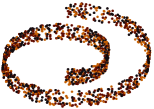
Maximum Variance Unfolding (MVU) [2] along with other manifold learning methods has addressed the problem of reducing the dimensionality of the data by preserving local distances. Most of the time the data end up living in a lower dimensional space. MVU explicitly finds the optimal kernel matrix for the data, by solving a semidefinite program. As a remark MVU usually gives the most compact spectrum [2], revealing the true intrinsic dimensionality of the dataset very well. The authors of the MVU point out though that it has very poor performance when it comes to using the kernel matrix for SVM classification [2] as it does not include any information about the linear separability of the classes. For example in figure 1b we show two classes on a Swiss roll manifold. After unfolding with MVU 1d, the classes remain non-linearly separable.
In this paper we introduce a variation of MVU that takes into consideration the linear separability of the classes. The result is a new algorithm, the Isometric Separation Mapping (ISM), that gives an unfolding that preserves the class structure of the manifold. The algorithm can be seen as a transductive (semi-supervised SVM), since it requires the test data during training. Previous work on transductive SVMs has also been studied by several researchers. When the choice of the kernel is ad-hoc, the problem becomes very difficult as it boils down to mixed integer programming [3]. In [4] and [5] the authors train the kernel matrix over a set of predefined kernels. Although this gives higher flexibility in forming the kernel, it might still require a large number of predefined kernels. For example if one of the choices was the Gaussian, it would be necessary to keep a large number of them with different sigmas (bandwidths). It is widely known that if the bandwidth of the Gaussian is too wide or too narrow kernel methods perform poorly. This technique usually leads to full rank Semidefinite programs that are computationally hard. Finally, in [6] the Laplacian Eigenmap framework is used for training SVMs. Laplacian Eigenmaps are another dimensionality reduction method based on the Gaussian kernel. It also tries to capture the local geometry and take advantage of it in SVM training. Our technique does not make any assumption on the kernel function. The only requirement is to preserve isometry on the data.
The paper is organized in the following way. In section 2 we give an overview of MVU along with its variants that make it scalable. In section 3 we present the ISM algorithm. Some examples on embedding manifolds with ISM are presented in 4. In section 5 we present a transductive SVM based on the ISM.
2 Maximum Variance Unfolding, Maximum Furthest Neighbor Unfolding.
Weinberger formulated the problem of isometric unfolding as a Semidefinite Programming algorithm [2].
Given a set of data , where is the number of points and is the dimensionality, the dot product or Gram matrix is defined as . The goal is to find a new Gram matrix such that in other words where and . Now the dataset is represented by which has fewer dimensions than . The requirement of isometric unfolding is that the euclidian distances in the for a given neighborhood around every point have to be the same as in the . This is expressed in:
where is the set of the indices of the neighbors of the point. From all the matrices MFNU chooses the one that maximizes the distances between furthest neighbor pairs and MVU the one that maximizes the variance of the set (equivalently the distances of the points from the origin). So the algorithm is presented as an SDP:
| (1) | |||||
| subject to | |||||
where the is the dot product between matrices. has the following form:
| (2) |
and
| (3) |
has the same structure of and computes the distance of the point with its furthest neighbor for MFNU, while for MVU it is just the unit matrix (computes the distance of the points from the origin). The last condition is just a centering constraint for the covariance matrix. The new lower dimensional representation of data is found in the eigenvectors of . In general MVU/MFNU gives Gram matrices that have compact spectrum, at least more compact than traditional linear Principal Component Analysis (PCA). The method behaves equally well with MVU. Unfortunately this method can handle datasets of no more than hundreds of points because of its complexity.
2.1 The Non Convex MVU/MFNU.
Kulis and Vasiloglou showed how the algorithm can be more scalable [7, 8] by replacing the constraint [9] with an explicit rank constraint . The problem becomes non-convex and it is reformulated to:
| subject to: | ||||
In [9], Burer proved that the above formulation has the same global minimum with the convex one. In this form the algorithm scales better.
3 Isometric Separation Maps (ISM)
Although MVU and its variant MFNU give low rank kernel matrices, experiments [2] show that they are performing poorly when it comes to SVM classification. In this section we will show that MVU/MFNU can be modified so that the kernel matrix can be used for classification too.
In traditional SVMs the kernel is chosen ad-hoc and the goal is to find a hyperplane that can linearly separate the classes. The kernel is chosen in such a way that it lifts the data in a high dimensional space hoping that data would be linearly separable. In our approach we have the hyperplane given and we are trying to find the kernel matrix that separates the data along the hyperplane. Finding a kernel matrix to satisfy that condition is trivial as it suffices to add one extra dimension on the data that will be either -1 or 1. What is sort of interesting though is to find a mapping to a (higher or lower) dimensional space that keeps data points linearly separable and preserves the local isometry. As we will see later, depending on the structure of the classes it is likely to end up in a higher dimensional space. We are interested in the minimum dimension of that space.
The solution of the problem is the following. We pick one of the data points to be normal to the separating hyperplane. The choice of the point does not matter since it will just change the orientation of the points in space. The manifold consists of two classes and . Let be the points that belong in the same class with , then , where is the generalized dot product between and . For points that belong to the opposite class , . Now the problem of MVU/MFNU with linear separability constraints can be cast as the following Semidefinite Program:
| (5) | |||||
| subject to | |||||
Using the same formulation as in [8] we can solve the above problem in a non-convex framework that scales better. Extending the problem for more classes is pretty straight forward. The only modification is to use more anchor points that will serve as normal vectors to the separating hyperplanes. The problem is always feasible provided that . 111As long as the k neighbors belong to the tangent space and the manifold is smooth, a folding (locally isometric transform) of the manifold along a hyperplane always exists [10]. If all pair distances are given then the Gram matrix is uniquely defined and the problem might be infeasible. In the trivial case where meaning that each point has exactly one neighbor then the problem is always feasible. In general there is a maximum k where the problem might become infeasible. That means there is always a where the training error is zero. That means we can always find a dimensional space where the Manifold can be embedded isometrically.
If some of the data points are labeled (training data) and some are not (test data), then the above method can be used as an SVM-like classifier that always achieves zero training error in contrast to other algorithms proposed for learning the kernel in SVM (mentioned in section 1 , where the kernel is learnt as a convex combination of preselected kernels). This might sound as over-fitting on the training data. In reality though this is not true since the test data participate during training glued on the training data with the distance constraints. Another remark on the ISM is that it is not a max margin classifier because it does not regularize the norm of the normal vector. It is not possible to do it since we need to also preserve the local distances.
4 Dimensionality Minimization with ISM
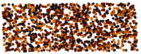
In order to verify ISM on dimensionality adjustment we tested it on the swiss roll dataset (1500 points). Two classes were defined on the swiss roll that were not linearly separable. ISM was performed on the dataset. Embedding in 2 dimensions was not possible as the isometry cannot be preserved (the algorithm terminated with 2% error on local distances). Embedding was though possible in 3 dimensions where the algorithm terminated with 0.01% error in the local distance constraints. In both cases the classification error was zero. As we see in fig. 1 MVU unfolds the dataset in a strip where the classes are not linearly separable.
a b
b
c d
d
e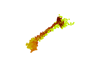 f
f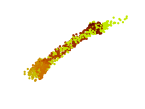
g h
h
The ISM on the other hand transforms the manifold in a set that preserves the local distances (k neighborhood=5) and divides the two classes in a linearly separable way. In order to demonstrate further the power of ISM we test it in two even more complex cases. In figure 2 we generated 3 classes on a swiss roll. Clearly MVU/MFNU unfolds the manifold in a non-separable way. ISM was able to map the swiss roll in a 12-dimensional space where the 3 classes are completely linearly separable.
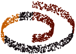
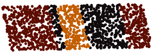
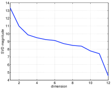
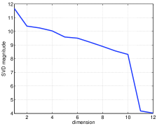
In figure 3 the Principal Component Analysis (PCA) spectrum of the 12 dimensional Swiss roll is shown. The spectrum is quite rich. ISM can handle even more complicated cases. In figure 3 we show 3 classes lying randomly on a Swiss roll. ISM was able to map the manifold in a 12-dimensional space keeping the 3 classes linearly separable. In figure 3 the PCA spectrum is depicted. The algorithm terminated with a very low feasibility error 0.4% for distance preservation and 0.16% for linear separability. Further improvement of the feasibility error was possible, but L-BFGS becomes slow as it goes close to the optimum. In general the algorithm converges very quickly to 1% feasibility error. Further improvement is possible but takes time.
5 Transductive SVMs
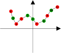
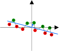
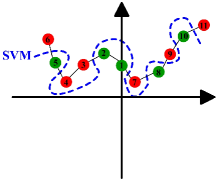
The method described above can also be used as a transductive SVM in a semi-supervised setting. Transductive SVMs are in general difficult problems. If the kernel is preselected then a mixed integer problem has to be solved. If the kernel is learnt from the data then as we mentioned earlier no guarantee can be given that the training data are linearly separable. In ISM the kernel is trained over all data, using all neighborhood information. After solving the optimization problem, the classification information for the test data will be on the sign of , where is the test set. At this point we would like to highlight the difference between SVMs and ISMs. In figure 5 we see how SVMs and ISMs would classify points. SVMs keep the points fixed and try to find the optimal curve that separates the points. ISMs picks the hyperplane and moves the points around it (always keeping them connected), so that they are correctly classified.
In order to evaluate ISM as an SVM classifier we chose a publicly available dataset and compared them versus traditional SVMs in two different modes. We used the publicly available SVM-light software for traditional SVM classification. In the first experiment we picked 1000 points from the magic gamma telescope dataset, publicly available at the UCI repository. We chose 50 points as training points and used the other 950 as test points. For traditional SVM classification we tested the linear, Gaussian and polynomial kernel, with different parameters for the the bandwidth and the polynomial order. We also tuned the regularization factor so that the test error was minimized. In other words we pushed traditional SVMs to their best performance. The critical parameter for ISM SVM is the k-neighborhood. Usually small values of k allow embedding in lower dimensional spaces, while large k lead in higher dimensional ones. In tables 1,2 the results are summarized. We tested several k-neighborhoods for ISM and different Kernels for traditional SVMs. From the results we observe that ISM behaves slightly better that SVM (73.68% versus 70.32%). This is mainly because the training set is small and SVM cannot capture very well the geometry.
In the second experiment we use the whole dataset. The training set contains 12080 datapoints and the test set 6340. Although the dataset is 10 dimensional, it is possible to reduce its dimension with MVU/MFNU down to 5. In order to make it linearly separable though with ISM it was necessary to use more than 10. In tables 3, 4 the results are summarized. As we can see SVM performs slightly better than ISM (83.28% versus 81.00%). Another remark in both cases is that ISM always behaves better than the linear kernel. Gaussian SVM performance has the best performance. This is expected since Gaussian matrices are usually full rank. ISM uses kernel matrices of much smaller rank and they achieve equivalent performance.
The results don’t necessarily demonstrate big difference between SVMs and ISM. We also experimented with some toy datasets, such as the half moon dataset presented in [6]and a Swiss roll, where one data point is given per class. ISM obviously behaves better than SVM but this is a trivial and not a fair comparison. In general the differences between ISM and traditional SVMs are in the same levels with the results reported in other transductive SVM papers [6, 4].In practice ISMs are slower than SVMs since they are Semidefinite Problems contrary to SVMs that solve Quadratic problems. It is interesting though that they provide an tool for associating the dimensionality of the dataset with the classification score and linear separability. The more we increase the dimensionality of the dataset with ISM the better the classification score. In fact k acts as a regularizer. Large values of k correspond to better generalization of the SVM as the test error drops.
| k-NEIGHBORS | DIMENSION | SCORE |
|---|---|---|
| 5 | 50 | 70.10% |
| 8 | 10 | 68.73% |
| 10 | 12 | 70.63% |
| 15 | 8 | 70.42% |
| 15 | 12 | 69.05% |
| 20 | 8 | 71.68% |
| 20 | 12 | 71.68% |
| 20 | 40 | 73.37 |
| 25 | 8 | 72.63% |
| 25 | 12 | 71.89% |
| 30 | 40 | 73.68% |
| KERNEL | PARAMETER | SCORE |
|---|---|---|
| Gaussian | 0.1 | 69.89% |
| Gaussian | 0.5 | 70.00% |
| Gaussian | 1.0 | 70.11% |
| Gaussian | 1.5 | 70.00% |
| Gaussian | 2.0 | 70.11% |
| Gaussian | 4.0 | 70.21% |
| Gaussian | 5.0 | 70.32% |
| Gaussian | 6.0 | 70.21% |
| Gaussian | 8.0 | 70.11% |
| linear | - | 69.89% |
| polynomial | 1 | 69.89% |
| polynomial | 2 | 69.68% |
| polynomial | 3 | 69.58% |
| polynomial | 4 | 69.84% |
| polynomial | 5 | 68.84% |
| polynomial | 6 | 68.84% |
| polynomial | 8 | 68.95% |
| k-NEIGHBORS | DIMENSION | SCORE |
|---|---|---|
| 12 | 30 | 80.22% |
| 12 | 35 | 79.97% |
| 12 | 40 | 80.47% |
| 12 | 45 | 79.76% |
| 12 | 50 | 79.81% |
| 12 | 55 | 81.00% |
| 15 | 40 | 80.39% |
| 15 | 45 | 79.40% |
| 15 | 50 | 79.07% |
| 15 | 55 | 79.82% |
| 20 | 40 | 78.96% |
| 20 | 45 | 79.68% |
| 20 | 50 | 80.13% |
| 20 | 55 | 78.42% |
| k-NEIGHBORS | DIMENSION | SCORE |
|---|---|---|
| Gaussian | 8 | 83.28% |
| Gaussian | 6 | 82.77% |
| linear | - | 78.64% |
| polynomial | 2 | 81.62% |
| polynomial | 3 | 82.07% |
| polynomial | 5 | 81.26% |
6 Summary
In this paper we presented a new Manifold Learning method the Isometric Separation Maps. This method is ideal for reducing the dimension of Manifold with class information associated with them. We also showed how ISM can be used as semi-supervised (transductive) classifiers. Although they don’t have superior performance compared to traditional max margin SVMs, they are a useful tool for determining the dimensionality of the kernel space that is necessary for achieving linear separability. We believe that some improvement of the objective function is necessary so that generalization is improved. Probably a term minimizing the norm of the vector normal to the hyperplane (as in SVMs) can be used.
References
- [1] J. Shawe-Taylor and N. Cristianini, Kernel Methods for Pattern Analysis, Cambridge University Press New York, NY, USA, 2004.
- [2] K.Q. Weinberger, F. Sha, and L.K. Saul, “Learning a kernel matrix for nonlinear dimensionality reduction,” in ICML. ACM New York, NY, USA, 2004.
- [3] K. Bennett and A. Demiriz, “Semi-Supervised Support Vector Machines,” NIPS, 1999.
- [4] G.R.G. Lanckriet, N. Cristianini, P. Bartlett, L. El Ghaoui, and M.I. Jordan, “Learning the Kernel Matrix with Semidefinite Programming,” JMLR, vol. 5, pp. 27–72, 2004.
- [5] S.J.Z. Kim, A. Magnani, A.K. Koh, and S. Boyd, “Learning the kernel via convex optimization,” in ICASSP, 2008, pp. 1997–2000.
- [6] M. Belkin, P. Niyogi, and V. Sindhwani, “On manifold regularization,” in AISTAT, 2005.
- [7] B. Kulis, A.C. Surendran, and J.C. Platt, “Fast Low-Rank Semidefinite Programming for Embedding and Clustering,” in AISTATS, 2007.
- [8] N. Vasiloglou, A. Gray, and D. Anderson, “Scalable Semidefnite Manifold Learning,” in MLSP, 2008.
- [9] S. Burer and R.D.C. Monteiro, “A nonlinear programming algorithm for solving semidefinite programs via low-rank factorization,” Mathematical Programming, vol. 95, no. 2, 2003.
- [10] J.M. Lee, Introduction to Smooth Manifolds, Springer, 2003.