myctr
Specification of a Microscopic Pedestrian Model by Evolutionary Adjustment to Video Tracking Data
Abstract
Based on suitable video recordings of interactive pedestrian motion and improved tracking software, we apply an evolutionary optimization algorithm to determine optimal parameter specifications for the social force model. The calibrated model is then used for large-scale pedestrian simulations of evacuation scenarios, pilgrimage, and urban environments.
keywords:
Evolutionary optimization; pedestrian interaction; video tracking; social force model; pedestrian simulation; evacuation scenarios1 Introduction
In recent years, pedestrian research has become a very active field. Queueing-theoretical approaches (see, e.g., Refs. [25, 23]) and fluid-dynamic models [6, 16, 17] have facilitated insights into the large-scale dynamics of pedestrian crowds, in particular into the phenomon of intermittent flows and stop-and-go traffic emerging at extreme densities [11]. However, most recent work is dedicated to microscopic simulation models such as the social force model [8, 9, 10, 14, 38], cellular automata [20, 21, 30], particle hopping models [27], and others, e.g. multi-agent approaches [37, 1].
While some of these models are aiming at the simulation of real evacuation scenarios, others are focussing on an understanding of the self-organized dynamical patterns that a realistic model must also be able to reproduce. But how to calibrate these models? One common method is to modify model parameters and model components long enough until the simulations fit the fundamental flow-density diagram such as the one proposed by Weidmann [35]:
| (1) |
This method can certainly be applied, but it does not necessarily lead to realistic and reliable simulation results. First of all, the fundamental diagram depends enormously on the body size distribution [31] and other characteristic features of the crowd Second, most models fitting the fundamental diagram must be separately calibrated to many differen situations, as they do not reproduce the various dynamical phenomena in pedestrian crowds well. These phenomena include the formation of lanes of uniform walking direction in crowds with oppositely moving pedestrians, stripe formation in two intersecting pedestrian streams, and oscillations of the passing direction at bottlenecks under normal conditions with moderate densities [12, 9].
Apart from the latter two phenomena, which have been discovered only recently, the social force model, despite its simplicity, has been shown to reproduce the dynamics in crowds qualitatively well. However, not much effort has been spent in the past to calibrate it for the application to dimensioning and evacuation problems. We will, therefore, introduce a method to calibrate microscopic pedestrian simulation models using trajectory data reflecting pedestrian interactions, and apply it to the social force model.
Our paper is organized as follows: Section 2 will shortly introduce the social force model and some specifications of it. In Sec. 3, we will then introduce our method to optimize parameters based on trajectory data. For this, we will shortly describe the video tracking method applied to gain the trajectory data. Moreover, we will discuss how the data can be used to determine the interaction forces themselves. Afterwards, in Section 4 we will present some examples of large-scale pedestrian and evacuation simulations. Finally, Sec. 5 will summarize and conclude our paper.
2 Specifications of the Social Force Model
The social force model can be underpinned with a social science model of behavioral changes proposed by Lewin [22]. He has introduced the idea that behavioral changes were guided by so-called social fields or social forces. This idea has been put into mathematical form by Helbing [4] and applied to opinion formation [7], pedestrian motion [5], and vehicle traffic [33]. The social force model for pedestrians assumes that each individual is trying to move in a desired direction with a desired speed , and that it adapts the actual velocity to the desired one, within a certain relaxation time . The velocity , i.e. the temporal change of the location , is itself assumed to change according to the acceleration equation
| (2) |
where is a fluctuation term and the systematic part of the acceleration force of pedestrian given by
| (3) |
The terms , denote the repulsive forces describing the attempts to keep a certain safety distance to other pedestrians and obstacles . The fluctuation term reflects random behavioral variations arising from deliberate or accidental deviations from the average way of motion. The above equation are nonlinearly coupled Langevin equations and can be solved numerically using Euler’s method. In very crowded situations, additional physical contact forces come into play [10].
For the time being, we will assume a simplified interaction force of the form
| (4) |
where is the distance vector pointing from pedestrian to and the angle between the normalized distance vector and the direction of motion of pedestrian , i.e. . It has, for example, been suggested to reflect by the function
| (5) |
that the reaction of pedestrians to what happens in front of them is much stronger than to what happens behind them. Here, with is a parameter which grows with the strength of interactions from behind. Later on, we will try to determine this angular dependence from video tracking data. The distance dependence has been specified in different ways. We will start with the circular specification of the interaction force,
| (6) |
where and denote something like the radii of pedestrians and , while and are parameters. reflects the strength of interaction, while corresponds to the interaction range. While the dependence on explicitly allows for a dependence of these parameters on the single individual, we will assume and in the following. Otherwise, it would be hard to collect enough data for parameter calibration.
3 Evolutionary Model Specification Via Video Tracking
Let us now turn to the question how the parameters and and the angular interaction strength can be determined from video recordings.
3.1 Video Tracking Method
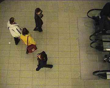
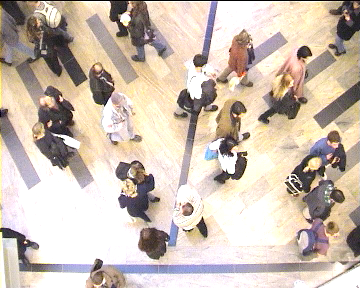
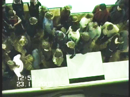
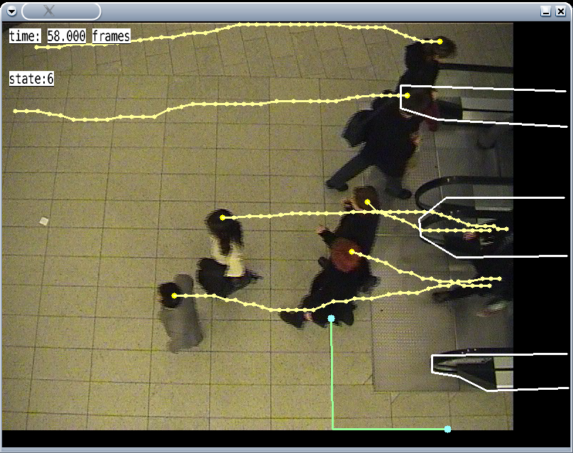
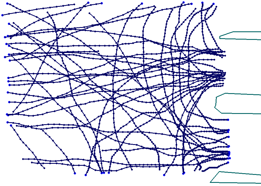
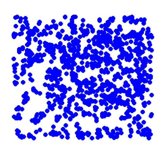
We have made several video recordings of pedestrian crowds in different natural environments in Budapest (Hungary) and Stuttgart (Germany) from the top (see Fig. 1). The dimensions of the recorded areas was known, and the floor tiling or environment provided something like a “coordinate system”. The heads were automatically determined by seaching for round moving structures, and the accuracy of tracking was improved by comparing actual with linearly extrapolated positions (so it would not happen so easily that the algorithm interchanged or “lost” closeby pedestrians). The trajectories of the heads were then projected on two-dimensional space in a way correcting for distortion by the camera perspective. A representative plot of the resulting trajectories is shown in Fig. 2. However, it should be noted that extracting trajectory data from pedestrians is nothing new. It has been done in the past with infra-red sensors [19] or video recordings [15, 31].
3.2 Parameter Optimization by an Evolutionary Algorithm
For model calibration, we have used a hybrid method fusing empirical trajectory data and microscopic simulation data of pedestrian movement in space. To each tracked pedestrian, we have assigned a virtual pedestrian in the simulation domain. We have then started a simulation for seconds, in which one pedestrian was moved according to a simulation of the social force model, while the others were moved exactly according to the trajectories extracted from the videos. This procedure was performed for all pedestrians and for several different starting times , using a fixed parameter set for the social force model.
Each simulation run was performed according to the following scheme:
-
1.
Define a starting point and calculate the state (position , velocity , and acceleration ) for each pedestrian .
-
2.
Assign a desired speed to each pedestrian. In our simulations, we have specified it by the maximum speed during the pedestrian’s tracking time, which is sufficiently accurate if the overall pedestrian density is not too high and the desired speed is constant in time.
-
3.
Assign a desired goal point for each pedestrian. We have assumed is would correspond to the point at the end of the trajectory.
-
4.
Given the tracked motion of the surrounding pedestrians , simulate the trajectory of pedestrian based on the social force model during seconds of time, starting at the actual location .
After each run, we determined the relative distance error
| (7) |
After averaging the relative distance errors over the pedestrians and starting times , the negative value of the result was taken as fitness of the parameter set used in the pedestrian simulation.111Note that we have actually averaged over the 30% central values of the relative distance errors only in order to remove outliers due to untypical, unreasonable, or exceptional pedestrian behaviors. Hence, the best possible value of the fitness was 0, but any deviation from the real pedestrian trajectories would imply negative fitness values.
Moreover, with the fitness measure outlined above, we have used a simple evolutionary algorithm to obtain the parameter set with the highest fitness value, which was . This value reflects in some sense the stochasticity and/or heterogeneity of individual behaviors. For comparison, we also made simulations with , i.e. without any social forces, assuming that persons will never change their velocity. This measurement resulted in a fitness value of .
3.3 Improved Specifications of the Social Force Model
3.3.1 Velocity-Dependent Interaction Forces
Interactions among pedestrians are actually more complicated than suggested above. For example, it is know that the angle matters, at which two pedestrians and approach each other (which is given by ). Apart from this, the step sizes and, therefore, the speeds matter as well. In the following, we will shortly discuss two anisotropic models of pedestrian interactions:
Elliptical specification I: In Ref. [13], a generalization of Eq. (6) was formulated, which assumed that the repulsive potential
| (8) |
is an exponentially decreasing function of with equipotential lines having the form of an ellipse directed into the direction of motion as shown in Fig. 3. The semi-minor axis was determined by
| (9) |
in order to take into account the length of the stride (step size) of pedestrian , where . The reason for this specification was that pedestrians require space for movement, which is taken into account by other pedestrians.
The repulsive force is related to the repulsive potential via
| (10) |
Considering the chain rule, , and , this leads to the explicit formula
| (11) |
with . For , we regain the expression of Eq. (6).

Elliptical specification II: Recently, a variant of this approach has been proposed [32], assuming
| (12) |
The special feature of this approach is its symmetrical treatment of both pedestrians and .
In order to compare the elliptical specifications with the circular one, let us make the following thought experiments:
-
•
Scenario 1: Consider a pedestrian walking towards a wall with a given speed , but four different orientations (with ), as shown in Fig. 4. This scenario can be treated analogously to the movement relative to a standing pedestrian , which implies .
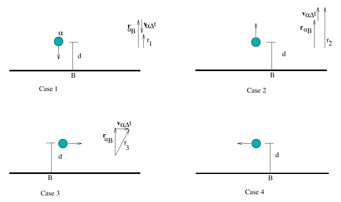
Figure 4: Illustration of scenario 1, in which pedestrians are walking at a given speed in different directions close to a wall. Then, in case II the repulsive force is a monotonously decreasing function of given by
(13) according to Eq. (12). For all four cases, the values of and (the step size of pedestrian ) are the same, but the values of are different. We have , so that we find for the magnitudes of the repulsive forces triggered by the wall (as the direction of the forces is perpendicular to the wall in all four cases.) This agrees well with experience, i.e. the anisotropic and orientation behavior of pedestrians are realistically reproduced by the elliptical force specification II. In contrast, the elliptical model I implies according to Eq. (9) and predicts the same force in all four cases, as does the circular model.
-
•
Scenario 2: Consider single pedestrians walking towards a wall, but with 2 different velocities as shown in Fig. 5. Obviously, the elliptical specification II predicts that the pedestrian with the higher speed would decelerate earlier, as expected. In contrast, the elliptical model I and the circular interaction model are insensitive to the own speed .

Figure 5: Illustration of scenario 2, in which pedestrians are walking with different speeds towards a wall. -
•
Scenario 3: Consider the case of two pedestrians walking towards each other with different velocities , as shown in Fig. 6.

Figure 6: Illustration of scenario 3, in which pedestrian are walking towards each other with different velocities. While the circular interaction force does not imply any velocity-dependence of pedestrian behavior, the elliptical formulations do, which is certainly more realistic. The first elliptical model assumes a velocity-dependence of pedestrian interactions, but no sensitivity with respect to the own speed. Therefore, specification II is expected to be more realistic.
For the above reasons, we will not consider the elliptical specification I anymore, but focus on the elliptical model II.
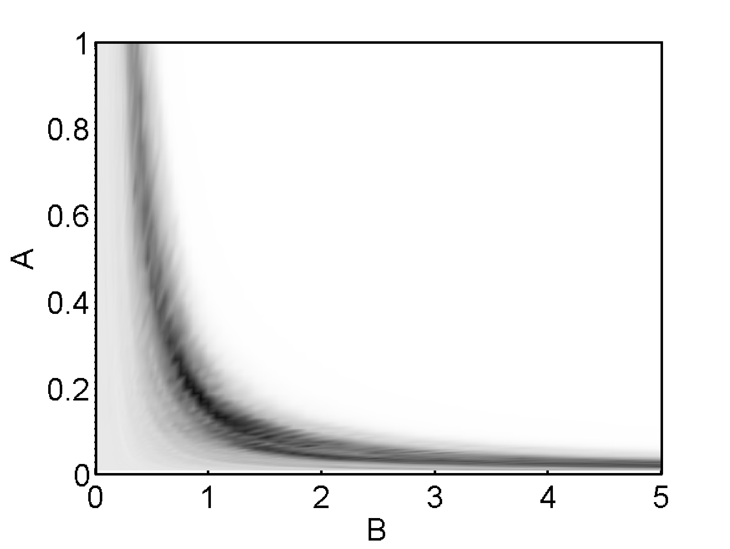
Figure 7 represents the resulting fitness values as a function of the choice of the interaction strength and the interaction range , assuming .
| Model | A | B | Fitness | |
|---|---|---|---|---|
| Extrapolation | 0 | – | – | -0.66 |
| Circular | 0.42 0.26 | 1.65 1.01 | 0.12 0.07 | -0.60 |
| Elliptical I | 0.11 0.01 | 1.19 0.45 | 0.16 0.04 | -0.59 |
| Elliptical II | 0.04 0.01 | 3.22 0.67 | 0.06 0.04 | -0.39 |
| Circular | 0.11 0.06 | 0.84 0.63 | 1 | -0.65 |
| Elliptical I | 1.52 1.65 | 0.21 0.08 | 1 | -0.67 |
| Elliptical II | 4.30 3.91 | 1.07 1.35 | 1 | -0.47 |
One result of our parameter optimization was that, for each video, there was actually a broad range of parameter combinations of and which performed almost equally well, while the optimal value of the anisotropy parameter was . This allowed us to apply additional goal functions in our optimization. We used this fact to determine among the best performing parameter values such parameter combinations, which performed well for all three video recordings, using a fitness function which weighted the fitness reach in each single video equally (i.e. with a factor 1/3).
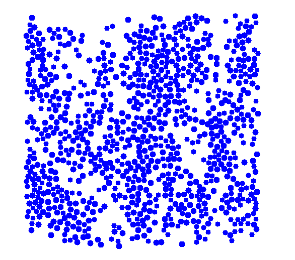
The resulting parameters are listed in Table 1. The parameters corresponding to the best fitness value, i.e. the elliptical specification II with , were used in a microscopic simulation with periodic foundary conditions, and the resulting fundamental diagram, is shown in Fig. 8. The solid line is the Weidmann curve, Eq. (1), Note that, with additional fine tuning, it will be possible to make an even better fit to the Weidmann fundamental diagram, but here we rather just show that extracting parameters from videos and perform a microscopic simulation will correspond to dynamics close to the empirical flow-density relation.

We would, however, like to mention that further velocity-dependent specifications of pedestrian interaction forces were proposed in the past, for example, by Molnár Ref. [26, 8], Okazaki [28], Hoogendoorn [14], and Yu [38].
Although, from a theoretical perspective, velocity-dependent force specifications are more promising than the circular interaction force introduced in the beginning, it turns out that the prediction of pedestrian motion does not become a lot better by including additional, speed-dependent parameters. This is illustrated by the fitness values in Table 1. Obviously, the deviation of the fitness value from 0 is mainly caused by the heterogeneity of pedestrian behaviors. A similar conclusion has been drawn from studies specifying behavioral parameters in different car-following models [3].
3.3.2 Angular Dependence of Pedestrian Interactions
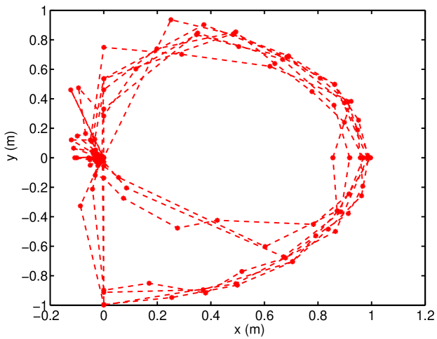
Our evolutionary fitting method can be also used to determine interaction laws without prespecified interaction functions. For example, one can determine the angular dependence of pedestrian interaction directly. In order to do this, we have chosen an approach using a polygon with edges in the directions . The distance of the curve in direction from the origin represents the (relative) angular interaction strength with a maximum value of 1. To get some smoothness, linear interpolation has been applied between each of the edges. Figure 10 shows the angular dependence of the interaction strength determined from pedestrian trajectories. Apparently, pedestrians are only sensitive to what happens inside an degree angle in front of him or her, which roughly corresponds to the visually perceived area.
3.3.3 Distance Dependence of Pedestrian Interactions
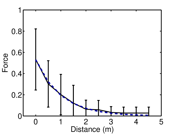
In a similar way, we have determined the distance dependence of pedestrian interactions without a pre-specified function. For this, we have adjusted the values of the force at given distances (with ) in an evolutionary way. The resulting fit curve is presented in Fig. 11. According to our results, the empirical dependence of the force with distance can be well fitted by an exponential decay, as assumed before. Note that similar studies have been carried out for vehicle interactions, recently [34]. However, the situation for pedestrians is more difficult due to their two-dimensional motion. Therefore, our evolutionary fitting procedure seems to be superior to the Fokker-Planck approach (or Random Matrix Theory approach), which was used to calibrate vehicle interactions.
4 Large-Scale Pedestrian and Evacuation Simulations
In the following section, we will present some examples for large-scale pedestrian simulations with the social force model. For simplicity and computational speed, we have assumed circular pedestrian interactions, here. Compared to previous implementations of the model, numerical efficiency has been increased a lot, for example by cutting off interation forces at a certain, large enough distance (around m) and book-keeping of neighboring pedestrians. In this way, the simulation of 30,000 pedestrians or more in real-time is no problem. Larger crowds have been simulated off-line or using parallel computing.
For example, a simulation have been performed for an evacuation of two decks of a ship connected by a staircase. The underlying study has shown that the model is also suitable for treating different personalities (the different characteristic behaviors in emergency situations), complex geometries, and three-dimensional interactions [36]. A simulation [14] have been performed for multi-destination flows at Schiphol airport in the Netherlands, while [24] have simulated the evacuation of an exhibition area, both with the social force model. For a similar simulation see Fig. 12.
Our model has also been used to simulate pedestrian flows on the Jamarat Bridge, which has to cope with 3 million pilgrims within a single day (AlGadhi and Mahmassani, 1990). Figure 13 illustrates the scenario for the old Jamarat bridge. It shows the development of zones of high density and pressure behind the previous circular basins. In the middle of each of the three basins is a pillar symbolizing the devil. These pillars are to be stoned with seven pebbles each, which takes time and delays pedestrian motion. This, in turn, can cause extreme crowding. Note, however, that the situation around the pillars has significantly improved since the circular stoning areas were replaced by elliptical ones.


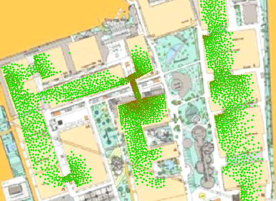
As indicated before, the implementation of our pedestrian microsimulator has been optimized for efficiency and scalability in terms of computational speed and memory. It is no problem to simulate more than 30,000 pedestrians in real-time on a normal PC. Parallel computing even allows one to simulate more than 100,000 pedestrians in real-time. This is suitable for the simulation of large scenarios such as pedestrian flows in extended urban areas (see Fig. 14) or during mass events such as street parades or carnivals [1].
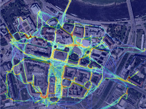
In order to be suitable for scenarios of this complexity, we have developed a powerful and flexible pedestrian simulator called “UNIVERSE”, in which we have implemented certain additional features complementing the social force model:
-
1.
a powerful scenario generation module based on XML,
-
2.
path finding and route choice modules to describe the selection of destinations, including spontaneous stops and impluse shopping,
-
3.
calibration modules to adapt simulations to real measurements,
-
4.
a statistics module evaluating various performance measures (such as densities, velocities, flow efficiency, pressure, overall evacuation time, etc.) to assess and compare different scenarios,
-
5.
an optimization module based on evolutionary algorithms which allows to improve the geometrical boundary conditions of pedestrian facilities,
-
6.
various visualization modes for the illustration of the simulation results, both on- and off-line, and
-
7.
a functionality reflecting density-dependent herding effects.
5 Summary and Outlook
Tracking algorithms have become a powerful tool for empirical data evaluation, recently [15, 31, 19]. In our study, we have further developed and applied this tool to determine trajectories of many interacting pedestrians. These trajectories were used to calibrate a microscopic pedestrian model, namely the social force model. For this, we have simulated single pedestrians, given the measured motion of the other pedestrians. The difference between simulated and measured pedestrian behavior has then been minimized through evolutionary variation of the model parameters. However, it was also possible to determine the distance- and angle-dependencies of the interactions directly. In this way, the previously assumed exponentially decay of the interaction strength with distance was empirically confirmed.
It turned out that the simplest specification of the interaction forces in the social force model almost performed as well as velocity-dependent specifications with more parameters. We have, therefore, used the circular specification for our large-scale simulations, which is in favor of computational speed. With some simplifications for the sake of numerical performance, it is no problem to simulate scenarios with 30,000 pedestrians on-line on a normal PC. Larger crowds can be simulated off-line or using parallel computing. This allows one to study pedestrian zones, convention halls, shopping malls, airports, railway stations, city festivals, etc. There are, by the way, also special algorithms for the evolutionary optimization of highly frequented areas [18]. Hence, pedestrian simulations are now a useful tool for the planning of pedestrian facilities and mass events, if properly calibrated.
Note, however, that that measurement and calibration results should be transfered from one place to another only with care, as the maximum flow and density values are largely influenced by the body size distribution. Other factors may play a role as well, for example the age distribution, the fraction of handicapped people, the carrying of luggage, alcohol consumption, cultural habits, use of mobile phones, and the situational context [29] (e.g. business, leisure, sports, or religious activities). All of this should be taken into account in the dimensioning of pedestrian facilities, safety (evacuation) analyses, and the calibration of computer models.
Acknowledgements
The authors would like to thank Peter Felten for his work with the video material and the German Research Foundation (DFG project He 2789/7-1) for financial support. Further on, the authors are thankful to Serge Hoogendoorn for providing empirical data, used to verify the results, shown in figures 10 and 11.
References
- [1] Batty, M., Desyllas, J., and Duxbury, E., The discrete dynamics of small-scale spatial events: agent-based models of mobility in carnivals and street parades, Int. J. Geographical Information Science 17(7), 673-697 (2003).
- [2] Daamen, W., and Hoogendoorn, S. P., Experimental research of pedestrian walking behaviour, Transportation Research Records 1828, 20-30 (2003).
- [3] Eissfeldt, N. and Wagner, P., Effects of anticipatory driving in a traffic flow model, The European Physical Journal B - Condensed Matter 33(1), 121-129 (2003).
- [4] Helbing, D., A mathematical model for the behavior of pedestrians, Behavioral Science 36, 298-310 (1991).
- [5] Helbing, D., A mathematical model for the behavior of pedestrians, Behavioral Science 36, 298-310 (1991).
- [6] Helbing D., A fluid-dynamic model for the movement of pedestrians, Complex Systems 6, 391-415 (1992).
- [7] Helbing, D., A mathematical model for the behavior of individuals in a social field, Journal of Mathematical Sociology 19 (3), 189-219 (1994).
- [8] Helbing, D., Verkehrsdynamik. Neue physikalische Modellierungskonzepte (Springer, Berlin, 1997).
- [9] Helbing, D., Buzna, L., Johansson, A., and Werner, T., Self-organized pedestrian crowd dynamics: Experiments, simulations, and design solutions, Transportation Science 39, 1-24 (2005).
- [10] Helbing, D., Farkas, I., and Vicsek, T., Simulating dynamical features of escape panic, Nature 407, 487-490 (2000).
- [11] Helbing, D., Johansson, A., Mathiesen, J., Jensen, M. H., and Hansen, A., Analytical Approach to Continuous and Intermittent Bottleneck Flows, submitted (2006).
- [12] Helbing, D., Molnár, P., Farkas, I., and Bolay, K., Self-organizing pedestrian movement, Environment and Planning B 28 361-383 (2001).
- [13] Helbing, D. and Molnár, P., Social force model for pedestrian dynamics, Physical Review E 51, 4282-4286 (1995).
- [14] Hoogendoorn, S.P., Walker Behaviour Modelling by Differential Games, in Proceedings of the Computational Physics of Transport and Interface Dynamics Seminar, (Springer, 2002).
- [15] Hoogendoorn, S. P., Daamen, W., Bovy, P. H. L., Extracting microscopic pedestrian characteristics from video data, Annual Meeting Transportation Res. Board Pre-print CD-Rom, Mira Digital Publishing, Washington, D.C (2003).
- [16] Hughes, R.L., A Continuum Theory of Pedestrian Motion, Transportation Res. B, 507-535 (2002).
- [17] Hughes, R.L., The Flow of Human Crowds, Annual Rev. Fluid Mech., 169-182 (2003).
- [18] Johansson, A. and Helbing, D., Pedestrian Flow Optimization with a Genetic Algorithm Based on Boolean Grids, in Pedestrian and Evacuation Dynamics ’05, (Springer, Berlin, 2005), in print.
- [19] Kerridge, J. and Chamberlain, T., Collecting Pedestrian Trajectory Data In Real-time, in Pedestrian and Evacuation Dynamics ’05, (Springer, Berlin, 2005), in print.
- [20] Kirchner, A., Klüpfel, H., Nishinari, K., Schadschneider, A., and Schreckenberg M., Discretization effects and the influence of walking speed in cellular automata models for pedestrian dynamics, J. Stat. Mech.: Theor. Exp. P10011 (2004).
- [21] Klüpfel, H., Meyer-König, T., and Schreckenberg, M., Microscopic modelling of pedestrian motion—Comparison of an evacuation exercise in a primary school to simulation results, in Traffic and Granular Flow ’01, eds. Fukui, M. et al., (Springer, Berlin, 2003).
- [22] Lewin, K., Field Theory in Social Science, Harper & Brothers, New York, (1951).
- [23] Løvås, G. G. in Modelling and Simulation 1993, (Lyon, France, 1993) pp. 469–473.
- [24] Marinova, R., Ourdev I., and Stoilov V., Pedestrian motion in realistic virtual reality environments: application to high-rise building evacuation, in Pedestrian and Evacuation Dynamics 2003, eds. Galea, E. R., (CMS Press, London, 2003), pp. 283-293.
- [25] Mayne, A. J., Biometrica 41, 375–389 (1954).
- [26] Molnár, P., Modellierung und Simulation der Dynamik von Fußgängerströmen, PhD Thesis, Shaker (1996).
- [27] Muramatsu, M., Irie, T., and Nagatani, T., Jamming transition in pedestrian counter flow, Physica A 267 487 (1999).
- [28] Okazaki, S., A Study of Pedestrian Movement in Architectural Space, Part 1: Pedestrian Movement by the Application on of Magnetic Models, Trans. of A.I.J. (1979).
- [29] Predtetschenski, W. M. and Milinski, A. I., Personenströme in Gebäuden – Berechnungsmethoden für die Projektierung –, Rudolf Müller, Köln-Braunsfeld, (1971).
- [30] Schadschneider, A., Cellular Automaton Approach to Pedestrian Dynamics - Theory, in Pedestrian and Evacuation Dynamics, eds. Schreckenberg, M. and Sharma, S.D., (Springer, 2001), pp. 75.
- [31] Teknomo, K., Microscopic Pedestrian Flow Characteristics: Development of an Image Processing Data Collection and Simulation Model, PhD Thesis, Japan (2002).
- [32] Shukla, P. K. Modeling and Simulation of Pedestrians, Diploma Thesis (2005).
- [33] Tilch, B. and Helbing, D. Evaluation of single vehicle data in dependence of the vehicle-type, lane, and site, in Traffic and Granular Flow ’99: Social, Traffic, and Granular Dynamics, eds. D. Helbing, et al., (Springer, Berlin, 2000), pp. 333-338.
- [34] Treiber, M., Kesting, A., and Helbing, D., Delays, inaccuracies and anticipation in microscopic traffic models, Physica A 360, 71-88 (2006).
- [35] Weidmann, U., Transporttechnik der Fußgänger. ETH-Zürich, Schriftenreihe IVT-Berichte 90, Zürich (1993).
- [36] Werner, T. and Helbing, D., The social force pedestrian model applied to real life scenarios, in Pedestrian and Evacuation Dynamics 2003, eds. Galea, E. R., (CMS Press, London, 2003), pp. 17-26.
- [37] Willis, A.,, Kukla, R., Hine, J., and Kerridge, J., Developing the behavioural rules for an agent-based model of pedestrian movement, presented at the 25th European Transport Congress, Cambridge, UK (2000).
- [38] Yu, W. J., Chen, R., Dong, L. Y., and Dai, S. Q., Centrifugal force model for pedestrian dynamics, Phys. Rev. E 72, 026112 (2005).