Interplay between interaction and (un)correlated disorder in one-dimensional many-particle systems: delocalization and global entanglement

Abstract

We consider a one-dimensional quantum many-body system and investigate how the interplay between interaction and on-site disorder affects spatial localization and quantum correlations. The hopping amplitude is kept constant. To measure localization, we use the number of principal components (NPC), which quantifies the spreading of the system eigenstates over vectors of a given basis set. Quantum correlations are determined by a global entanglement measure $Q$, which quantifies the degree of entanglement of multipartite pure states. Our studies apply analogously to a one-dimensional system of interacting spinless fermions, hard-core bosons, or yet to an XXZ Heisenberg spin-1/2 chain. Disorder is characterized by both: uncorrelated and long-range correlated random on-site energies. Dilute and half-filled chains are analyzed. In half-filled clean chains, delocalization is maximum when the particles do not interact, whereas multi-partite entanglement is largest when they do. In the presence of uncorrelated disorder, NPC and Q show a non-trivial behavior with interaction, peaking in the chaotic region. The inclusion of correlated disorder may further extend two-particle states, but the effect decreases with the number of particles and strength of their interactions. In half-filled chains with large interaction, correlated disorder may even enhance localization.

I Introduction

Disorder may significantly affect the properties of physical systems. Spatial localization of one-particle states (Anderson localization), for example, is due to uncorrelated random disorder Anderson (1958); Lee and Ramakhrishnan (1985); Lifshitz et al. (1998); Kramer and MacKinnon (1993); whereas short range Flores (1989); Dunlap et al. (1990); Sánchez et al. (1993) and long range correlated de Moura and Lyra (1998); Izrailev and Krokhin (1999) disorder have been associated with the appearance of delocalized states. Interestingly, however, a recent experiment Kuhl et al. (2008) shows that long-range correlated disorder may in fact either suppress or enhance localization. This scenario becomes yet more complex when two or more particles are considered and the effects of interactions are taken into account. A clear picture of the interplay between interaction and disorder is essential to advance our understanding of thermodynamic and kinetic properties, as well as the dynamical behavior of real quantum many-body systems.

The interest in how interactions influence localization and transport properties of mesoscopic systems was boosted with the realization that persistent currents could only be explained if the role of the electron-electron interaction was addressed Guhr et al. (1998). In general, interaction between particles in disordered systems may lead to delocalization Chui and Bray (1977); Apel and Rice (1982); Kagan1984 ; Giamarchi and Schulz (1988); Dorokhov (1990); Shepelyansky (1994); Evangelou et al. (1996); Abrahams et al. (2001); Nascimento et al. (2005); Dias et al. (2007). The competition between interaction and disorder in many-body systems relates also to other interesting phenomena, such as the rich variety of quantum phase transitions of ultracold atomic Bose gases in optical lattices Roth and Burnett (2003), the transition from integrability to chaos Georgeot and Shepelyansky (1998); Avishai et al. (2002); Santos (2004) in spin systems, and the enhancement of entanglement Santos et al. (2004); Lakshminarayan and Subrahmanyam (2005); Mejia-Monasterio et al. (2005); Brown et al. (2008) and the ‘melting’ of quantum computers Georgeot and Shepelyansky (2000a) in the context of quantum information.

In the present work we investigate how disorder combined with interactions affect spatial localization and quantum correlations of a one-dimensional quantum system. In addition to uncorrelated disorder, we analyze also long-range correlated disorder. Correlated disorder may appear in real systems Flambaum and Sokolov (1999) and may also be engineered. The latter includes the introduction of scatterers Kuhl et al. (2008) or speckles et al (2008) in a one-dimensional waveguide or yet the individual tuning of on-site energies via local fields Dykman and Platzman (2000); Platzman and Dykman (2000); Santos et al. (2005). In contrast to the extensively studied Hubbard model, where interaction occurs between particles in the same site, we consider interaction between particles in neighboring sites. Both dilute and half-filled chains are analyzed. We study the level of delocalization, determined by the number of principal components NPC, and the amount of multi-partite entanglement, quantified by a global entanglement measure $Q$, of all eigenvectors of the system. Our numerical results show that: (i) In a non-interacting system, NPC and $Q$ decrease with uncorrelated on-site disorder and increase with correlated on-site disorder; (ii) In a clean system, interaction restricts delocalized states to narrow energy bands and the average spatial delocalization decays, while the behavior of quantum correlations is non-monotonic; (iii) In a disordered system the behavior of NPC and $Q$ with interaction depends highly on the number of particles, being non-trivial in a half-filled chain, where quantum chaos may develop; (iv) On average, states of two-interacting particles appear to be delocalized in the considered finite systems with uncorrelated disorder, while one-particle states localize.

The paper is organized as follows. Sec. II describes the model, the relation determining on-site disorder, and the quantities computed. The half-filled chain is studied in Sec. III, disordered systems with non-interacting, weakly interacting and strongly interacting particles are compared. Sec. IV considers the dilute limit and compares the results for one and two-particle states. Discussions and concluding remarks are presented in Sec. V.

II System Model and Measures of Delocalization and Quantum Correlations

II.1 System Model

The analysis developed here applies to different one-dimensional quantum many-body systems, including XXZ Heisenberg spin-1/2 models and chains of interacting spinless fermions or hard-core bosons.

The Heisenberg spin-1/2 chain describes quasi-one-dimensional magnetic compounds Salunke et al. (2007) and Josephson-junction-arrays Glazman and Larkin (1997); Giuliano and Sodano (2005). It has also been broadly used as a model for proposals of quantum computers, including those based on semiconductor quantum dot arrays Loss and DiVincenzo (1998), solid state NMR spin systems Baugh et al. (2006), and electrons floating on Helium Platzman and Dykman (2000); Dykman and Platzman (2000). We investigate a chain with open boundary conditions and nearest-neighbor interactions, as determined by the Hamiltonian:

$$H=H_{0i}+H_{\text{XY}}=H_{0}+H_{\text{int}}+H_{\text{XY}},$$

$$H_{0}=\sum_{n=1}^{L}\Omega_{n}S_{n}^{z},$$

$$H_{\text{int}}\sum_{n=1}^{L-1}J\Delta S_{n}^{z}S_{n+1}^{z},$$

$$H_{\text{XY}}=\sum_{n=1}^{L-1}J\left(S_{n}^{x}S_{n+1}^{x}+S_{n}^{y}S_{n+1}^{y}\right)\>.$$ (1)

Above, $\hbar$ is set equal to 1, $L$ is the number of sites, and $\vec{S}_{n}=\vec{\sigma}_{n}/2$ is the spin operator at site $n$, $\sigma^{x,y,z}_{n}$ being the Pauli operators. The parameter $\Omega_{n}=\omega+\omega_{n}$, where $\omega_{n}=d\epsilon_{n}$, corresponds to the Zeeman splitting of spin $n$, as determined by a static magnetic field in the $z$ direction. In a clean system, all sites have the same energy splitting ($d=0$), whereas disorder is characterized by the presence of on-site defects ($d\neq 0$). The relation specifying $\epsilon_{n}$ is discussed in Sec. II.B – correlated and uncorrelated random disorder are considered. $J$ is the exchange coupling strength and $\Delta$ is the anisotropy associated with the Ising interaction $S_{n}^{z}S_{n+1}^{z}$. We set $J,\Delta>0$. The total spin operator in the $z$ direction, $S^{z}=\sum_{n=1}^{L}S_{n}^{z}$, is conserved, therefore the matrix $H$ is composed of independent blocks. Each block belongs to a single $S^{z}$ subspace characterized by a fixed number $M$ of total spins pointing up, the dimension $N$ of each sector is given by $N={L\choose M}=L!/[(L-M)!M!]$.

The model of Eq. 1 may be mapped into a spinless fermion system via a Jordan-Wigner transformation Jordan and Wigner (1928), so that $H_{\text{XY}}$ becomes $H_{\text{hop}}$ and

$$H=H_{0i}+H_{\text{hop}}=H_{0}+H_{\text{int}}+H_{\text{hop}},$$

$$H_{0}=\sum_{n=1}^{L}\Omega_{n}a_{n}^{\dagger}a_{n}$$

$$H_{\text{int}}=\sum_{n=1}^{L-1}J\Delta a_{n}^{\dagger}a_{n+1}^{\dagger}a_{n+1}a_{n},$$

$$H_{\text{hop}}=\sum_{n=1}^{L-1}\frac{J}{2}(a_{n}^{\dagger}a_{n+1}+a_{n+1}^{\dagger}a_{n})\>,$$ (2)

Above, $a_{n}^{\dagger}$ and $a_{n}$ are creation and annihilation operators, respectively. The presence of a fermion on site $n$ corresponds to an excited spin, the on-site fermion energies are the Zeeman energies, $J$ is the fermion hopping integral, and $J\Delta$ gives the fermion interaction strength. The conservation of $S^{z}$ translates here into conservation of the total number of particles. Disordered systems of interacting fermions simplified by neglecting the spin degrees of freedom has been vastly considered as a first approximation in studies of the metal-insulator transition Giamarchi and Schulz (1988); Uhrig and Vlaming (1993).

The fermionic model above may also be mapped onto a system of hard-core bosons. The Hamiltonian has the same form of Eq. 2, where the fermionic creation and annihilation operators are substituted by bosonic ones Rigol et al. (2007). A system of hard-core bosons in one-dimensional optical lattices constitutes a versatile tool in studies of various complex quantum-physical phenomena, and has been receiving enormous attention, specially after experimental realizations et al (2004).

Here, a particle or an excitation will generically refer to an excited spin, a spinless fermion, or a hard-core boson, depending on the specific system one addresses. We assume $L$ even and study both a half-filled ($M=L/2$) and a dilute ($M=2$) chain.

II.2 On-site disorder

There are widely different physical, biological, and economical processes modeled as stochastic time series. These series may be generated, for example, by imposing a power law power spectrum $S(f)\propto f^{-\alpha}$Osborne and Provenzale (1989); Greis1991 . The value of $\alpha$ determines the type of noise: $\alpha=0,1$ and 2 correspond, respectively, to white noise (flat frequency spectrum), 1/f noise, and Brownian noise. We borrow from these studies the specific sequence of long-range correlated on-site energies considered in this work,

$$\epsilon_{n}=\sum_{k=1}^{L/2}\left[\sqrt{k^{-\alpha}\left|\frac{2\pi}{L}\right|^{1-\alpha}}\cos\left(\frac{2\pi nk}{L}+\phi_{k}\right)\right],$$ (3)

where $\phi_{k}$ are random numbers uniformly distributed in the range $[0,2\pi]$. The sequence is constructed so that, by Fourier transforming the two-point correlation function $\langle\epsilon_{n}\epsilon_{m}\rangle$, one obtains the power law spectral density $S(k)\propto k^{-\alpha}$. When $\alpha=0$, $\epsilon_{n}$’s in $\omega_{n}=d\epsilon_{n}$ are random numbers with a Gaussian distribution, leading to the scenario of uncorrelated disorder: $\langle\omega_{n}\rangle=0$ and $\langle\omega_{n}\omega_{m}\rangle=d^{2}\delta_{n,m}$. Correlated on-site energies appear for $\alpha>0$. The energy sequence is normalized: $\langle\epsilon_{n}\rangle=0$ and the unbiased dispersion $\sqrt{\sum_{n=1}^{L-1}(\epsilon_{n}-\langle\epsilon_{n}\rangle)^{2}/(L-1)}=1$.

Long-range correlations are widespread in biological physics and have been extensively analyzed in this context Stanley et al. (1993). In the field of condensed-matter physics, most works dealing with short-range Flores (1989); Dunlap et al. (1990); Sánchez et al. (1993) and long-range de Moura and Lyra (1998); Izrailev and Krokhin (1999) correlated disorder in the context of mobility edges have been limited to the case of a single particle. Ref. de Moura and Lyra (1998), for instance, considered sequence (3) and showed that when $\alpha>2$ the one-particle wave functions remain delocalized even in the thermodynamic limit. Here, two or more excitations are taken into account and we investigate how the disorder parameters $d$ and $\alpha$ and the interaction amplitude $\Delta$ affect delocalization and multipartite entanglement in the finite systems described above.

II.3 Delocalization

To quantify the extent of delocalization of an eigenvector $|\psi_{j}\rangle=\sum_{k=1}^{N}c^{k}_{j}|\varphi^{k}\rangle$ of Hamiltonian (1,2) written in the basis $|\varphi^{k}\rangle$, we consider the number of principal components (NPC) Izrailev (1990), defined as

$$\mbox{NPC}_{j}\equiv\frac{1}{\sum_{k=1}^{N}|c^{k}_{j}|^{4}}.$$ (4)

This quantity is also commonly referred to as inverse participation ratio.

A large $\mbox{NPC}_{j}$ is associated with a delocalized state where many basis vectors give a significant contribution to the superposition $|\psi_{j}\rangle$; whereas a small $\mbox{NPC}_{j}$ is related to a localized state. Clearly, the components of the eigenvectors depend entirely on the choice of basis in which to express them. Our approach here is to take a physically motivated basis in order to study Anderson localization in disordered systems with interacting particles. Anderson localization refers to the exponential spatial localization of wavefunctions. This justifies our choice to consider the site basis, which corresponds to a basis consisting of the eigenstates of $H_{0}$. In this basis, the interaction $H_{\text{int}}$ contributes to the diagonal elements of the Hamiltonian, whereas $H_{\text{hop}}$ constitutes the off-diagonal elements, the latter being responsible for transfer of excitations along the chain.

Because of its basis-dependence, NPC is not an intrinsic indicator of quantum chaos. To characterize the onset of chaos, we consider the level spacing distribution (see Sec. II.D). In studies of atomic and nuclear physics, the basis-dependence of quantities to measure the complexity of wavefunctions has long been pointed out Zelevinsky (1993). It has been argued that the mean-field basis is the preferred representation Zelevinsky (1993, 1996); Zelevinsky et al. (1996), separating global properties from local fluctuations and correlations of the wavefunctions. Therefore in Sec. III.A.2, we also briefly compare the results for NPC in the site basis with those for two other representations: free particles (FP)-basis and interacting particles (IP)-basis. The first consists of the eigenstates of $H_{\text{hop}}$ – the integrable Hamiltonian describing a clean system of free particles – and the second consists of the eigenstates of $H_{\text{hop}}+H_{\text{int}}$ – the Hamiltonian for a clean chain with interacting particles. $H_{\text{hop}}+H_{\text{int}}$ is also an integrable model and is solved with the Bethe Ansatz method Bet .

Maximum delocalization, $\mbox{NPC}\sim N/3$, where $N$ is the matrix dimension Guhr et al. (1998); Berman et al. (2001); Brown et al. (2008), is obtained with states from a chaotic system described by random matrices of a Gaussian Orthogonal Ensemble (GOE). The hamiltonian studied here may also lead to chaos, but it is a banded random matrix, having only two-body interactions. In this case, the large values of NPC may be reached only in the middle of the spectrum, the borders showing less delocalized states, as typical of Two-Body Random Ensembles (TBRE) Brody et al. (1981); Kota (2001). In TBRE’s, the local density of states (LDOS) as a function of energy is Gaussian and peaked at the center of the spectrum.

II.4 Quantum Chaos

In quantum systems, integrable and non-integrable regimes may be identified by analyzing the distribution of spacings $s$ between neighboring energy levels Haake (1991); Guhr et al. (1998). Quantum levels of integrable systems tend to cluster and are not prohibited from crossing, in this case the typical distribution is Poissonian $P_{P}(s)=\exp(-s)$. In contrast, chaotic systems show levels that are correlated and crossings are strongly resisted, here the level statistics is given by the Wigner-Dyson distribution. The exact form of the distribution depends on the symmetry properties of the Hamiltonian. In the case of systems with time reversal invariance not (a), it is given by $P_{WD}(s)=\pi s/2\exp(-\pi s^{2}/4)$.

For the purpose of illustration, instead of showing the level spacing distributions for the whole range of parameters analyzed here, we compute $P(s)$ and associate with it a number given by the quantity $\eta$, which is defined as

$$\eta\equiv\frac{\int_{0}^{s_{0}}[P(s)-P_{WD}(s)]ds}{\int_{0}^{s_{0}}[P_{P}(s)-P_{WD}(s)]ds},$$ (5)

where $s_{0}\approx 0.4729$ is the first intersection point of $P_{P}$ and $P_{WD}$. This quantity, introduced in Jacquod and Shepelyansky (1997), simplifies the visualization of the transition from integrability to chaos. For an integrable system: $\eta\rightarrow 1$, while for a chaotic system: $\eta\rightarrow 0$. In Ref. Georgeot and Shepelyansky (2000b), $\eta=0.3$ was taken as an arbitrary value below which the system may be considered chaotic. To derive meaningful level spacing distributions, besides unfolding the spectrum Haake (1991); Guhr et al. (1998), all trivial symmetries of the system need to be identified. The distributions are computed separately in each symmetry sector.

In addition to the conservation of $S^{z}$, the model described by Eq. (1) in the absence of disorder may also exhibit the following symmetries Brown et al. (2008): invariance under lattice reflection, which leads to parity conservation, and, when the system is isotropic, conservation of total spin $S^{2}=(\sum_{n=1}^{L}\vec{S}_{n})^{2}$, that is, $[H,S^{2}]=0$ (S² symmetry). Notice that only reflection symmetry exists in a chain with open boundary conditions, whereas reflection and translational symmetries would occur in a ring.

II.5 Quantum correlations

To quantify global quantum correlations, we consider the so-called global entanglement, as proposed by Meyer and Wallach Meyer and Wallach (2002). This is a multi-partite entanglement measure employed for lattices of two level systems (qubits). For a pure state $|\psi_{j}\rangle$ of a chain with $L$ qubits, it is defined as

$$Q_{j}=2-\frac{2}{L}\sum_{n=1}^{L}Tr(\rho_{n}^{2}),$$ (6)

where $\rho_{n}$ stands for the density matrix of the chain after tracing over all qubits but $n$. $Q_{j}$ is therefore linearly related to the average purity of each two-level system, that is, it is an average over the entanglements of each qubit with the rest of the system Meyer and Wallach (2002); Brennen (2003); Barnum et al. (2003). Maximum global entanglement corresponds to $Q=1$.

Given the conservation of $S^{z}$ in $H$ (1) [of the number of particles in $H$ (2)], this expression may be further simplified.

For spins:

$$Q_{j}=1-\frac{1}{L}\sum_{n=1}^{L}|\langle\psi_{j}|\sigma_{n}^{z}|\psi_{j}\rangle|^{2}.$$ (7)

For spinless fermions:

$$Q_{j}=1-\frac{1}{L}\sum_{n=1}^{L}|\langle\psi_{j}|2a^{\dagger}_{n}a_{n}-1|\psi_{j}\rangle|^{2}.$$ (8)

A more general entanglement measure, the so called generalized entanglement (GE), was proposed in Barnum2004 . GE is based on the relationship of the state with a distinguished set of observables, rather than a distinguished subsystem decomposition. It coincides with $1-Q_{j}$ when the observable set corresponds to the expectation values of the local magnetizations, $|\langle\psi_{j}|\sigma_{n}^{\beta}|\psi_{j}\rangle$ with $\beta=x,y,z$. Global entanglement is also closely related with the more broadly used von Neumann entropy Brown et al. (2008). All of the above are measures of multipartite entanglement, which differ significantly from measures, such as concurrence Wootters , which aim at capturing pairwise correlations.

The meaning of global entanglement is probably better understood with examples. Consider, for instance, a bipartite system consisting of two qubits. Each qubit may be in state $|0\rangle$ or $|1\rangle$. States such as $|00\rangle$, $|01\rangle$, or even $[|00\rangle+|01\rangle+|10\rangle+|11\rangle]/2$ are not entangled, $Q=0$. The latter, in particular, is maximally delocalized, but not entangled, since it may be written as a product state $[|0\rangle+|1\rangle]/\sqrt{2}\otimes[|0\rangle+|1\rangle]/\sqrt{2}$. In contrast, a state such as $a_{1}|01\rangle+a_{2}|10\rangle$, where $|a_{1}|^{2},|a_{2}|^{2}\neq 0$, cannot be written as a product of states of the qubits; the qubits are then non-locally correlated and the state is entangled, $Q\neq 0$. Maximum entanglement, $Q=1$, occurs when $|a_{1}|^{2}=|a_{2}|^{2}=1/2$, which corresponds to the so-called EPR or Bell state. In this case, $Tr(\rho_{n}^{2})=1/2$, that is, the reduced state of each qubit is maximally mixed. But global entanglement goes beyond bipartite entanglement and quantifies the amount of multi-partite entanglement. The GHZ state, $[|00\ldots 00\rangle+|11\ldots 11\rangle]/\sqrt{2}$, or state $[|00\rangle+|11\rangle]/\sqrt{2}\otimes[|00\rangle+|11\rangle]/\sqrt{2}$ are examples of states with maximum global correlation Brennen (2003).

III Half-filled chain

We consider a half-filled one-dimensional system with $L=12$ and $M=6$. This choice corresponds to the largest subspace of the Hamiltonian, the sector where chaos sets in first.

III.1 Uncorrelated random disorder

III.1.1 Site-basis

We start by investigating how uncorrelated disorder affects the spatial localization of systems with interacting particles. In the main panel of Fig. 1, we plot the average NPC in the site-basis vs. the amplitude $d/J$ of uncorrelated Gaussian disorder for different values of the interaction strength. The maximum spatial delocalization occurs in a clean system in the absence of interaction. At $d/J=0$, the level of delocalization decreases with $\Delta$, and for $\Delta=0$, NPC also decreases with $d/J$. On the other hand, when both interaction and disorder are present, the behavior is not monotonic and NPC reaches a peak for $d/J<1$, eventually decreasing again as the disorder becomes larger than the hopping integral.

At $d/J=0$, the wavefunctions of the chain with interacting particles are delocalized in the site-basis, although the system is integrable. The addition of disorder in cases where $0<J\Delta\lesssim J$ further increases NPC by breaking symmetries and allowing for couplings between more basis states. This is completely antagonic to the behavior of chains with non-interacting particles or with very strong interactions ($J\Delta\gg J$), where disorder only localizes wavefunctions. By comparing the curves of NPC with $\eta$ in panels A and B, one sees that the delocalization peak is directly related to the onset of quantum chaos. There, the minimum value of $\eta$ for $\Delta$ = 0.5, 1 and 1.5 occurs at $d\sim J/4$. However, it is important to emphasize that the bump in NPC should not be taken alone as an indication of chaos. In fact, a similar but less dramatic behavior is observed for the NPC of a two dimensional system, which is chaotic already at $d/J=0$ Brown et al. (2008).

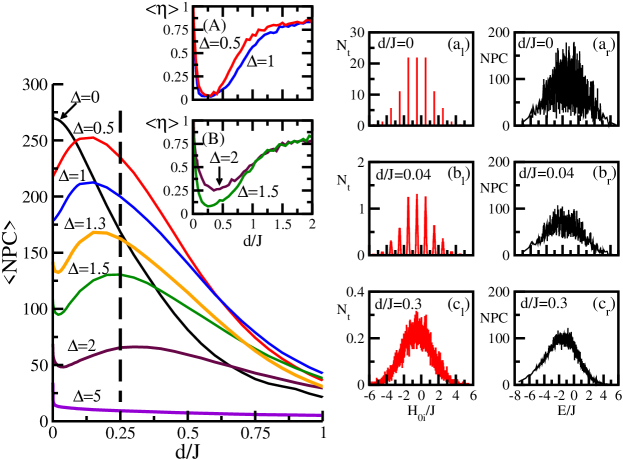
Figure 1: Interplay between interaction and uncorrelated random disorder. Main panel: NPC is the site-basis vs. $d/J$. Average over 924 states and 20 realizations. Panels (A) and (B): Level of chaoticity vs. $d/J$ (unfolding as described in  Santos (2004); not (b)); average over 20 realizations. Panels (a_l,r), (b_l,r), (c_l,r): $\Delta=2$; left: normalized histogram for the diagonal matrix elements $H_{0i}$ ($N_{t}$ is the number of states); right: NPC vs. eigenvalues; 20 realizations. All panels: $L=12$, $M=L/2$, Gaussian random numbers: $\alpha=0$.

To better understand the further delocalization of wavefunctions in interacting 1D systems when disorder is considered, we select the case where $\Delta=2$ and compare, for three values of $d/J$, the histograms of the diagonal elements $H_{0i}$ in panels a_l, b_l, c_l and the plots of the level of delocalization of the eigenvectors of Hamiltonian (1, 2) vs. their corresponding energies E in panels a_r, b_r, and c_r.

When $d/J=0$, the energies of the basis vectors form narrow bands of resonant states (a_l), the energies being determined by the number of pairs of neighboring excitations and by the number of excitations placed at the edges of the chain (border effects). These energies range from $-J\Delta(L-1)/4$ to $J\Delta(L-3)/4$ and the bands are separated by $J\Delta$. As the hopping term is turned on, only basis vectors belonging to the same symmetry sector can couple to form the wavefunctions. In addition, if $J\Delta>J$, the effects of $J$ on states belonging to different bands are negligible and the bands, although now of finite width, remain separated. In this case, only states placed in the same band and showing the same symmetries can mix, so the level of delocalization is reduced to the number of states in the band. Moreover, the number of states in a band decreases with the size of the clusters, that is, the number of neighboring excitations Kagan1984 . The overall effect in clean systems is therefore the monotonic decrease of average NPC with interaction. The right panel (a_r) shows the values of NPC. For this integrable system, no clear relationship between NPC and E is seen, as expected due to the absence of level repulsion. It is interesting to contrast this behavior with the 2D clean system, which is chaotic and outlines the shape typical of chaotic TBRE Kota (2001) already at $d/J=0$ (data not shown).

By slightly increasing $d/J$, the bands broaden. If $J\Delta>J$, they remain uncoupled (b_l): the number of resonant intra-band states then decreases and so does NPC (b_r). This explains the valley that precedes the peak in the NPC curves shown in the main panel. Larger disorder is then needed to overlap the bands (c_l) and increase delocalization (c_r). Notice that the average NPC for $d/J=0$ and 0.3 is approximately the same, although the NPC dependence on energy is significantly different (cf. a_r and c_r). The integrable clean chain shows no relationship between NPC and E (a_r), but as complexity increases and $\eta$ decreases, a relationship similar to those appearing in TBRE’s becomes evident (c_r): delocalized states are in the middle of the spectrum and only localized states appear in the edges.

The case of $\Delta=2$ is at the borderline, where band overlapping is significant and where level spacing distributions close to a Wigner-Dyson distribution may still be obtained. For larger interactions, such as $\Delta=5$, the bands are very separated at $d/J=0$ and do not merge together by increasing $d/J$, instead, larger disorder simply prevents resonances leading to the monotonic decay of NPC (see main panel).

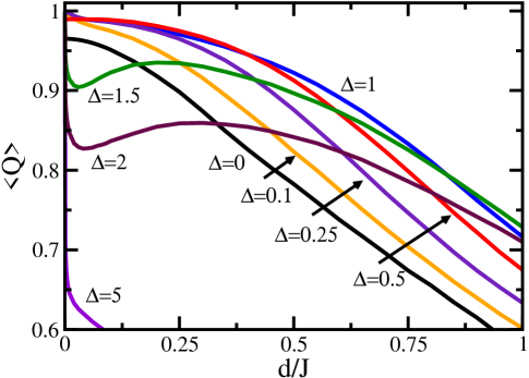
Figure 2: Interplay between interaction and uncorrelated random disorder. Average global entanglement vs. $d/J$. Average over 924 states and 20 realizations; $L=12$, $M=L/2$; $\alpha=0$.

Fig. 2 shows the behavior of global entanglement versus uncorrelated disorder for various values of the anisotropy not (c). A clean isotropic chain has $Q=1$, since the Hamiltonian is invariant under a global rotation of 180 degrees around the x-axis Brown et al. (2008). For $d/J\rightarrow 0$, contrary to NPC, the largest value of $Q$ is found for a clean system in the presence of weak interaction, $0<\Delta<1$. This suggests that interactions are key ingredients for the generation of non-local correlations in a half-filled chain. Therefore, we identify two main factors contributing for multipartite entanglement: the hopping term, which spreads the wavefunction [a state with on-site localization obviously shows no global entanglement], and the interaction term, which further enhances the correlations between the particles. High levels of entanglement require more than simply delocalization. As we discussed in Sec. II.E, it is possible to have very delocalized states with low entanglement.

Also in contrast with NPC, when $\Delta\leq 1$, global entanglement decreases monotonically with disorder. This is a result of the breaking of symmetries. It is possible, although this requires further investigation, that besides $S^{2}$ symmetry (and consequent rotational symmetry), reflection also has positive effects on quantum correlations. To illustrate this idea, compare the values of NPC and $Q$ in the table below. We have a system with $L=12$, $\Delta=0.5$, and two equal defects at the borders, $\omega_{1}=\omega_{L}=0.05J$, which guarantees that the $S^{2}$ symmetry is broken, but not parity. Suppose that we may include an additional defect on site $n$ with energy $0.5J$ (if $n=L$, then $\omega_{L}$ becomes $0.55J$). This is a simple way of breaking parity.

	NPC	$Q$
No additional defect	217	0.989
Additional defect at $n=L$	176	0.953
Additional defect at $n=(L/2)+1$	256	0.987

The chain with equal or unequal border defects is integrable Alcaraz1987 , whereas a defect in the middle leads to chaos Santos (2004). Independently of the position of the additional defect, it simply decreases $Q$. NPC, on the other hand, decreases only in the integrable regime, but increases in the chaotic region. It has been argued in Ref. Brown et al. (2008) that $Q$ seems closer related to NPC than with the integrable-chaos transition. Here, we go one step further and claim that, even though delocalization is necessary for the existence of quantum correlations, the two quantities do not always go hand in hand. The onset of chaos has a positive effect on spatial delocalization, whereas for global entanglement the breaking of symmetries associated with chaos are more detrimental than possible gains associated with further delocalization.

Large interactions ($\Delta>1$) are unfavorable to both NPC and $Q$, since the spectrum becomes gapped. However, for anisotropies not too large, $\Delta\gtrsim 1$, as $d/J$ increases and the energy bands overlap, the $Q$ curves quickly surpass the ones for smaller interactions. This reinforces once again the fundamental role of interactions in the creation of quantum correlations.

III.1.2 FP- and IP-basis

The results for NPC are entirely dependent on the basis chosen for the analysis. While the site basis is physically motivated by studies of spatial localization, further insight may be gained by considering alternative bases. To separate the regular motion dictated by integrable Hamiltonians from chaoticity, we show in Fig. 3 the behavior of delocalization vs. disorder for NPC computed in the FP- and IP-basis.

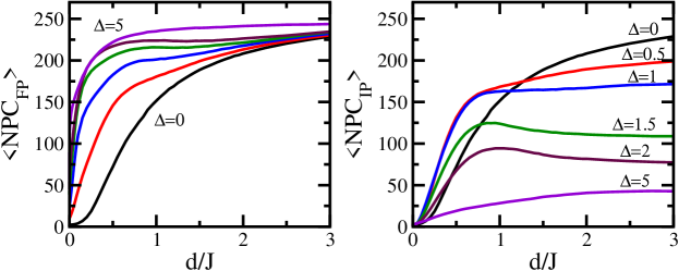
Figure 3: Average NPC vs. uncorrelated disorder. Left: NPC in the free-particle basis; from bottom to top: $\Delta=0,0.5,1,1.5,2,5$ Right: NPC in the basis of the integrable interacting clean chain. Average over 924 states and 20 realizations; $L=12$, $M=L/2$; $\alpha=0$.

The clean one-dimensional system considered here, with or without interactions, is integrable, chaos emerges only when disorder is added to it. In the FP-basis, a possible correlation between chaos and the complexity of the wavefunctions is reflected in the rate of delocalization, which increases abruptly in the chaotic region of $0<d/J<0.5$, $0<\Delta<1$, and is less dramatic for $\Delta=0$ and $\Delta>2$. But overall, NPC simply increases with $\Delta$. In contrast, in the IP-basis the behavior of NPC with $\Delta$ for $0<d/J<0.5$ is non-monotonic. Here, as in the site-basis case, delocalization is maximum where $\eta$ is minimum, the largest value appearing again for $\Delta=0.5$. It is only at large values of disorder that the behavior of NPC with $\Delta$ becomes trivial. Therefore, the effects of the interplay between interaction and disorder and the consequent onset of chaos are well singled out by the non-trivial behavior of NPC in both site- and IP-basis.

III.2 Long-range correlated random disorder

We now focus on a disordered chain with $d/J=0.25$ – the chaotic region of interacting systems – and proceed with a comparison between uncorrelated and correlated random disorder.

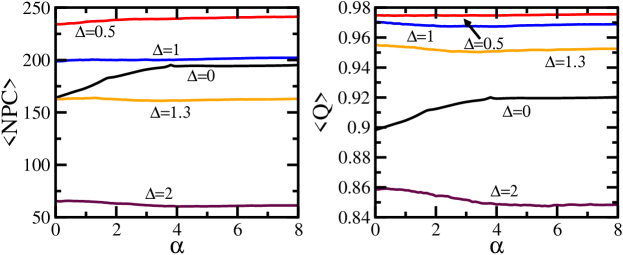
Figure 4: Interplay between interaction and long-range correlated random disorder. Left panel: Average delocalization in the site-basis vs. $\alpha$. Right panel: Average global entanglement vs. $\alpha$. All panels: $d/J=0.25$, $L=12$, $M=L/2$, average over 924 states and 20 realizations.

The left panel of Fig. 4 shows the average NPC vs. $\alpha$. The potential for spreading the wave functions associated with $\alpha>0$ has a non-monotonic behavior with the anisotropy. This may be explained as follows. Correlated disorder indicates more order, in a sense, it brings the system closer to a clean chain; but how the system approaches its clean limit is highly dependent on the interaction amplitude and the value of NPC we start with when $\alpha=0$. Long-range correlated disorder can always increase delocalization when $\Delta=0$, since a system with free particles is maximally delocalized in the absence of disorder (main panel in Fig. 1). The growth in NPC is obviously not sufficient to reach the values of a clean system, and not even those obtained for chaotic systems with $\Delta<1$, but, as shown in Fig. 4, it approaches the level of delocalization of a chaotic chain with $\Delta\sim 1$. For interacting systems, on the other hand, correlated disorder may decrease NPC. The maximum value of NPC when $\alpha=0$ depends on the amplitude of the uncorrelated disorder, $d/J$. When $d/J=0.25$ and $\alpha=0$, it is seen from the main panel in Fig. 1 that the NPC curves with $\Delta<1$ have already passed their maximum, while those with $\Delta\gtrsim 1$, such as $\Delta=2$, are right at their peak. Therefore, for $\Delta<1$, by increasing $\alpha$ we can further delocalize the system, whereas for $\Delta\gtrsim 1$, correlated disorder has the opposite effect of decreasing NPC. For large values of $\Delta$, such as $\Delta=5$, since NPC simply decays with uncorrelated disorder (main panel of Fig. 1), correlated disorder will always increase delocalization.

Insight on the non-trivial behavior of NPC with $\alpha$ may be gained by studying, in Fig. 5, how correlated disorder affects the histograms for the diagonal elements $H_{0i}$ and their consequences on the relation between NPC and the eigenvalues. We select four values of the interaction amplitude, $\Delta$ = 0, 0.5, 1.3, and 2.0.

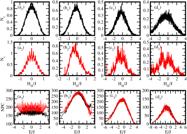
Figure 5: Uncorrelated vs. long-range correlated random disorder. First and second rows: normalized histograms for the diagonal matrix elements $H_{0i}$ with uncorrelated and correlated disorder, respectively. Third row: NPC vs. eigenvalues; black curve: $\alpha=0$; red curve: $\alpha=10$. Columns from left to right: $\Delta=0,0.5,1.3,2$. All panels: $L=12$, $M=L/2$, 40 realizations.

For uncorrelated disorder, as $\Delta$ increases, the distribution of $H_{0i}$ simply broadens (Fig. 5 a₁, b₁, c₁, d₁), however NPC does not decrease monotonically. As seen in the main panel Fig. 1, for $d/J=0.25$, $\Delta$ = 0 and 1.3 lead approximately to the same value of NPC, delocalization is maximum at $\Delta\sim 0.5$ and is very low for $\Delta=2$. This non-trivial behavior is associated with the transition to chaos from $\Delta=0$ to $\Delta=0.5$: The featureless curve of NPC vs. E (a₃), which shows intermediate values of delocalization for all energies, is substituted by a curve that peaks in the middle of the spectrum (b₃). As expected from chaotic TBRE’s, for $\Delta=0.5$, NPC approaches the GOE value of $N/3$ in the middle of the spectrum and has smaller values only at the edges. This results in an overall increase of $\langle$NPC$\rangle$. It is only from $\Delta=0.5$ to $\Delta=1.3,2.0$, that the broadening of the distributions of diagonal energies leads to the decrease of NPC (c₃,d₃).

The inclusion of random disorder with long-range correlation ($\alpha=10$) has little effect on the delocalization of a half-filled system with interacting particles, but it significantly affects the model with non-interacting particles. When $\Delta=0$, correlated disorder increases the number of resonances in the middle of the histogram (compare a₁ and a₂), leading to an interesting shaped distribution. This is reflected in the larger values of NPC in panel a₃. When $\Delta=0.5,1.3$, the shape of the distribution changes slightly (cf. b₁, b₂ and c₁, c₂), having little effect on the curves for NPC vs. E (b₃, c₃). However, when $\Delta=2$ the energy band overlapping obtained by adding uncorrelated disorder (see a_l, b_l, and c_l of Fig. 1 and d₁ here) is partially removed by adding order via $\alpha$ (d₂). This explains the decay of $\langle$NPC$\rangle$ verified in Fig. 4. The effects of correlated disorder are, however, limited and all curves for NPC and $Q$ saturate for $\alpha>4$ (see Fig. 4).

There are then two possibilities to increase delocalization in a chain of free particles with uncorrelated disorder: by including weak interaction, so that chaos may set in, or by pushing the system toward the clean limit by adding correlated on-site energies. The two alternatives constitute, however, opposite procedures, so when put together their effects do not add up.

In general, the behavior of multipartite entanglement and delocalization with correlated disorder are comparable. Similarly to NPC, the effects of $\alpha$ on $Q$ also depend on the value of $Q$ we start with when $\alpha=0$, an information extracted from Fig. 2. In the presence of correlated on-site energies, the right panel of Fig. 4 shows that (i) global entanglement increases with $\alpha$ when $\Delta=0$, (ii) $Q$ is not much affected by correlated disorder when $\Delta\sim 1$, (iii) $Q$ decreases with $\alpha$ when $\Delta\gtrsim 1$. Notice, however, the prominent role of interaction in establishing quantum correlations. In particular, compare the behavior of the curves for $\Delta=0$ and 1.3. When $\alpha=0$, NPC${}_{\Delta=0}\sim$ NPC_Δ=1.3, while $Q_{\Delta=1.3}\sim 1.06\;Q_{\Delta=0}$. When $\alpha=8$, NPC_Δ=0 increases significantly and becomes approximately 20% larger than NPC_Δ=1.3, while the growth of $Q_{\Delta=0}$ is more limited and it remains smaller than the global entanglement for $\Delta=1.3$, $Q_{\Delta=1.3}\sim 1.03\;Q_{\Delta=0}$.

IV Dilute Limit

The dilute limit implies $M\ll L$. Here, we focus on the smallest value of $M$ where the interaction plays a role, the two particle case, $M=2$, and study the competition between interaction and both uncorrelated and correlated disorder.

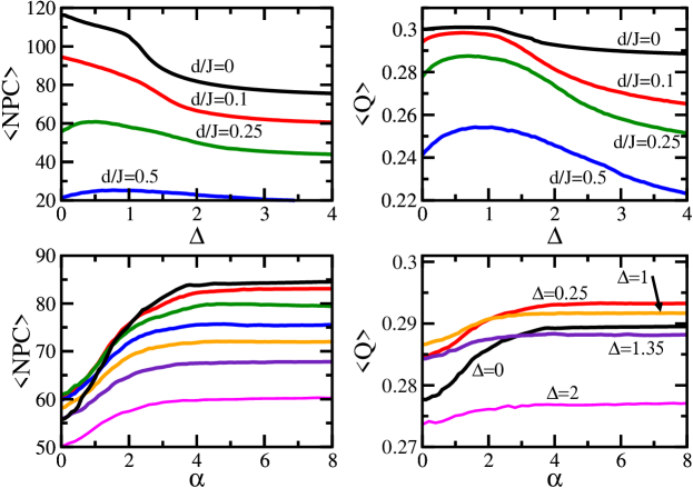
Figure 6: Top panels: interplay between interaction and uncorrelated disorder, $\alpha=0$; bottom panels: interplay between interaction and long-range correlated disorder, $d/J=0.25$. Top left (right) panel: Delocalization (Global entanglement) vs. anisotropy for different values of $d/J$. Bottom left (right) panel: Delocalization (Global entanglement) vs. $\alpha$ for different values of $\Delta$. Left bottom panel - curves from top to bottom at $\alpha=8$: $\Delta=0,0.25,0.5,0.75,1,1.35,2$. All panels: $L=24$, $M=2$, average over all states and 20 realizations.

From the top panels of Fig. 6, one sees that for a fixed value of the interaction amplitude, NPC and $Q$ decay monotonically with disorder. This justifies our choice here to consider $\Delta$ in the abscissa, instead of $d/J$, as in Figs. 1, 2. For $d/J\neq 0$, such as $d/J=0.25$ and 0.5, a value of $\Delta\neq 0$ may still exist where NPC and $Q$ become maximum, but the effects of the interaction are now much less prominent than in the half-filled chain. In the dilute limit, the $H_{XY}$ term dominates over the Ising interaction and becomes the main determining factor for the level of delocalization and global entanglement. As a result, the behaviors of NPC and $Q$ are more comparable than at half-filling (cf. Fig. 6 and Figs. 1, 2).

The bottom panels show how NPC and $Q$ behave with correlated disorder for various values of $\Delta$, keeping fixed $d/J=0.25$. Contrary to the half-filled case, for all cases considered here, NPC and $Q$ increase with $\alpha$. This is a reflection of the trivial behavior of NPC and $Q$ with uncorrelated disorder. Moreover, the effects of $\alpha$ are now more pronounced than in the half-filled chain, especially for the chain with $\Delta=0$. NPC_Δ=0 now surpasses all curves shown and even $Q_{\Delta=0}$ manages to outperform $Q_{\Delta=1.35}$. In comparison to the $M=L/2$ case, correlated disorder can now bring NPC and $Q$ closer to the values of a clean chain. These results simply reflect the minor role of the interaction in a dilute system. The increase of NPC_Δ=0 from $\alpha=0$ to $\alpha>4$ is more than 50% for $L=24$, $M=2$. As expected, this behavior is yet amplified in larger systems, as shown in the left bottom panel of Fig. 7.

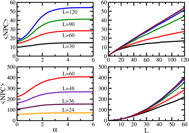
Figure 7: Effects of the chain size on delocalization in the presence of long-range correlated disorder. Top panels: $M=1$, bottom panels: $M=2$ and $\Delta=1$. Left panels: Delocalization vs. $\alpha$ for different values of $L$; right panels: Delocalization vs. chain size for different values of $\alpha$, curves from bottom to top: $\alpha=0,1,2,3,4,5$. Average over all states and 40 realizations.

The right panels of Fig. 7 compare delocalization with system size in the case of $M=1$ and $M=2$ for different values of $\alpha$. When $M=1$ the dimension of the Hamiltonian is $N=L$. For $\alpha=0$, as seen in the top right panel, apart from small system sizes where border effects are important, there is little difference between the NPC values for different $L$’s. This result is in agreement with the fact that Anderson localization occurs in one-dimensional systems with a single particle, that is, uncorrelated random on-site energies lead to a finite localization length of the wavefunctions. On the other hand, for large values of $\alpha$, the increase rate of NPC becomes linear. Large correlations between on-site energies bring the behavior of NPC closer to that of a clean system, where NPC $\propto L$. This is consistent with Ref. de Moura and Lyra (1998), where it was shown that, in the thermodynamic limit, one-particle states become delocalized for $\alpha>2$.

When $M=2$, the dimension of the Hamiltonian is quadratic on the system size, $N=L(L-1)/2$. In this case, as shown in the right bottom panel, NPC grows quadratically with $L$ even when $\alpha=0$. This suggests that, on average and for the finite systems studied here, there is no sign of Anderson localization for states with two interacting particles, even when the disorder is uncorrelated. There are, however, few isolated states with small NPC (data not shown), which accounts for situations where the particles are sufficiently apart, so that the interaction is negligible and the particles are individually localized. Further studies are now required to conclude if, on average, localized states will be the dominating scenario for larger chains, or if interaction will in fact prevent localization even in the thermodynamic limit.

V Discussion and Conclusion

We studied how delocalization and global entanglement in a quantum many-body one-dimensional system are affected by the interplay between on-site (uncorrelated and long-range correlated) random disorder and nearest-neighbor interaction. The analysis applies equally to a chain with spins-1/2, spinless fermions, or hard-core bosons. Half-filled and dilute chains were considered.

In a half-filled chain, the largest value of spatial delocalization (NPC) appears in a clean chain ($d/J=0$) with non-interacting particles ($\Delta=0$). Here, the only constraints in the spreading of the wavefunctions are the symmetries of the system and the boundary conditions. The addition of uncorrelated disorder to a non-interacting system or the inclusion of interaction to a clean chain, suppresses resonances and decreases NPC. On the other hand, when both $\Delta$ and $d/J$ are present, the behavior of NPC becomes non-trivial. A clean chain with interacting particles constitutes an integrable model with eigenvectors delocalized in the site-basis. As uncorrelated disorder is added, symmetries are broken. In the case of weak interaction, $0<\Delta\leq 1$, this leads to the onset of chaos and the further increase of NPC in the site-basis.

The behavior of global entanglement ($Q$) is influenced by delocalization, but does not follow it exactly. In particular, for $d/J\rightarrow 0$, the largest values appear in the presence of weak interaction. Also different, in weakly interacting systems, is its steady decay with uncorrelated disorder and the consequent breaking of symmetries. Besides delocalization, key contributing factors for global entanglement are then interactions and symmetries.

We have also briefly commented on the results for NPC in bases other than the site-basis. The latter is considered in studies of spatial localization, which was our main goal in this work. However, it is also useful to separate regular motion from chaoticity by analyzing delocalization in a basis where the model is integrable. In the basis consisting of eigenstates of a clean system with interaction (IP-basis), a non-monotonic behavior of NPC with $\Delta$ was also verified for disordered systems with $d/J<1$. This non-trivial behavior of NPC with interaction in both the IP- and the site-basis appears to be a main indication of the complexity enhancement of wavefunctions in the chaotic region.

The presence of correlated disorder ($\alpha\neq 0$) has different consequences depending on the value of $\Delta$. By correlating on-site energies, the level of order increases. A disordered system with non-interacting particles then gets closer to the limit of a clean chain and NPC increases. In the presence of interaction, the effect is opposite, since here it is disorder that enhances delocalization by breaking symmetries and overlapping energy bands. The behaviors of NPC and $Q$ with $\alpha$ reflect the non-trivial behavior of these quantities with $d/J$ when $\alpha=0$.

The study of a dilute system allows for the consideration of larger chains. In the presence of uncorrelated disorder, contrary to the one-particle case, on average, our results show no sign of Anderson localization in the finite systems considered. Long-range correlation delocalize both one and two-particle states.

In a future work, we intend to search for conclusive evidences for the absence (or not) of localization of two-interacting-particle states in systems with uncorrelated disorder. We also aim to study in details the effects of symmetries on non-local correlations. Another question worth investigation is how the integrable and chaotic regimes of the considered one-dimensional systems relate to different transport behaviors, namely diffusive or ballistic Santos (2008), and to the problem of thermalization Zelevinsky et al. (1996); Rigol et al. (2008). Also interesting would be the comparison of results with the Hubbard model and the inclusion of long-range interactions to the systems considered.

We hope that our theoretical results will motivate experimental verifications. Useful tools to simulate many-body effects in simplified models of condensed matter physics as the ones described here are optical lattices. They allow for control of the parameters of the system, such as the strength of interaction and the level of disorder Greiner and Fölling (2008).