Model- and calibration-independent test of cosmic acceleration
Abstract
We present a calibration-independent test of the accelerated expansion of the universe using supernova type Ia data. The test is also model-independent in the sense that no assumptions about the content of the universe or about the parameterization of the deceleration parameter are made and that it does not assume any dynamical equations of motion. Yet, the test assumes the universe and the distribution of supernovae to be statistically homogeneous and isotropic. A significant reduction of systematic effects, as compared to our previous, calibration-dependent test, is achieved. Accelerated expansion is detected at significant level ( in the 2007 Gold sample, in the 2008 Union sample) if the universe is spatially flat. This result depends, however, crucially on supernovae with a redshift smaller than 0.1, for which the assumption of statistical isotropy and homogeneity is less well established.
Keywords: classical tests of cosmology, dark energy theory, supernova type Ia
1 Introduction
The concordance model of cosmology is very successful in describing observations. It states that the universe consists of baryonic and cold dark matter as well as a cosmological constant, where the baryonic matter makes up only 5% of the content of the universe. The cosmological constant contributes 72% and thus causes an accelerated expansion at the present epoch. A large variety of other cosmological models have been proposed that come to similar results. Especially as soon as homogeneity and isotropy are assumed, each model states accelerated expansion of the universe when confronted with observational data.
If we are only interested in the question, whether the universe really expands accelerated, but not in the specific content of the universe, proposing and testing a certain cosmological model is not the appropriate approach. This question rather needs to be answered as model-independent as possible, i.e. without making any assumptions about the matter and energy content of the universe. The so-called kinematical approach does so by using special parameterizations of the deceleration parameter [1, 2, 3], the scale parameter [4], the Hubble rate [5], the dimensionless coordinate distance [6, 7] or different distance scales [8]. Other published methods are to expand into principle components [9] or to expand the jerk parameter into a series of orthonormal functions [10].
It is, however, even possible to avoid these kinds of parameterizations. In [11] we presented a model-independent test to quantify the evidence for accelerated expansion with the only assumption that the universe is homogeneous and isotropic. While versions of this test have already been proposed [12] and applied [13, 14] by other groups, we additionally considered calibration effects, quantified the evidence for accelerated expansion and studied systematic effects.
The crucial assumption in our test is the Copernican principle. It states that we are typical observers in the universe. Together with the observed isotropy of the cosmic microwave background, the Copernican principle implies that the universe is also homogeneous, the statement of the cosmological principle.
Although it seems to be consequent to adopt the cosmological principle for the analysis of supernovae, a critical reflection on it is in order. Most probes of the statistical isotropy use objects at rather high redshift, while nearby probes show significantly less evidence for statistical isotropy. For supernovae, this issue has been investigated recently in [15, 16]. Statistically significant violation of isotropy was found for supernovae at redshift [16]: The fluctuation of the Hubble rate on opposite hemispheres on the sky is about . This corresponds to an anisotropy of distance moduli of mag, which has to be compared to the effect of acceleration, which is about mag.
The statistical homogeneity of the universe is less well established than the statistical isotropy at high redshifts. Several observations indicate that the scale of statistical homogeneity is of the order of Mpc (e.g. from luminous red galaxies [17], but see also [18]). For supernovae it has been pointed out already many years ago that dropping the assumption of homogeneity, but keeping that of isotropy around one point, allows for excellent fits of the Hubble diagram without invoking dark energy [19, 20]. This does not come as a surprise, because spherically symmetric dust models (also called Lemaitre-Tolman-Bondi models) have two arbitrary free functions and if only supernovae are considered a perfect fit can be obtained. Thus instead of interpreting the supernovae Hubble diagrams as evidence for dark energy, one could question the Copernican principle. In our test, we assume statistical homogeneity and isotropy. We somewhat relax that assumption in a second step by excluding nearby supernovae from the test. We will demonstrate below, that the nearby supernovae at are crucial in the detection of cosmic acceleration.
In the following section, we will shortly summarize the basic concept and results of our test. In the present work, we slightly modify the test in order to avoid systematics due to calibration. The reason for those systematics is also explained in the next section. In section 3 the modified test is presented and applied to different data sets, including the recently published Union set [21], assuming a spatially flat universe. The cases of open and closed universes will be considered in section 4.
2 Calibration-dependent test
We consider the distance modulus
| (1) |
of supernovae type Ia (SN Ia), where the luminosity distance is given in units of Mpc. and are the apparent and absolute magnitudes, respectively. If is the distance modulus of the -th SN with redshift , one can define a new quantity
| (2) |
where is the distance modulus of a universe that neither accelerates nor decelerates, i.e. with deceleration .
The weighted average of the is given by
| (3) |
where . The include measurement errors and errors due to peculiar velocities. The standard deviation of this average is calculated by
| (4) |
with being the number of SNe that is averaged over.
Our null hypothesis is that the universe never expanded accelerated which implies
| (5) |
Note that this holds independently of the content of the universe and does not depend on the validity of Einstein’s equations. Thus if the observed value of is significantly larger than zero, the null hypothesis can be rejected. In that case, one can state that there must have been a phase of acceleration. However, this does not exclude a phase of deceleration. From (1) and (2) it follows that we need and in order to test the null hypothesis (5). There always exist values of and such that (5) is satisfied. Thus, these values have to be fixed by an independent calibration measurement. This is in contrast to model-dependent tests, where a combination of and is used as a fitting parameter.
In [11], we considered two SN Ia data sets (the Gold sample [22] and the ESSENCE set [23]), two different light-curve fitters (MLCS2k2 [24] and SALT [25]) and two different calibrations (the calibration presented by Riess et al. [26] and that given by Sandage et al. [27], which in the following will be referred to as Riess calibration and Sandage calibration, respectively). We calculated the averaged value over all SNe of a data set with a redshift and divided the result by its standard deviation , thus obtaining the evidence for accelerated expansion. Assuming a flat universe, the ESSENCE set using the MLCS2k2 fitter and the Sandage calibration gave the weakest evidence, namely . In the other cases the evidence is much larger and goes up to 17 for ESSENCE (SALT) in the Riess calibration. Thus, we observe enormous systematic effects for the different data sets, fitting methods and calibrations.
Consequently, we have to make an attempt to reduce these large systematics. It turns out that they are largely due to systematics in the calibration. This can be understood by the following considerations.
The absolute magnitude and the Hubble constant cannot be determined independently by only considering SNe. Thus, the absolute magnitude of the SNe Ia has to be calibrated by measurements of the distance moduli of cepheids in the host galaxies. Then SNe can be used to determine . As there is still some controversy between different groups about the correct calibration, we considered two very discrepant calibrations for our test of accelerated expansion. This test, however, does not depend on and independently, but on the quantity , which can be seen when we rewrite the null hypothesis as
| (6) |
The fact that we observe huge systematic errors depending on the considered calibration seems somewhat strange: Assume we have found two different values and for the absolute magnitude of SNe Ia by cepheid measurements. Using these results, two values and for the Hubble constant can be obtained by observations of nearby SNe. Although and , the resulting values and are equal by definition, if the same set of low redshift SNe and the same analysis is used for the determination of the Hubble constant.
For our test in [11], we adopted the values of and given by Riess et al. [26] and Sandage et al. [27]. As the two groups analysed different SNe and used different analysis pipelines, they obtained and which (combined with and ) did not lead to the same , but different values and .
Thus, the observed systematics are not due to a different determination of the absolute magnitude , but are caused by the systematic errors and the different SN data sets used in the measurement of .
While our approach is to test a null hypothesis, model-dependent tests fit special cosmological models or parameterizations to observational data. An essential difference between these two approaches is that we test an inequality, whereas model-dependent tests use an equality, which requires different analyses. Model-dependent tests are typically based on the minimization of , where is one of the model parameters . Then one can estimate the likelihood as a function of the parameters, which allows marginalization over . As in our test an inequality is tested, this kind of analysis is not suitable. We cannot use as a free parameter, since the null hypothesis (6) is always fulfilled for large enough . Thus for the test summarized in this section, needs to be calibrated.
3 Calibration-independent test
It is, however, easy to modify our test in such a way that we can avoid using a certain calibration of when testing the accelerated expansion. We just need to consider relative values of instead of absolute values, i.e. we use rather than , where is the average of using only nearby SNe of a data set. Thus, the null hypothesis now reads111Note that this hypothesis does not correspond to the hypothesis of a never acclererating universe tested by an observer at .
| (7) |
The standard deviation is obtained by adding the standard deviations of and in quadrature. In the following, we will assume a spatially flat universe. Open and closed universes will be considered in the next section.
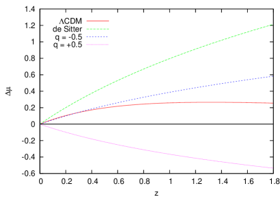
In figure 1a, is plotted for different spatially flat cosmological models: a CDM model with and (WMAP 5yr + BAO + SN best fit [28]), a de Sitter universe and models with constant deceleration (, which corresponds to the Einstein-de Sitter model) and constant acceleration (). Although the transition redshift between acceleration and deceleration in the CDM model is about , the curve still slightly increases beyond that redshift and has its maximum at . Thus, an increase of with redshift does not necessarily correspond to a phase of acceleration at that specific redshift. Note that for each value of the spatial curvature a different plot is necessary as in general depends on (see section 4).
Figure 1b shows averaged over redshift bins with width 0.2 for the Gold sample [22] (fitted with MLCS2k2), the ESSENCE set [23] (once fitted with MLCS2k2 and once with SALT) and the Union set [21] (fitted with SALT). As the first bin corresponds to the nearby SNe, its value is per definition equal to zero. The values in all the other bins are significantly above zero which indicates accelerated expansion. It is kind of a natural choice to define the nearby SNe as all SNe having a redshift smaller than 0.2 since at this point there is a gap in all presently available data sets. Doing so, there is a strong evidence for accelerated expansion.
Nevertheless, we also consider the cases where the nearby SNe are defined as those with and those with (figures 1c and 1d, respectively). In both plots a bin width of 0.1 is used. In figure 1d, the first bin is skipped and thus the second bin is fixed to zero. One can already see without any quantitative analysis that the evidence for acceleration dramatically decreases if SNe with are not used for the test. In particular for the two data sets that are fitted with MLCS2k2, the evidence completely vanishes since several data points become negative. However, one should not take that result very serious, as it is based on a very small number of SNe in the calibrating bin. Most reliable is the Union set with 6 SNe between redshift 0.1 and 0.2.
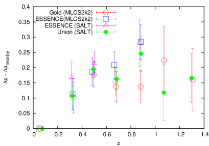
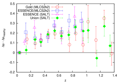
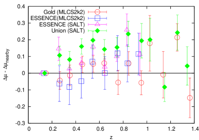
A quantitative value for the evidence of acceleration can be obtained by dividing by its standard deviation . The results corresponding to the bins plotted in figure 1 are given in table 1. A better statistics can be achieved when averaging over all SNe of a set with a redshift larger than that of the nearby ones. The results are listed in table 2. Although the test was only modified in order to avoid systematics from calibration, also the other systematics are reduced. In the test presented in [11] the calculated evidences varied from to in the Riess calibration and from to in the Sandage calibration. We then only used the Gold and ESSENCE sets, but not the Union set. For the same sets, using , we now obtain values that lie much closer to each other, namely between and .
-
Nearby SNe Bin Gold ESSENCE ESSENCE Union (MLCS2k2) (MLCS2k2) (SALT) (SALT) 2.0 2.2 3.2 3.5 4.4 4.2 5.2 6.8 2.8 4.6 3.4 4.4 2.6 4.9 3.7 4.2 2.0 1.3 1.6 2.1 2.8 2.2 3.8 0.6 1.8 2.2 3.4 2.9 2.0 2.0 2.2 2.8 3.9 2.9 4.0 5.3 3.9 5.3 4.8 5.2 3.7 4.2 2.5 3.3 1.1 5.2 5.1 3.6 2.8 3.7 3.7 3.8 1.1 3.5 1.7 2.2 1.9 1.8 0.9 0.7 4.3 2.7 0.1 0.6 0.8 0.6 2.1 1.9 0.2 0.8 0.5 1.7 1.1 0.5 1.9 3.5 1.1 0.7 3.3 3.8 1.1 0.0 0.7 2.4 0.8 1.1 3.3 2.7 0.8 0.5 2.7 3.1 0.8 0.9 0.9 1.9 1.1 1.6 0.1 1.0 2.6 2.3 1.2 0.4
-
Gold ESSENCE ESSENCE Union (MLCS2k2) (MLCS2k2) (SALT) (SALT) 4.3 5.2 5.6 7.2 4.4 5.7 5.7 5.9 0.8 0.9 4.3 3.7 #SNe at 36 43 44 51 #SNe at 4 4 2 6 #SNe at 142 115 132 250 #SNe in total 182 162 178 307
Analysing the data sets using and , respectively, a drawback of this test becomes evident: It crucially depends on the SNe in the first bin. (Note that this drawback is also implicitly included in calibration-dependent tests as nearby SNe are needed to determine and .) Skipping the SNe with a redshift smaller than 0.1, the evidence for acceleration vanishes if the MLCS2k2 fitter is used, which could be partly due to the fact that there are only four SNe classified as nearby. The reason why there is still some evidence if we use ESSENCE (SALT) instead of ESSENCE (MLCS2k2) is not only due to the systematic effects that occur when different light-curve fitters are used. The main reason is that there are only two nearby SNe in ESSENCE (SALT), which by chance have almost the same value of and thus a very small variance. The Union set contains 6 nearby SNe with and still states acceleration at .
As large scale structures are observed up to Mpc (the Sloan Great Wall [29]) which corresponds to a redshift of about , it is questionable if the assumption of isotropy and homogeneity is still justified for the analysis of SNe at lower redshifts. Thus, one should prefer to make cosmological tests using only SNe with higher redshifts and average over bin widths of at least . Unfortunately, this is not possible at the moment as there are very few SNe at redshifts between 0.1 and 0.3 in all presently available data sets. As soon as SN data at intermediate redshifts are published, repeating our analysis will show if better statistics gives rise to at least some evidence of cosmic acceleration and if there is still a significant difference in the evidences obtained by using MLCS2k2 and SALT, respectively.
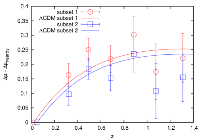
In order to analyse more quantitatively how much the evidence changes if the lowest redshifts are not considered, we split the SNe with of each set into two subsets containing an equal number of SNe. Subset 1 contains the SNe with the lowest redshifts, subset 2 those with the largest redshifts. is calculated using subset 1 and 2, respectively. For the determination of we use all SNe with . The result for the evidence for acceleration is shown in table 3. There is a tendency of decreasing evidence when the lowest redshift SNe are dismissed, which is not surprising. Only the Gold sample does not show this trend. The amount by which the evidence is decreased is, however, unexpected. This can be seen in figure 2 for the Union set: for a CDM model (, ) using subset 2 drops only by 0.018 mag as compared to the case when subset 1 is used, whereas the data points drop by 0.066 mag. Thus, the change in the data points is much larger than expected from CDM. A model with a steeper increase of at small redshifts would be more consistent with these data. An alternative explanation could be the so called Hubble bubble or large void scenario, i.e. the local value of could be different from the global one.
-
Gold ESSENCE ESSENCE Union (MLCS2k2) (MLCS2k2) (SALT) (SALT) subset 1 evidence 3.1 6.6 5.6 6.3 0.030 0.021 0.021 0.021 subset 2 evidence 3.4 3.2 3.9 4.8 0.056 0.046 0.050 0.051 # SNe 18 21 22 25
4 Open and closed universes
We now give up the assumption of spatial flatness. Then the distance modulus of a universe with deceleration parameter is given by
| (8) |
where for a closed and for an open universe. Using this, and subsequently can be easily calculated. Defining the nearby SNe as those with , the result for different values of the spatial curvature is given in table 4.
In a closed universe, decreases with increasing curvature, i.e. (and thus the evidence for accelerated expansion) increases. As we are interested in the lower limit of the evidence in a closed universe, we need to consider the smallest possible curvature, i.e. . Therefore, the results of the test are equal to those of a spatially flat universe. In an open universe the evidence decreases with increasing curvature. Thus, we need the largest possible value, , to determine the lower limit to the evidence. Note that is the largest possible curvature only if the rule holds, where . This rule is, however, only valid for general relativity and can be different in a modified gravity scenario. These weakest evidences for a flat/closed and an open universe are highlighted in table 4.
-
Gold ESSENCE ESSENCE Union (MLCS2k2) (MLCS2k2) (SALT) (SALT) closed universe 1.0 6.7 7.0 7.5 10.2 0.8 6.3 6.6 7.1 9.6 0.6 5.8 6.3 6.8 9.0 0.4 5.3 5.9 6.4 8.4 0.2 4.8 5.6 6.0 7.8 flat universe 0.0 4.3 5.2 5.6 7.2 open universe 0.2 3.8 4.9 5.3 6.6 0.4 3.3 4.5 4.9 6.0 0.6 2.8 4.1 4.5 5.4 0.8 2.3 3.7 4.1 4.8 1.0 1.8 3.4 3.8 4.2
5 Conclusion
We modified our model-independent test of accelerated expansion presented in [11] in such a way that systematics due to calibrations are avoided. This could be achieved by considering the SN data relative to the data in a bin of nearby SNe, where the most “natural” choice is to define the nearby SNe as those with redshift . Compared to the previous test, the evidence for acceleration is weaker, but all systematic effects are reduced. However, the evidence obtained from the ESSENCE set is still larger than that obtained from the Gold sample, and the SALT fitter gives a stronger evidence than MLCS2k2. Being conservative, one should take the lowest evidence obtained by using different data sets and light-curve fitters, i.e. 4.3 in the case of a spatially flat universe using the Gold sample fitted with MLCS2k2. The Union set is however not an independent data set, but contains SNe from Gold, ESSENCE and other sets. Thus, the Union set seems to be a good choice in order to determine the evidence for accelerated expansion. Unfortunately, the published data of this set have only been fitted with SALT. As for the ESSENCE set MLCS2k2 gives a weaker evidence than SALT, it is quite probable that this is also the case for the Union set. Then MLCS2k2 would give a more conservative value than the obtained 7.2 evidence.
By changing the set of nearby SNe, it becomes obvious that the test crucially depends on SNe with redshift . Skipping those data leads to vanishing evidence when the MLCS2k2 light-curve fitter is used. As a redshift of 0.1 corresponds approximately to a distance of 400Mpc, which is the size of the largest observed structures in the universe, the assumption of homogeneity and isotropy might not be justified for such low redshifts. For the Union set (based on 6 SNe between 0.1 and 0.2) still evidence is found. It remains to be seen if this is confirmed by larger data sets in the future.
We conclude that the largest publicly available supernova data sets show statistically significant evidence for cosmic acceleration if statistical isotropy and homogeneity are assumed at all redshifts. A violation of isotropy and/or homogeneity, e.g. by a local void, remains a viable alternative interpretation of supernova data (see e.g. [20]).
How to proceed? First of all we need more data at . This would allow to anchor our test with supernovae at intermediate redshifts, which should not be affected by the details of the local environment. Thus such a test could detect cosmic acceleration in a way that relies only on the assumptions of isotropy and homogeneity on scales at which they can be established by observations directly. Secondly, in [16] a significant anisotropy of Hubble diagrams on opposite hemispheres of the sky has been found. The direction of maximal asymmetry was found to be close to the pole of the equatorial coordinate system, which points towards systematic errors in existing data sets. Thus with improved data sets, especially better control on systematics at all levels, one could try to use SN Ia at to establish isotropy and homogeneity at even smaller redshifts. In both cases, ideally full sky surveys for nearby supernovae are required, while pencil beam like approaches would make it more difficult to disentangle a local void from dark energy.
References
References
- [1] Turner M and Riess A, Do SNe Ia provide direct evidence for past deceleration of the universe?, 2002 Astrophys. J. 569 18 [astro-ph/0106051]
- [2] Riess A et al., Type Ia supernova discoveries at from the Hubble Space Telescope: Evidence for past deceleration and constraints on dark energy evolution, 2004 Astrophys. J. 607 665 [astro-ph/0402512]
- [3] Elgarøy Ø and Multamäki T, Bayesian analysis of Friedmannless cosmologies, 2006 J. Cosmol. Astropart. Phys. JCAP09(2006)002 [astro-ph/0603053]
- [4] Wang Y and Tegmark M, Uncorrelated measurements of the cosmic expansion history and dark energy from supernovae, 2005 Phys. Rev. D 71 103513 [astro-ph/0501351]
- [5] John M, Cosmography, decelerating past, and cosmological models: Learning the bayesian way, 2005 Astrophys. J. 630 667 [astro-ph/0506284]
- [6] Daly R and Djorgovski S G, A model-independent determination of the expansion and acceleration rates of the universe as a function of redshift and constraints on dark energy, 2003 Astrophys. J. 597 9 [astro-ph/0305197]
- [7] Daly R, Djorgovski S G, Freeman K A, Mory M P, O’Dea C P, Kharb P and Baum S, Improved constraints on the acceleration history of the universe and the properties of the dark energy, 2008 Astrophys. J. 677 1 [arXiv:0710.5345]
- [8] Cattoën C and Visser M, Cosmographic Hubble fits to the supernova data, 2008 Phys. Rev. D 78 063501 [arXiv:0809.0537]
- [9] Shapiro C and Turner M, What do we really know about cosmic acceleration?, 2006 Astrophys. J. 649 563 [astro-ph/0512586]
- [10] Rapetti D, Allen S, Amin M and Blandford R, A kinematical approach to dark energy studies, 2007 Mon. Not. R. Astron. Soc. 375 1510 [astro-ph/0605683]
- [11] Seikel M and Schwarz D J, How strong is the evidence for accelerated expansion?, 2008 J. Cosmol. Astropart. Phys. JCAP02(2008)007 [arXiv:0711.3180]
- [12] Visser M, General relativistic energy conditions: The Hubble expansion in the epoch of galaxy formation , 1997 Phys. Rev. D 56 7578
- [13] Santos J, Alcaniz J, Pires N and Rebouças M, Energy conditions and cosmic acceleration, 2007 Phys. Rev. D 75 083523 [astro-ph/0702728]
- [14] Gong Y, Wang A, Wu Q and Zhang Y-Z, Direct evidence of acceleration from distance modulus redshift graph, 2007 J. Cosmol. Astropart. Phys. JCAP08(2007)018 [astro-ph/0703583]
- [15] Haugboelle T, Hannestad S, Thomsen B, Fynbo J, Sollerman J and Jha S, The velocity field of the local universe from measurements of type Ia supernovae, 2007 Astrophys. J. 661 650 [astro-ph/0612137]
- [16] Schwarz D J and Weinhorst B, (An)isotropy of the Hubble diagram: comparing hemispheres, 2007 Astron. Astrophys. 474 717 [arXiv:0706.0165]
- [17] Hogg D W, Eisenstein D J, Blanton M R, Bahcall N A, Brinkmann J, Gunn J E and Schneider D P, Cosmic homogeneity demonstrated with luminous red galaxies, 2005 Astrophys. J. 624 54 [astro-ph/0411197]
- [18] Labini F S, Vasilyev N L, Pietronero L and Baryshev Y V, The large scale inhomogeneity of the galaxy distribution, 2008 [arXiv:0805.1132]
- [19] Celerier M-N, Do we really see a cosmological constant in the supernovae data?, 2000 Astron. Astrophys. 353 63 [astro-ph/9907206]
- [20] Celerier M-N, The accelerated expansion of the universe challenged by an effect of the inhomogeneities. A review, 2007 [astro-ph/0702416]
- [21] Kowalski M et al., Improved cosmological constraints from new, old and combined supernova datasets, 2008 [arXiv:0804.4142]
- [22] Riess A et al., New Hubble Space Telescope discoveries of type Ia supernovae at : Narrowing constraints on the early behavior of dark energy, 2007 Astrophys. J. 659 98 [astro-ph/0611572]
- [23] Wood-Vasey W et al., Observational constraints on the nature of the dark energy: First cosmological results from the ESSENCE supernova survey, 2007 Astrophys. J. 666 694 [astro-ph/0701041]
- [24] Jha S, Riess A and Kirshner R, Improved distances to type Ia supernovae with Multicolor Light Curve Shapes: MLCS2k2, 2007 Astrophys. J. 659 122 [astro-ph/0612666]
- [25] Guy J, Astier P, Nobili S, Regnault N and Pain R, SALT: a Spectral Adaptive Light curve Template for type Ia supernovae, 2005 Astron. Astrophys. 443 781 [astro-ph/0506583]
- [26] Riess A et al., Cepheid calibrations from the Hubble Space Telescope of the luminosity of two recent type Ia supernovae and a re-determination of the Hubble constant, 2005 Astrophys. J. 627 579 [astro-ph/0503159]
- [27] Sandage A, Tammann G, Saha A, Reindl B, Macchetto F and Panagia N, The Hubble constant: A summary of the HST program for the luminosity calibration of type Ia supernovae by means of cepheids, 2006 Astrophys. J. 653 843 [astro-ph/0603647]
- [28] Komatsu E et al., Five-Year Wilkinson Microwave Anisotropy Probe (WMAP) observations: cosmological interpretation, 2008 [arXiv:0803.0547]
- [29] Gott J R I et al., A map of the universe, 2005 Astrophys. J. 624 463 [astro-ph/0310571]