Collisional decoherence in trapped atom interferometers that use non-degenerate sources

Abstract

The coherence time, and thus sensitivity, of trapped atom interferometers that use non-degenerate gases are limited by the collisions between the atoms. An analytic model that describes the effects of collisions between atoms in an interferometer is developed. It is then applied to an interferometer using a harmonically trapped non-degenerate atomic gas that is manipulated with a single set of standing wave laser pulses. The model is used to find the optimal operating conditions of the interferometer and direct Monte-Carlo simulation of the interferometer is used to verify the analytic model.

I Introduction

To date cold atom interferometers have demonstrated rotation sensitivities comparable to ring laser and mechanical gyroscopes Durfee et al. (2006). Several atom interferometer schemes have been realized, and thus far free space fountain and beam configurations, that utilize light pulses to manipulate the atoms, have demonstrated the greatest sensitivities Durfee et al. (2006); Peters et al. (1999); Hogan et al. (2008). While the lack of external potential reduces systematic errors, atom interferometry in free space is limited by acceleration due to gravity. In particular, the precision of an interferometer is directly proportional to the interrogation time and in free space this time is limited by the size of the vacuum chamber. In the most sensitive free space atom interferometers, the atomic clouds travel up to 10 meters Hogan et al. (2008). The large scale of free space interferometers limits their applications.

There is currently a great effort being made to reduce the size of atom interferometers while simultaneously increasing their sensitivity. One straightforward way to achieve this goal is to develop interferometers that trap the atoms in an external potential for the duration of the interferometer cycle. The external potential prevents the atoms from falling due to gravity, and keeps the atomic gas from expanding in the vacuum chamber. As a result, the interferometer cycle time is not as limited by the size of the chamber.

Several groups have built trapped atom interferometers using atomic gases that are both above and below the recoil temperature Schumm et al. (2005); Wang et al. (2005); Garcia et al. (2006); Horikoshi and Nakagawa (2006); Jo et al. (2007); Wu et al. (2007a). To date, all interferomters that use gases below the recoil temperature have utilized atoms in a nearly pure Bose-Einstein condensate (BEC).

If the gas is cooled below the recoil temperature and is split using a laser pulse, a large relative separation between each arm of the interferometer can be achieved Garcia et al. (2006). By exposing the atoms in each arm to a different environment, precision measurements of localized phenomena can be performed. For example, the AC stark shift in ${}^{87}\mbox{Rb}$ was recently measured by exposing the atoms in one arm of an interferometer to laser light Deissler et al. (2008).

In some applications, such as the sensing of rotations and accelerations, cloud separation is not necessary and interferomters that use non-degenerate source are sufficient. These sources can be produced by laser cooling alone. Additionally, non-degenerate atomic gases have a much lower density compared to a BEC and therefore experience a weaker mean-field potential. The mean-field potential directly couples number uncertainty into phase uncertainty via number dependent phase diffusion Jo et al. (2007); Javanainen and Wilkens (1997); Leggett and Sols (1998); Javanainen and Wilkens (1998). One advantage of working with laser cooled gases is that dephasing due to number fluctuations is ameliorated.

Besides the elimination of mean-field effects, atom interferometers that use laser cooled atomic gases are less sensitive to heating due to imperfections in the confining potential than a BEC. Atoms in a pure BEC experience no momentum changing collisions with other atoms in the same mode. Therefore, an interferometer that uses a pure BEC will experience little decoherence due to collisions. However, if a BEC is heated, atoms will leave the condensate and will experience an increase in the collision frequency. As a result, the decoherence rate will increase with temperature. On the other hand, if the interferometer uses a laser cooled gas with a temperature much greater than the BEC transition temperature, the density will decrease as the temperature increases and the decoherence rate will decrease if the gas is inadvertently heated.

Several different methods for building atom interferometers using laser cooled gases have been developed Cronin et al. (2007) and time-domain atom interferometers that use a single internal quantum state Cahn et al. (1997) lend themselves naturally for use with trapped atomic gases. This type of interferometer uses a series of optical standing waves to manipulate the external states of the atoms in the cloud. The interferometric cycle begins by loading an atomic cloud in a magneto-optical trap. The trap is switched off and the atomic cloud begins to fall due to gravity. At the time $t=0$, the cloud is illuminated with a short pulse from the standing wave laser field. Shortly after the pulse, the cloud has a density modulation with a period of $\lambda/2$, where $\lambda$ is the wavelength of the laser field. The density modulation then disappears because of the thermal motion of the atoms in the cloud. At the time $t=T$ the gas is illuminated with a second pulse. Due to the Talbot-Lau effect, there is an echo of the density modulation at the times $t=nT$, for integers $n\geq 2$. If the atomic cloud experiences a non-uniform potential during the interferometer cycle, the density echos will be shifted relative to the initial modulation. The shift in the phase of the modulation can be determined by reflecting a probe pulse from a single laser beam off of the echo. The phase of the reflected probe pulse is directly proportional to the phase shift in the density modulation. By interfering the reflected probe pulse with a reference beam, the interferometer’s signal can be read.

Recently, a trapped time domain atom interferometer was built by the group at Harvard Wu et al. (2007a). This interferometer used an atom wave guide to confine the atoms in the perpendicular directions while allowing them to freely propagate along the parallel direction. A series of standing wave laser pulses were applied to the atoms, such that the wave vectors of the lasers pointed along the free direction of the guide. The Harvard group demonstrated that it is possible to electronically move the wave guide back and fourth perpendicular to the free direction of the wave guide so that the arms of the interferometer enclose an area, making the interferometer sensitive to rotations Wu et al. (2007a).

A major difficulty with all trapped atom interferometers that use optical pulses is that the residual potential along the guide causes decoherence Horikoshi and Nakagawa (2007); Wu et al. (2007b); Burke et al. (2008); Stickney et al. (2008). The groups that have built BEC based interferometers have mitigated the decoherence by either using a double reflection geometry or using the classical turning points of the residual potential to reflect the atoms. The Harvard group has reduced the effects of the residual potential by using an interferometric cycles with several laser pulses Su et al. (2008). Although this multi-pulse scheme greatly increases the coherence time of the interferometer, it also reduces the number of atoms participating as well as reducing the area inclosed by the interferometer.

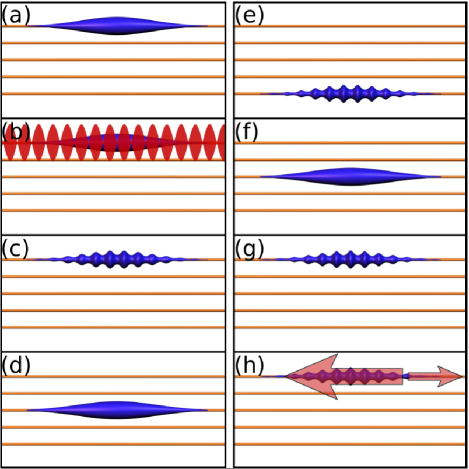
Figure 1: (color online) A schematic of the interferometer cycle. (a) The cold gas is loaded into a cigar shaped trap, created with the upper most horizontal wire (b) The atomic cloud is illuminated with a standing wave laser field. (c) After the laser pulse, a density modulation appears across the cloud. (d) The density modulation disappears and the trap is moved downwards by cycling the current in the wires. (e) The trap is above the bottom wire at a half period of the parallel trap and the density modulation reappears across the cloud. (f) The trap is moved upward and the density modulation disappears. (g) The trap reaches the top wire at one trap period of the parallel trap and the density modulation reappears for a second time. (h) A probe pulse is reflected off of the cloud.

We are currently developing a trapped atom gyroscope that uses a laser cooled atomic gas and avoids decoherence due to the residual potential by using classical turning points to reflect the atoms. Rather than utilizing the Talbot-Lau effect, the density modulation will echo twice every oscillation of the atoms in the parallel direction. Figure 1 is a schematic of the interferometer cycle. (a) Initially, a laser cooled atomic gas is loaded into a cigar shaped trap. The trap in the perpendicular direction is created with the upper most horizontal wire plus a uniform bias field. The relatively weak trap in the parallel direction is created using vertical wires that are not shown. (b) At the beginning of the interferometer cycle $t=0$, the atomic cloud is illuminated with a standing wave laser field. The atoms are accelerated towards the nodes of the laser field. (c) Immediately after the laser pulse, the atoms move towards the location of the nodes and density modulation appears across the cloud. (d) The density modulation disappears due to the thermal motion of the atoms. Simultaneously the trap is moved downwards by cycling the current in the wires. If the interferometer is rotating about the plane of the paper with frequency $\Omega$, the Coriolis force will accelerate the cloud in the parallel direction. (e) The cycling of the currents in the wires is timed so that the trap is above the bottom wire at half a period of the parallel trap $t=T/2$, where $T$ is the trap period in the parallel direction. Near $t=T/2$ there in an echo of the density modulation across the cloud. (f) The trap is moved upward. The Coriolis force decelerates the cloud resulting in a displacement of the cloud that is directly proportional to the rotation frequency of the interferometer. (g) At the time $t=T$, the trap returns to the top wire and there is a second echo of the density modulation. The modulation is shifted due to the rotation of the interferometer. The cycle (c) through (g) can be repeated many times. Since the oscillating Coriolis force is resonant with the parallel trap frequency, the shift in the displacement of the cloud will increase after each cycle. (h) After $n$ cycles, the displacement of the cloud is precisely measured by reflecting a probe beam off of the density modulation and interfering the reflected light with a reference beam.

The probe pulse only interacts strongly with the cloud when there is a density modulation across the cloud. As a result, the probe pulse can be longer than the duration of the modulation echo. Small fluctuations in the trap frequency can be measured simultaneously with the phase shift and using thermal atoms avoids the critical timing needed when a BEC is used Stickney et al. (2007); Horikoshi and Nakagawa (2007); Burke et al. (2008). It may prove possible to measure the interference signal more than once in any given experiment. As a result, it might be possible to split the atoms once, and measure the rotation frequency several times as the cloud oscillates in the trap.

During interferometer cycle, collisions between the trapped atoms will bring the gas back to equilibrium, causing a reduction in the amplitude of the density modulation. Thus, the amplitude of the reflected probe pulse will degrade with time. The upper limit on the interferometer cycle time and the devices sensitivity can be determined by analyzing the effects collisions between the atoms in the trap.

In this paper, we present a theoretical model for our interferometer. In Sec. II, we present an analytic model for the amplitude of the reflected probe pulse including the rotation of the interferometer and the effects of collisions between the atoms in the gas. In Sec. III the analytic model will be used to estimate the minimum value of the trap frequency in the perpendicular direction, the optimal temperature of the gas, and the optimal number of atoms to use in our upcoming experiment and we compare the results of our analytic model with a Direct simulation Monte-Carlo code. Finally Sec. IV conclusions will be presented.

II Formulation of the problem

The dynamics of a dilute atomic gas above BEC phase transition temperature is governed by the quantum Boltzmann equation Akhiezer and Peletminskii (1981)

$$\frac{d}{dt}\rho-\frac{1}{i\hbar}[H_{eff},\rho]=I(\rho),$$ (1)

where $\rho$ is the single particle density operator, $H_{eff}$ is the effective single particle Hamiltonian, and $I(\rho)$ is the collision integral. The effective Hamiltonian for an atom in a rotating trap and standing wave laser field is

$$H_{eff}=\frac{p^{2}}{2m}+V(\boldsymbol{r})+\hbar\chi\cos(2\boldsymbol{k}_{l}\cdot\boldsymbol{r})-\boldsymbol{\Omega}\cdot(\boldsymbol{r}\times\boldsymbol{p})+2U_{0}n(\boldsymbol{r}),$$ (2)

where $m$ is the atomic mass, $V$ is the external trapping potential, $\chi$ characterizes the strength of the standing wave laser, $\boldsymbol{k}_{l}$ is the wave vector of the laser field, and $\boldsymbol{\Omega}$ is the vector that points along the axes of rotation with the magnitude of the angular rotation frequency. The final term in Eq. (2) is the mean-field potential where $U_{0}=4\pi\hbar^{2}a_{s}/m$ characterizes strength of the atom-atom interactions, $a_{s}$ is the s-wave scattering length, and $n$ is the number density of the atomic gas. Note that the mean field potential for a non-condensed gas is a factor of two larger than for a BEC with the same density.

It is convenient to recast the single particle density operator in the Wigner function representation which is defined as

$$f(\boldsymbol{r},\boldsymbol{p})=\frac{1}{(\pi\hbar)^{3}}\int d^{3}r^{\prime}\langle\boldsymbol{r}-\boldsymbol{r}^{\prime}|\rho|\boldsymbol{r}+\boldsymbol{r}^{\prime}\rangle e^{2i\boldsymbol{r}^{\prime}\cdot\boldsymbol{p}/\hbar},$$ (3)

where $|\boldsymbol{r}\rangle$ are the eigenstates of the coordinate operator. The Wigner function can be interpreted as the probability density of finding an atom at the coordinate $\boldsymbol{r}$ with momentum $\boldsymbol{p}$.

It will be assumed that the standing wave laser pulse is in the Kapitza-Dirac regime. It is sufficiently short that both the free evolution of the gas and the collision integral may be neglected, i.e. the atoms do not move and experience no collisions while the laser beams are on. The pulse is in this regime when

$$\tau_{p}\ll\frac{\lambda}{\bar{v}},\tau_{p}\ll\frac{1}{\nu},$$ (4)

where $\tau_{p}$ is the length of the pulse, $\lambda$ is the wavelength of the laser beams, $\bar{v}$ is the average speed of the atoms in the gas, and $\nu$ is the average collision frequency. When Eq. (4) is fulfilled the dynamics of the atomic gas can be separated into two parts: the dynamics when the laser beams are on and the dynamics when the laser beams are off.

In what follows the dimensionless coordinate $\boldsymbol{r}^{\prime}=2k_{l}\boldsymbol{x}$, the dimensionless momentum $\boldsymbol{p}^{\prime}=\boldsymbol{p}/2\hbar k_{l}$ and the dimensionless time $t^{\prime}=t/t_{0}$ where $t_{0}=m/4\hbar k_{l}^{2}$ will be used. For ${}^{87}\mbox{Rb}$, the characteristic time is $t_{0}=5.3~{}\mu\mbox{s}$. Substituting Eq. (3) and (2) into Eq. (1) the dimensionless equation of motion for the Wigner function $f$, when the laser beams are on, is

$$\frac{\partial}{\partial t}f(\boldsymbol{r},\boldsymbol{p},t) = \chi\sin(2x)\left[f(\boldsymbol{r},\boldsymbol{p}-\boldsymbol{k}_{l}/2)-f(\boldsymbol{r},\boldsymbol{p}+\boldsymbol{k}_{l}/2)\right],$$ (5)

where $\boldsymbol{k}_{l}^{\prime}=\boldsymbol{k}_{l}/k_{l}$ is the direction of the standing wave laser field, $\chi^{\prime}=t_{0}\chi$ is the dimensionless laser strength, and all of the primes have been dropped. Similarly, the dimensionless equation of motion for the Wigner function $f$, when the laser beams are off, is

$$\frac{\partial}{\partial t}f(\boldsymbol{r},\boldsymbol{p},t) = -{\boldsymbol{p}}\cdot\frac{\partial f}{\partial\boldsymbol{r}}+\frac{\partial V_{eff}}{\partial\boldsymbol{r}}\cdot\frac{\partial f}{\partial\boldsymbol{p}}$$ (6)

$$- \boldsymbol{\Omega}\cdot\left(\boldsymbol{r}\times\frac{\partial f}{\partial\boldsymbol{r}}+\boldsymbol{p}\times\frac{\partial f}{\partial\boldsymbol{p}}\right)+I_{coll},$$

where $\Omega^{\prime}=t_{0}\Omega$, $y_{0}^{\prime}=2k_{l}y_{0}$ and once again all the primes have been dropped. Our short term goal is to measure the rotation of the Earth. For ${}^{87}\mbox{Rb}$ the rotation frequency of the Earth in our dimensionless units is $\Omega_{E}=4\times 10^{-10}$. When the gas is in thermodynamic equilibrium, the dimensionless temperature is $T^{\prime}=T/4T_{R}$, where $T_{R}=\hbar^{2}k_{l}^{2}/mk_{B}$ is the one photon recoil temperature. For ${}^{87}\mbox{Rb}$, the recoil temperature is $T_{R}=350~{}\mbox{nK}$.

The dimensionless effective potential is

$$V_{eff}=V+2gn,$$ (7)

where $V^{\prime}=t_{0}V/\hbar$ is the dimensionless trapping potential, $n^{\prime}=8k_{l}^{3}n$ is the dimensionless density, and $g=8\pi a_{s}k_{l}$ is the dimensionless mean-field strength. For ${}^{87}\mbox{Rb}$ the dimensionless mean-field strength is $g\sim 1$.

The length scale $L$ of density changes in a magnetically trapped atomic gas is typically much larger than the atoms s-wave scattering length $a_{s}$, i.e. $a_{s}/L\ll 1$. In this limit, the collision integral becomes independent of the potential. Since the atomic gas is above the BEC transition temperature, no single quantum state has a macroscopic population and Bose enhanced scattering can be neglected. The dimensionless collision integral can be approximated with the classical collision integral Akhiezer and Peletminskii (1981)

$$I_{coll}=\frac{\sigma}{4\pi}\int d^{3}p_{3}d\Omega|\boldsymbol{p}_{3}-\boldsymbol{p}|\left[f(\boldsymbol{r},\boldsymbol{p}_{1})f(\boldsymbol{r},\boldsymbol{p}_{2})-f(\boldsymbol{r},\boldsymbol{p}_{3})f(\boldsymbol{r},\boldsymbol{p})\right],$$ (8)

where $\sigma=32\pi a_{s}^{2}k_{l}^{2}$ is the dimensionless collision cross section. For ${}^{87}\mbox{Rb}$ the dimensionless scattering cross section is $\sigma=0.2$.

Before the laser pulse is applied, the gas is in thermodynamic equilibrium and it will be assumed that the laser pulse is sufficiently weak that the gas is always close to equilibrium. The Wigner function $f$ can be written as

$$f=f_{0}+\delta f,$$ (9)

where $f_{0}$ is the equilibrium Wigner function and $\delta f$ is the disturbance caused by the laser pulse. When the disturbance is much smaller than the equilibrium $|\delta f|\ll|f|$, Eq. (8) can be approximated as Chpman and Cowling (1970)

$$I_{coll}=\frac{\sigma}{4\pi}\int d^{3}p_{3}d\Omega|\boldsymbol{p}_{3}-\boldsymbol{p}|\left[2f_{0}(\boldsymbol{r},\boldsymbol{p}_{1})\delta f(\boldsymbol{r},\boldsymbol{p}_{2})-f_{0}(\boldsymbol{r},\boldsymbol{p}_{3})\delta f(\boldsymbol{r},\boldsymbol{p})-f_{0}(\boldsymbol{r},\boldsymbol{p})\delta f(\boldsymbol{r},\boldsymbol{p}_{3})\right].$$ (10)

Equation (10) is the sum of three terms, each with a simple physical interpretation. The first term $2f_{0}(\boldsymbol{r},\boldsymbol{p}_{1})\delta f(\boldsymbol{r},\boldsymbol{p}_{2})$ is proportional to the rate that an atom in $f_{0}$ scatters with an atom in $\delta f$ and one of the atoms scatters into the momentum state $\boldsymbol{p}$. The second term $f_{0}(\boldsymbol{r},\boldsymbol{p}_{3})\delta f(\boldsymbol{r},\boldsymbol{p})$ is proportional to the rate that atoms scatter out of $\delta f$ because of collisions with atoms in $f_{0}$. The final term $f_{0}(\boldsymbol{r},\boldsymbol{p})\delta f(\boldsymbol{r},\boldsymbol{p}_{3})$ is the inverse of the second process.

Only atoms in the disturbance contribute to the interference signal. Therefore, once an atom scatters out of the disturbance it no longer contributes to the interference signal. As a result only the second term in Eq (10) contributes to the loss of the interference signal and the collision integral Eq. (10) becomes

$$I_{coll}=\nu(\boldsymbol{r},\boldsymbol{p})(f_{0}(\boldsymbol{r},\boldsymbol{p})-f(\boldsymbol{r},\boldsymbol{p})),$$ (11)

where the collision frequency $\nu$ is given by the integral

$$\nu(\boldsymbol{r},\boldsymbol{p})=\sigma\int d^{3}p_{3}|\boldsymbol{p}_{3}-\boldsymbol{p}|f_{0}(\boldsymbol{r},\boldsymbol{p}_{3}).$$ (12)

Substituting the equilibrium distribution

$$f_{0}=\frac{1}{(2\pi T)^{3/2}}n(\boldsymbol{r})e^{-p^{2}/2T}$$ (13)

into Eq. (12), the collision frequency Eq. (12) becomes

$$\nu=\frac{2}{\pi}\rho(\boldsymbol{r})\sigma T^{1/2}K(|\boldsymbol{p}|/\sqrt{2T}),$$ (14)

where

$$K(\xi)=\int d\eta d\theta\eta^{2}\sin\theta\sqrt{\xi^{2}+\eta^{2}-2\xi\eta\cos\theta}e^{-\eta^{2}}.$$ (15)

The integral $K(\xi)$ can be explicitly evaluated in terms of error functions. To remove the dependnce of $\nu$ on the coordinate $\boldsymbol{r}$ and momentum $\boldsymbol{p}$, Eq. (15) will be replaced by its value a zero argument $K=1$ and the density $n$ will be replaced by the averaged density of a gas thermodynamic equilibrium in a harmonic potential. The collision frequency Eq. (12) becomes

$$\nu=\frac{2^{1/2}}{(2\pi)^{2}}\frac{\bar{\omega}^{3}\sigma N}{T},$$ (16)

where $\bar{\omega}=(\omega_{\parallel}\omega_{\perp}^{2})^{1/3}$ is the geometric average of the trap frequencies. In Sec. III it will be demonstrated that using Eq. (16) for the collision frequency yields accurate results when compared to a more complete description of the atomic collisions.

For the rest of this paper, we will limit the discussion to the case of a cigar shaped harmonic potential. The dimensionless trapping potential becomes

$$V=\frac{1}{2}\left\{\omega_{\parallel}^{2}x^{2}+\omega_{\perp}^{2}\left[(y-y_{0})^{2}+z^{2}\right]\right\},$$ (17)

where $\omega_{\perp}^{\prime}=t_{0}\omega_{\perp}$ and $\omega_{\parallel}^{\prime}=t_{0}\omega_{\parallel}$. If the trap has frequencies $\omega_{\parallel}=2\pi\times 3~{}\mbox{Hz}$ and $\omega_{\perp}=2\pi\times 300~{}\mbox{Hz}$, the dimensionless trap frequencies for ${}^{87}\mbox{Rb}$ are $\omega_{\parallel}^{\prime}=10^{-4}$ and $\omega_{\perp}^{\prime}=10^{-2}$.

When the gas is close to thermodynamic equilibrium in a harmonic trap the density is

$$n=\frac{N\bar{\omega}^{3}}{(2\pi T)^{3/2}}e^{-V/T},$$ (18)

where $N$ is the number of atoms in the trap and $V$ is the potential. Using Eq. (7) and (18) the effective potential can be expanded to fourth order as

$$V_{eff}=\left(1-\frac{2g\bar{\omega}^{3}N}{(2\pi T)^{3/2}}\right)V+\frac{2g\bar{\omega}^{3}N}{(2\pi)^{3/2}T^{7/2}}V^{2}.$$ (19)

The lowest order mean field contribution to the potential causes a small reduction of the trap frequency. Therefore, the oscillation period of atoms in the trap is weakly dependent on the number of trapped atoms. The next higher order contribution is a weak quartic contribution to the potential. This, and all higher order terms, can be neglected when

$$\frac{2g\bar{\omega}^{3}N}{(2\pi)^{3/2}T^{7/2}}\ll 1.$$ (20)

For example if the trap contains $7\times 10^{6}$ ${}^{87}\mbox{Rb}$ atoms, in a trap with frequencies $\omega_{\parallel}=2\pi\times 3~{}\mbox{Hz}$ and $\omega_{\perp}=2\pi\times 300~{}\mbox{Hz}$, and a temperature of $40~{}\mu\mbox{K}$ ($T=30$), the left hand side of Eq. (20) is about $6\times 10^{-8}$. In this case, the quantric contribution to the potential can be neglected.

The analysis of the operation of the interferometer will be limited to the case where the splitting and read lasers beams are aligned with the weak axis of the harmonic potential, which will be chosen to be the $x$ direction. For definiteness, the rotation of the interferometer will be in the $z$ direction and the trap will be moved in the $y$ direction. An atomic cloud at temperature $T$ remains in equilibrium if the center of the trap is translated adiabatically. The trajectory of the moving trap $y_{0}(t)$ is adiabatic when

$$\frac{d^{2}y_{0}}{dt^{2}}\ll\sqrt{T}\omega_{\perp},$$ (21)

where $\omega_{\perp}$ is the trap frequency in the $y$ direction.

When Eq. (21) is fulled, the equations of motion Eq. (5) and (6) can be recast in a one-dimensional form. The Wigner function is written as the product $f(x,r_{\perp},p,p_{\perp})=f(x,p)F(r_{\perp},p_{\perp})$, where $F(r_{\perp},p_{\perp})$ is the equilibrium distribution in the perpendicular direction, normalized to one, and $f(x,p)$ is the non-equilibrium distribution in the parallel direction, normalized to the number of atoms in the trap. When the laser beams are on, the one-dimensional equation of motion for the Wigner function is

$$\frac{\partial f}{\partial t}=\chi\sin(x)\left[f(x,p-1/2)-f(x,p+1/2)\right],$$ (22)

The solution of Eq. (22) can be written in terms of Bessel functions of the first kind $J_{\nu}$,

$$f(x,p,t)=\sum_{lk}(-i)^{l}J_{k}(\Xi)J_{l+k}(\Xi)e^{i(l+2k)x}f_{0}(x,p-l/2),$$ (23)

where the sum over $k$ and $l$ runs from $-\infty$ to $\infty$, $\Xi=\int dt^{\prime}\chi(t^{\prime})$ is the strength of the laser pulse, and

$$f_{0}=\frac{N\omega_{\parallel}}{2\pi T}\exp\left[\frac{p^{2}+\omega_{\parallel}^{2}x^{2}}{2T}\right]$$ (24)

is the equilibrium Wigner function at temperature $T$. In general Eq. (23) can be negative, because the resulting gas is in a non-classical state. However, for high temperatures $T\gg 1$ the negative parts of the Wigner function are negligible, and the gas may be treated classically.

After the laser pulse is applied, the optical field is turned off and the one-dimensional equation of motion for the Wigner function becomes

$$\left[\frac{\partial}{\partial t}+(p-\Omega y_{0})\frac{\partial}{\partial x}+\omega_{\parallel}^{2}x\frac{\partial}{\partial p}\right]f=\nu(f_{0}-f),$$ (25)

where the collision frequency $\nu$ is given by Eq. (16). The left hand side of Eq. (25) can be greatly simplified by introducing the new coordinates

$$x^{\prime} = x\cos\omega_{\parallel}t-\frac{p}{\omega_{\parallel}}\sin\omega_{\parallel}t+\Omega\int^{t}d\tau y_{0}(\tau)\cos\omega_{\parallel}\tau$$

$$p^{\prime} = \omega_{\parallel}x\sin\omega_{\parallel}t+p\cos\omega_{\parallel}t+\Omega\omega_{\parallel}\int^{t}d\tau y_{0}(\tau)\sin\omega_{\parallel}\tau$$

$$t^{\prime} = t.$$ (26)

In this new coordinate system, Eq. (25) becomes

$$\frac{\partial}{\partial t}f=\nu(f_{0}-f),$$ (27)

which has the general solution

$$f(t)=f(0)e^{-\nu t}+f_{0},$$ (28)

where $f(0)$ is the initial Wigner function given by Eq. (23), $f_{0}$ is the equilibrium Wigner function given by Eq. (24), and $\nu$ is given by Eq. (16).

To read out the accumulated phase, the atomic cloud is illuminated with a single off resonate laser beam. The light that is back scattered off of the cloud is mixed with a reference beam Cahn et al. (1997); Wu et al. (2007b). By measuring the interference intensity, the amplitude of the scattered light can be determined. Using the Born approximation, it can be shown that the amplitude of the back scattered light is proportional to Wu et al. (2007b)

$$S=\int dxdpe^{ix}f(x,p),$$ (29)

where $f$ is the one-dimensional Wigner function. The quantity $S$ will be referred to as the interference signal of the interferometer.

In the new coordinate system Eq. (26), the signal becomes

$$S=e^{-i\varphi}\int dxdpe^{i(x\cos\omega t+p/\omega\sin\omega t)}f$$ (30)

where

$$\varphi=\Omega\left(\cos\omega t\int^{t}dt^{\prime}y_{0}(t^{\prime})\cos\omega t^{\prime}+\sin\omega t\int^{t}dt^{\prime}y_{0}(t^{\prime})\sin\omega t^{\prime}1\right)$$ (31)

is the phase shift due to the rotation of the interferometer.

Substituting Eq. (28) into Eq. (30) yields

$$S = Ne^{-i\varphi}\left\{\sum_{nk}(-i)^{n}J_{k}J_{n+k}e^{-\frac{T}{2\omega^{2}}\left[(\cos\omega t+n+2k)^{2}+\sin^{2}\omega t\right]+i\frac{n}{2\omega}\sin\omega t-\nu t}+e^{-T/2\omega^{2}}\right\}.$$ (32)

The interference signal $S$ is only nonzero when $t\approx 2n\pi/\omega$, where $n$ is an integer or half integer. Expanding Eq. (32) near these points and taking the limit where $T\gg\omega^{2}$ yields

$$S=-2Ne^{-i\varphi-T\tau^{2}/2-\nu t}\sum_{k=0}^{\infty}J_{k}J_{k+1}\sin((k+1)\tau/2)$$ (33)

where $\tau=t-2n\pi/\omega_{\parallel}$. Equation (33) along with Eq. (16) and (31) are the main analytical results of this paper.

III Discussion

Equation (33) will now be analyzed and optimal operating conditions for trapped thermal atom interferometers will be found. Additionally to confirm the results of the analytic model we will use a direct simulation Monte-Carlo model (DSMC) of the interferometer Garcia (2000).

Direct simulation Monte-Carlo is accurate because the equation of motion after the laser pulse Eq. (6) is equivalent to the classical Boltzmann equation. Since the effect of the standing wave laser pulse on the cloud is non-classical (Eq. (22) ), DSMC can only be used to model the dynamics when the standing wave laser beams are off. To account for the laser pulse, the initial conditions for the DSMC model was set by Eq. (23). In regions where the initial Wigner function is negative $f<0$, the classical distribution of atoms was set to zero. This is valid when the temperature is much larger than the two-photon recoil temperature $T\gg 1$.

For definitiveness, we specialize to the case where the trap is moved back and fourth according to

$$y_{0}=\frac{d}{2}\cos(\omega_{\parallel}t),$$ (34)

where $d$ is the dimensionless distance that the atomic cloud is displaced in the $y$-direction. Our chip will displace the trap about $5~{}\mbox{mm}$, for ${}^{87}\mbox{Rb}$ the dimensionless displacement will be $d=8\times 10^{4}$.

After $n/2$ oscillations, the atoms scattered into the first order will enclose an area $\pi nd/\omega_{\parallel}$ and the accumulated phase shift is

$$\varphi=\frac{\pi nd}{\omega_{\parallel}}\Omega.$$ (35)

To measure the rotation rate of the Earth, with a $\pi$ phase shift in a trap with $\omega_{\parallel}=2\pi\times 3~{}\mbox{Hz}$, the trap must be moved back and forth three times. The time that it takes for the interferometer to measure a given phase shift does not depend on the parallel trap frequency. For example the time that it takes to measure a $\pi$ phase shift $t_{\pi}$ is

$$t_{\pi}=\frac{4\pi}{\Omega d}.$$ (36)

To measure Earth’s rotation, with a $\pi$ phase shift, the interferometer must have a cycle time of about one second. To measure a given rotation frequency, the bandwidth of the interferometer can only be increased by increasing the distance that the atoms are displaced $d$. For the remainder of this paper only the interference signal will be discussed for the case where the phase shift $\varphi$ is zero and when the trap is not moved in the $y$-direction.

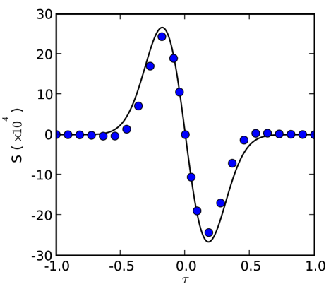
Figure 2: (color online) The interference signal as a function of time near one trap period. The solid curve is Eq. (33) and the dots are the results of the DSMC code.

Figure 2 shows the interferometer signal $S$, which is proportional to amplitude of the back scattered light, as a function of time. The sold line in Fig. 2 is Eq. (33) for times close to the first oscillation period $\tau=t-2n\pi/\omega_{\parallel}$ where $n=1$, and with the parameters $\sigma=0.2$, $\omega_{\perp}=10^{-4}$, $\omega_{\parallel}=10^{-2}$, $\varphi=0$, $N=7\times 10^{6}$, $\Xi=1$ and $T=30$. The dots are the result of the DSMC, with each super particle representing 10 atoms and the signal averaged over $64$ separate runs of the DSMC code. The error bars in all DSMC calculations are smaller than the size of the dots shown in the figures. This figure demonstrates good agreement between the analytic result and our DSMC code.

The shape of this signal illustrates the time and position varying amplitude of the density modulation echo relative to the probe laser. For times slightly less than one trap period $\tau<0$, the nodes of the density modulation are located at the anti-nodes of the standing wave laser field. At precisely one trap period, the density modulation vanishes and the cloud returns to its initial density distribution. For times slightly larger than one trap period $\tau>0$, the nodes of the density modulation are located at the nodes of the standing wave laser field.

For weak pulses $\Xi\lesssim 1$, the interference signal Eq. (33) can approximately written as

$$S=-A\tau e^{-T\tau^{2}/2-2n\nu\pi/\omega_{\parallel}},$$ (37)

where $A=N\sum_{k}J_{k}J_{k+1}(k+1)$. The two peaks in the signal occurs at the times $\tau=\pm T^{-1/2}$. For ${}^{87}\mbox{Rb}$ at $40~{}\mu\mbox{K}$ the time between the maximum and minimum signal is about $1~{}\mu\mbox{s}$. The magnitude at the peaks in the signal is

$$S_{peak}=A\frac{N}{T^{1/2}}\exp\left(-\frac{\omega_{\perp}^{2}\sigma Nn}{2^{1/2}\pi T}-\frac{1}{2}\right),$$ (38)

where Eq. (16) was used. For the remainder of this section, Eq. (38) will be analyzed for several illustrative cases. Using this analysis, limits on the performance of the interferometer will be discussed.

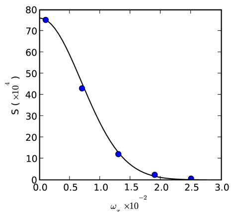
Figure 3: (color online) The maximum value of the interference signal as a function of perpendicular trapping frequency. The solid curve is found using Eq. (38) and the dots were extracted from a DSMC calculation.

Figure 3 shows the maximum value of the interference signal as a function of perpendicular trapping frequency $\omega_{\perp}$, where all the other parameters are the same as in Fig. 2. The solid curve is found using Eq. (38) and the dots were extracted from the DSMC calculation. This figure demonstrates excellent agreement between the analytic and DSMC models of the interferometer. The maximum interference signal is observed for small values of the perpendicular trapping frequencies. This is because the density of the atoms decreases as the atoms are confined less tightly in the perpendicular direction.

From Fig. 3, it is clear that the optimal value of perpendicular trapping frequency is the smallest value such that the movement of the trap remains adiabatic. The minimum transverse trap frequency can be estimated by using Eq. (21) and (34). To remain adiabatic, the ratio between the transverse and perpendicular trapping frequencies must be

$$\frac{\omega_{\perp}}{\omega_{\parallel}}\gg\frac{\omega_{\parallel}d}{2\sqrt{T}},$$ (39)

where $d$ is the maximum displacement of the trap in the perpendicular direction and $T$ is the temperature of the gas.

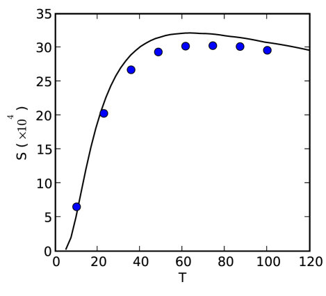
Figure 4: (color online) The maximum value of the interference signal as a function of temperature. The solid curve is Eq. (38) and the dots were extracted from a DSMC calculation.

Figure 4 shows the maximum value of the interference signal as a function of the temperature $T$ of the trapped gas. The remaining parameters are the same as Fig. 2. The solid curve is Eq. (38) and the dots were extracted from the DSMC calculation. There is still good agreement between the analytic and DSMC models.

Holding all other parameters constant, the interference signal becomes smaller as the temperature is reduced. This is because, in a harmonic potential, collision rate is inversely proportional to temperature. For the parameters used in Fig. 4, the signal increases with temperature until $T=60$. For temperatures larger than $T>60$, the duration of the echo becomes shorter and the amplitude of the density modulation is reduced. Using Eq. (38) it can be shown that the largest amplitude of back-scattered light occurs when the temperature is

$$T=\frac{2^{1/2}\omega_{\perp}^{2}\sigma Nn}{\pi}.$$ (40)

Equation (40) shows that the optimal temperature increases linearly with atom number. As the atom number increases, the signal to noise ratio of the detected signal decreases. The time between the maximum and minimum amplitude decreases. The speed of the detection scheme places an upper limit on the temperature and therefore the lower limit on the signal to noise ratio. Analysis of the details of the detection scheme are beyond the scope of this paper and will be left to future work.

The initial temperature of the atomic gas depends on the details of the laser cooling and loading of the gas into the trap. Although it is possible to experimentally vary the final temperature, it is easier to vary the number of trapped atoms. This can be done by changing the load time of the magneto optical trap. Because of this, we believe that it is most useful to treat temperature $T$, and trap frequencies $\omega_{\parallel}$ and $\omega_{\perp}$ as constants and optimize the number of trapped atoms $N$.

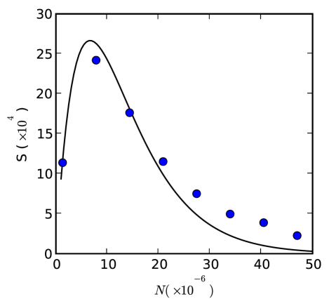
Figure 5: (color online) The maximum value of the interference signal as a function of number of atoms in the trap. The solid curve is Eq. (38) and the dots were extracted from a DSMC calculation.

Figure 5 shows the maximum value of the interference as a function of number of trapped atoms $N$. The solid curve was found using Eq. (38) and the dots were extracted from our DSMC code. The remaining parameters are the same as in Fig. 2. When the number of atoms in the gas is $N<7\times 10^{6}$, the signal increases with increasing number. This is because as the number of atoms increases so does the amount of back scattered light. When the total number of atoms in the gas is $N>7\times 10^{6}$ the interference signal decreases because the higher density increases the collision rate between the atoms in the gas. Using Eq. (38) it can be shown that, holding all other parameters constant, the maximum value of the interference signal occurs the number of atoms is

$$N=\frac{2^{1/2}\pi T}{n\omega_{\perp}^{2}\sigma}.$$ (41)

For a trap with frequencies $\omega_{\parallel}=2\pi\times 3\mbox{Hz}$ and $\omega_{\perp}=2\pi\times 300\mbox{Hz}$, that traps ${}^{87}\mbox{Rb}$ atoms at $40~{}\mu\mbox{K}$ the optimal number of atoms for one trap period is about $7\times 10^{6}\mbox{atoms}$. To measure Earth’s rotation with at $\pi$ phase shift, by displacing the trap by $5~{}\mbox{mm}$, the atoms must oscillate three time in this trap and the optimal number of atoms is $2.2\times 10^{6}$.

IV Conclusions

In this paper we presented a simple analytic model of the dynamics of a trapped atom interferometer that uses a single Kapitza-Dirac pulse to modulate the atoms and the classical turning points of the trap to reflect them. The interferometers signal is read out by reflecting a single probe pulse off of the atoms and interfering the back-reflected light with a reference beam. We presented a description of the collisions between the atoms and showed that our simple model give quantitatively accurate results when compared to a DSMC model of the interferometer. Finally, we used our model to find the optimal temperature or number to maximize the performance of the interferometer.

Although the analytic model presented in this paper specialized to the analysis of a single Kapitza-Dirac pulse, the results of Sec. III easily generalize to multi-pulse interferometers Wu et al. (2007b); Su et al. (2008). To apply our model to interferometers that use gases above the BEC transition temperature but below the recoil temperature the momentum and spacial dependence on the collision frequency cannot be ignored and Eq. (12) must be used instead of Eq. (16). We believe that inclusion of the more complicated collision frequency will not dramatically change the results of this paper when describing a gas below the recoil temperature.

V Acknowledgements

We would like to thank Alexey Tonyushkin, Mara Prentiss, Alex Zozulya, and Val Bykovsky for their useful conversations on this subject. The authors acknowledge support from the Air Force Office of Scientific Research under program/task 2301DS/03VS02COR and DARPA.

References

- Durfee et al. (2006) D. S. Durfee, Y. K. Shaham, and M. A. Kasevich, Phys. Rev. Lett. 97, 240801 (2006).
- Hogan et al. (2008) J. M. Hogan, D. M. S. Johnson, and M. A. Kasevich, arXiv:0806.3261v1 (2008).
- Peters et al. (1999) A. Peters, K. Y. Chung, and S. Chu, Nature 400, 849 (1999).
- Schumm et al. (2005) T. Schumm, S. Hofferberth, L. M. Andersson, S. Wildermuth, S. Groth, I. Bar-Joseph, J. Schmiedmayer, and P. Kruger, Nature Phys. 1, 57 (2005).
- Wang et al. (2005) Y.-J. Wang, D. Z. Anderson, V. M. Bright, E. A. Cornell, Q. Diot, T. Kishimoto, M. Prentiss, R. A. Saravanan, S. R. Segal, and S. Wu, Phys. Rev. Lett. 94, 090405 (2005).
- Garcia et al. (2006) O. Garcia, B. Deissler, K. J. Hughes, J. M. Reeves, and C. A. Sackett, Phys. Rev. A. 74, 031601(R) (2006).
- Horikoshi and Nakagawa (2006) M. Horikoshi and K. Nakagawa, Phys. Rev. A. 74, 031602(R) (2006).
- Jo et al. (2007) G.-B. Jo, Y. Shin, S. Will, T. A. Pasquini, M. Saba, W. Ketterle, D. E. Pritchard, M. Vengalattore, and M. Prentiss, Phys. Rev. Lett. 98, 030407 (2007).
- Wu et al. (2007a) S. Wu, E. Su, and M. Prentiss, Phys. Rev. Lett. 99, 173201 (2007a).
- Deissler et al. (2008) B. Deissler, K. J. Hughes, J. H. T. Burke, and C. A. Sackett, Phys. Rev. A. 77, 031604(R) (2008).
- Javanainen and Wilkens (1997) J. Javanainen and M. Wilkens, Phys. Rev. Lett. 78, 4675 (1997).
- Leggett and Sols (1998) A. J. Leggett and F. Sols, Phys. Rev. Lett. 81, 1344 (1998).
- Javanainen and Wilkens (1998) J. Javanainen and M. Wilkens, Phys. Rev. Lett. 81, 1345 (1998).
- Cronin et al. (2007) A. D. Cronin, J. Schmiedmayer, and D. E. Pritchard, arXiv:0712.3703v1 (2007).
- Cahn et al. (1997) S. B. Cahn, A. Kumarakrishnan, U. Shim, T. Sleator, P. R. Berman, and B. Dubetsky, Phys. Rev. Lett. 79, 784 (1997).
- Horikoshi and Nakagawa (2007) M. Horikoshi and K. Nakagawa, Phys. Rev. Lett. 99, 180401 (2007).
- Wu et al. (2007b) S. Wu, P. S. Striehl, and M. G. Prentiss, arXiv:0710.5479v2 (2007b).
- Burke et al. (2008) J. H. T. Burke, B. Deissler, K. J. Hughes, and C. A. Sackett, Phys. Rev. A. 78, 023619 (2008).
- Stickney et al. (2008) J. A. Stickney, R. P. Kafle, D. Z. Anderson, and A. A. Zozulya, Phys. Rev. A. 77, 043604 (2008).
- Su et al. (2008) E. J. Su, S. Wu, and M. G. Prentiss, arXiv:physics/0701018v2 (2008).
- Stickney et al. (2007) J. A. Stickney, D. Z. Anderson, and A. A. Zozulya, Phys. Rev. A. 75, 063603 (2007).
- Akhiezer and Peletminskii (1981) A. Akhiezer and S. Peletminskii, Methods of Staistical Physics (Pergamon Press, Oxford, 1981).
- Chpman and Cowling (1970) S. Chpman and T. Cowling, The Mathematical Theory of Non-Uniform Gases (Cambridge at the University Press, Cambridge, 1970), 3rd ed.
- Garcia (2000) A. L. Garcia, Numerical Methods for Physicis (Prentice Hall, New Jersey, 2000), 2nd ed.