Stabilization of vortex-antivortex configurations in mesoscopic
superconductors by engineered pinning

Abstract

Symmetry-induced vortex-antivortex configurations in superconducting squares and triangles were predicted earlier; yet, they have not been resolved in experiment up to date. Namely, with vortex-antivortex states being highly unstable with respect to defects and temperature fluctuations, it is very unlikely that samples can be fabricated with the needed quality. Here we show how these drawbacks can be overcome by strategically placed nanoholes in the sample. As a result, (i) the actual shape of the sample becomes far less important, (ii) the stability of the vortex-antivortex configurations in general is substantially enhanced, and (iii) states comprising novel giant-antivortices (with higher winding numbers) become energetically favorable in perforated disks. In the analysis, we stress the potent of strong screening to destabilize the vortex-antivortex states. In turn, the screening-symmetry competition favors stabilization of new asymmetric ground states, which arise for small values of the effective Ginzburg-Landau parameter $\kappa^{*}$.

I Introduction

The question of vortex-antivortex (VAV) states in mesoscopic samples is one of the most intriguing ones in superconductivity studies of the last decade. Being stabilized in a homogeneous magnetic field, VAV states are counterintuitive and rather difficult to explain in usual terms. Nevertheless, by analyzing the solutions of the linearized Ginzburg-Landau (GL) theory, Chibotaru et al. VAVNature predicted their stability in flat superconducting squares as a consequence of the symmetry of the sample. Namely, in linear theory, the geometry of the sample boundaries directly translates on the vortex states. As a consequence, for three fluxons captured by the sample (i.e. vorticity $L=3$), the vortex state with four vortices and one antivortex can be energetically more favorable than the triangular configuration of single vortices. Still, one should bear in mind that the linear approach of Ref. VAVNature is only valid at the superconducting/normal (S/N) boundary, where $\Psi$ is extremely small and the non-linear term in the GL theory becomes negligible. In a further step VAVJahnTeller ; VAVStability , by taking into account the non-linearity of the first GL equation, the existence of VAV states was predicted to persist even away from the S/N phase boundary. The antivortex for $L=3$ in a square of size $10\xi_{0}\times 10\xi_{0}$ was shown to be stable in a temperature range of about $\Delta T=0.3T_{c}$ (with $\xi_{0}$ being the coherence length at $T=0$, and $T_{c}$ the critical temperature). Up to now, such VAV configurations have not been realized in experiment. From a theoretical viewpoint, there are several reasons why these novel vortex states escaped experimental observation: first, even a tiny defect at the boundary ($<1\%$) destroys the vortex-antivortex state VAVEdgeDefect . Second, the vortices and the antivortex are all confined in a small area of typical size less than the coherence length $\xi(T)$. As a consequence, this proximity results in a strong local suppression of the order parameter $\Psi$ which makes the separate minima experimentally undistinguishable - the vortex configuration as a whole is very similar to a single giant-vortex. And third, imaging of the magnetic field profile is also shortcoming: the field generated by the sample is proportional to the supercurrent which is rather weak in the VAV region (being directly related to $\Psi$).

Therefore, for future experimental verification of the VAV states, it is essential: i) to increase the vortex-antivortex distance, allowing for measurements with realistic spatial resolution; ii) to obtain a larger contrast in the order parameter, and iii) the magnetic field, required for e.g. Scanning Tunnelling and Hall-probe microscopy measurements. However, to observe the ’pure’ VAV nucleation, we should realize this in a homogeneous magnetic field, contrary to the suggestion of Ref. VAVMagneticDot where a magnetic dot was placed on top of the sample. It is already well-known that VAV states have low energy in an inhomogeneous magnetic field, such as the stray field of the magnetic dots MiloPRL which may induce antivortices in its own.

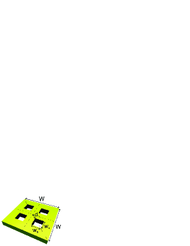
Figure 1: (Color online) Superconducting square with four nanoholes (i.e. antidots).

In our recent Letter MyPRL , we introduced the idea of strategically made perforations/holes/antidots in a square mesoscopic superconductor (see Fig. 1) which act as pinning centers for the vortices. The pinning force is supposed to pull the vortices further from the sample center and thus create a larger separation between the vortices and the central antivortex. In what follows, we will elaborate further on this concept, and demonstrate a number of its advantages. Contrary to Ref. MyPRL where we considered only the square geometry, here we expand the study to different polygonal shapes of the sample and geometry of the pinning. In addition, while previous studies VAVNature ; VAVTriangleLGL ; VAV2 ; VAVJahnTeller only studied VAV configurations in extremely thin samples, we consider samples of finite (though relatively small) thickness, by incorporating magnetic screening effects in the calculation.

The paper is organized as follows. First the theoretical approach is formulated (Sec. II), comprising the full non-linear GL theory and the linearized GL theory (LGL). In Sec. III we present our results, and determine the optimal pinning parameters to enhance the stability range of the vortex-antivortex configuration. The influence of imperfections and defects on the superconducting state is discussed in Sec. IV, the competition of different symmetries in the sample is treated (Sec. V), e.g. a disk with a number of holes. Next we describe the influence of the non-linear term in GL theory and GL parameter $\kappa$, i.e. screening (Sec. VI) and some guidelines for a possible experimental observation (Sec. VII). Finally, we summarize our findings in Sec. VIII.

II Theoretical formalism

II.1 Ginzburg-Landau theory

It is already well established that the Ginzburg-Landau (GL) formalism gives an accurate description of the superconducting state of low-$T_{c}$ superconductors, and is well suited to incorporate boundary effects in the treatment of the mesoscopic superconductors. The GL theory postulates the following expression for the free energy of the system (in dimensionless form):

$$\mathcal{F}=\int{\bf dr}\left[-2|\Psi|^{2}+|\Psi|^{4}+2\left|\left(-i{\bf\nabla}-{\bf A}\right)\Psi\right|^{2}\right.$$

$$\left.+2\kappa^{2}\left({\bf B}-{\bf B}_{appl}\right)^{2}\right].$$ (1)

Here all distances are measured in units of the coherence length $\xi(T)=\xi_{0}/\sqrt{1-T/T_{c}}$. The vector potential ${\bf A}$ is expressed in units of $c\hbar/2e\xi$, the magnetic field in units of $H_{c2}=\hbar/2e\xi^{2}$, and the complex order parameter $\Psi$ in units of $\Psi_{0}=\sqrt{-\alpha/\beta}$, such that $|\Psi|=1$ in the pure Meissner phase and $|\psi|=0$ in the normal conducting state (with $\alpha,\beta$ being the GL coefficients Tinkham ). $|\Psi|^{2}$ represents the local Cooper-pair density, which we will abbreviate as CPD. ${\bf B}_{appl}$ denotes the applied magnetic field, while ${\bf B}$ stands for the total magnetic field. $\kappa$ is the ratio between penetration depth and coherence length, i.e. $\kappa=\lambda/\xi$ and is assumed temperature independent in this model

To find stable solutions, one has to find the wave function and the vector potential which minimize the free energy functional. Two coupled non-linear differential equations, one for the order parameter and one for the vector potential, can be derived using variation analysis. We are interested in thin, but finite-thickness, samples in a perpendicular applied field, where we may neglect the variation of the magnetic field and order parameter over the thickness of the sample. Accordingly, we average the GL equations over the sample thickness schw ; Tinkham ; Prozorov , and write them as

$$\left(-i{\bf\nabla}-{\bf A}\right)^{2}\Psi=\Psi\left(1-|\Psi|^{2}\right),$$ (2)

$$-\kappa^{*}\Delta{\bf A}={\bf j}_{s}=\Re\left(\Psi^{*}(-i{\bf\nabla}-{\bf A})\Psi\right),$$ (3)

where ${\bf j}_{s}$ denotes the supercurrent density, and $\kappa^{*}=\kappa^{2}/(d/\xi)$ is the effective Ginzburg-Landau parameter, the consequence of averaging over sample thickness $d$. It’s worth emphasizing that $\kappa^{*}$ is temperature dependent (e.g. through $\xi(T)$ in the denominator). All considered samples in this paper, treated with the full non-linear GL theory, have the same thickness $d=\xi_{0}$. Consequently $\kappa^{*}$ takes the temperature dependence $\kappa^{*}(T)=\kappa^{2}/\sqrt{1-T}$. To address properly the influence of $T$, all results obtained by the full GL theory will be expressed in units of $\xi$, $\psi_{0}$ and $H_{c2}$ at zero temperature.

While authors of Refs. VAVNature ; VAVTriangleLGL ; VAV2 ; VAVJahnTeller solved only the first GL equation, and restricted themselves to the limit of $d\rightarrow 0$, or extreme type II superconductors, we solve numerically both equations. The strength of the influence of the second GL equation is governed by $\kappa^{*}$. When $\kappa^{*}\gg 1$ (thus for $d\ll 1$ and/or $\kappa\gg 1$), Eq. (3) can indeed be neglected. However, when $\kappa^{*}\approx 1$, we found it can have a tremendous influence and provide us with some interesting and novel behavior of the superconducting state.

After solving Eqs. (2-3), the vorticity $L$ of the found stable vortex configuration is defined as the sum of the individual winding numbers of all vortices present in the sample. The winding number of a vortex is defined as the integer number of $2\pi$ phase changes of the order parameter when circling around the vortex core. Consequently, the vorticity of a vortex is defined as 1, and the vorticity of an antivortex as -1. The total vorticity of a particular vortex configuration can also be determined at the sample boundary $\Omega$ by the formula

$$L=-\frac{1}{2\pi}\oint_{\Omega}i\ln(\psi/|\psi|).$$ (4)

The vortex state of small mesoscopic superconductors is strongly influenced by the imposed topological confinement. The shape of the sample boundaries is introduced in our calculation through the Neumann boundary condition, which sets the supercurrent perpendicular to the boundary equal to zero:

$${\bf n}\cdot\left.\left(-i{\bf\nabla}-{\bf A}\right)\right|_{\text{boundary}}=0,$$ (5)

where ${\bf n}$ is the normal unit vector on the surface. In Refs. VAVNature ; VAVTriangleLGL ; LeuvenGauge a unitary transformation was used in combination with a certain gauge for the vector potential such that for the linear GL equation ${\bf A}=0$ on the sample boundary. This approach is restricted to simple geometries (i.e. polygons) and cannot be applied to our multiple connected samples that contain holes.

Our numerical approach is based on a finite difference Gauss-Seidel relaxation for the time dependent GL equations. The numerical technique we applied is the one introduced in Ref. Kato with convenient iterative expansion of the non-linear term explained in Ref. schw , to speed up convergence. We solve the GL equations on a uniform Cartesian grid typically with $128\times 128$ points.

II.2 Linearized approach

Since the VAV state is a consequence of the symmetry of the sample boundary and because of the most efficient reflection of this symmetry into the solutions of the linearized Ginzburg-Landau (LGL) theory, the LGL formalism is the ideal instrument to study the influence of the geometry on the VAV state. From a numerical point of view, the LGL approach is far less demanding, and can still provide us with the minimal requirements for the realization of the VAV states.

The linear theory is exactly valid only on the S/N boundary, i.e. when the $|\Psi|^{3}$ term can be neglected. Due to the weak superconducting order parameter, the magnetic field equals the applied one and the second GL equation can be discarded. At the same time, Eq. (2) becomes

$$(i{\bf\nabla}+{\bf A})^{2}\psi=\alpha\psi,$$ (6)

where $\alpha$ now is equivalent to an eigenvalue. An important property of Eq. (6) is that its solution is independent of the size of the sample, as long as the applied flux is held constant, i.e. the LGL method is a scalable theory.

To be able to compare the solutions of the LGL obtained for different geometries, one has to make sure that they have the same normalization. We use the following normalization of the wave function, $\frac{1}{V}\int_{V}dV|\Psi|^{2}$ = 1, or equivalently $\langle|\Psi|^{2}\rangle=1$, where the integration is performed over the sample volume $V$. This matches the uniform solution of $|\Psi|=1$ in the whole sample in the absence of a magnetic field.

Our aim is to use the LGL model deeper inside the superconducting state, even though it is strictly not valid, simply as a limiting case of the full GL theory. For that purpose we still derive the generated magnetic field profile using Eq. (3). Although the LGL theory is not able to determine an absolute order of magnitude of the field (because $\Psi\approx 0$), it gives the correct magnetic field up to a multiplication constant, and thus allows for comparison of field profiles for different sample geometries.

We compute the vector potential ${\bf A}$ from the calculated distribution of supercurrents, for taken $\kappa^{*}=1$. For this purpose, we solve two independent Poisson equations (for $A_{x}$ and $A_{y}$) using the Fast Fourier Transform. Magnetic field is then obtained as ${\bf B}={\bf\nabla}\times{\bf A}$. The relative magnetic field profile found in this way turns out to be rather accurate, even when going deeper in the superconducting state (e.g. by decreasing temperature). When compared with a calculation based on the full non-linear GL theory, the main effect of the second equation is to enhance the magnetic field generated by the sample.

As an advantage, to solve Eq. (6) is computationally not very demanding, and we use the numerical package COMSOL (formerly known as Femlab) for this purpose. This software package uses the finite element method to solve differential equations. Its profound precision (in solving linear equations) allows us to significantly increase the grid resolution, for instance, in the neighborhood of the VAV complex. The use of triangular finite elements proved as a more accurate treatment of the sample’s geometry than we could achieve with a rectangular grid, for an arbitrary sample geometry.

Therefore, our linear approach is well suited for comparison of the VAV state in different samples. We will use it to determine the optimal hole parameters and to study the influence of imperfections and defects. We will also treat the competition of different pinning symmetries and samples with different geometries, like e.g. perforated disks, in search for novel VAV states.

III Engineering of the artificial pinning sites

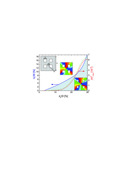
Figure 2: (Color online) Blue solid curve: The minimum size $W_{h}$ of the hole for the vortices to be fully captured by the holes at distance $d_{h}$. Above the blue line, vortices are contained in the holes. Below the blue line, vortices are outside and between the holes. Red dashed curve: The maximum CPD between the vortex and the antivortex when the holes are minimum sized. Green dotted curve: Dimensionless quantity $\Delta B_{vav}$, expressing the strength of the magnetic field difference measured in the vortex and in the antivortex. Insets are contour plots of the phase of the wave function (blue/red corresponds to 0/2$\pi$) for $d_{h}/D=28\%$ and $w_{h}/W=18\%$ (upper) and $d_{h}/D=36\%$ and $w_{h}/W=14\%$ (lower). The applied flux $\phi=5.5\phi_{0}.$

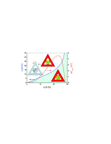
Figure 3: (Color online) Blue solid curve: The minimum size $W_{h}$ of the hole for the vortices to be fully captured by the holes at distance $d_{h}$. Above the blue line, vortices are contained in the holes. Below the blue line, vortices are outside and between the holes. Red dashed curve: The maximum CPD between the vortex and the anti vortex when the holes are minimum sized. Green dotted curve: Dimensionless quantity $\Delta B_{vav}$, expressing the strength of the magnetic field difference measured in the vortex and in the antivortex. Insets are contour plots of the CPD of the wave function (blue/red corresponds to low/high density - logarithmic color scale) for $d_{h}/D=22\%$ and $w_{h}/W=24\%$ (upper) and $d_{h}/D=24\%$ and $w_{h}/W=18\%$ (lower). The applied flux $\phi=3.5\phi_{0}.$

In what follows, we will study the optimal parameters of the artificial pinning centra, i.e. size and position of the holes introduced in the mesoscopic sample, using the linear GL theory. Later on, the influence of the non-linearity of the GL equations and the inclusion of the second GL equation will be systematically investigated.

Our aim is to enhance the parameters that characterize the VAV state. These are: (i) the maximal Cooper-pair density (CPD) between the V and AV ($|\psi|_{max}^{2}$) because of the need of CPD imaging techniques (e.g. STM) for a sufficient contrast in the local density of states, (ii) the distance between V and AV ($d_{vav}$) which has to be larger than the spatial resolution of the measurements, and (iii) the magnetic field difference between V and AV ($\Delta B_{vav}$). All the latter properties for a given VAV state are defined for the VAV pair with smallest separation $d_{vav}$.

The influence of the holes on the vortices is determined by their position and their size. How can we enhance e.g. the vortex-antivortex separation by manipulating these parameters? Holes are known to be pinning sites, i.e. they attract vortices. By placing four holes, we can pull the vortices, which surround the antivortex, away from the antivortex. The larger the hole, the stronger the attraction. The forces on the antivortex are exactly cancelled because of the symmetric position of the holes. However, the vortices also experience inward forces, i.e. they are attracted by the antivortex and additionally the Meissner current also compresses the vortices to the inside of the sample. The vortices eventually will find an equilibrium position, in which the inward and outward forces cancel exactly. This position depends of the distance of the hole to the center and of the size of this hole.

To understand the influence of the hole parameters (size and position) we introduce a criterium which we can use as a guide to determine the optimal hole parameters. This criterium is: What is the minimum hole size for a given hole position, such that the vortex is still captured by the hole? It seems that when holes are made larger, they attract the vortices more strongly and eventually the vortex will be captured by the hole, when the holes are placed not too close to the boundary of the sample. We show our results in Fig. 2 and Fig. 3 for the square and the triangle geometry, respectively. The insets show the setup and the definition of the hole parameters. The characteristic variables $d_{h}$($=d_{vav}$), $|\psi|_{max}^{2}$ and $\Delta B_{vav}$ are also shown in Figs. 2 and 3.

We note that the curves of $|\psi|_{max}^{2}$ and $\Delta B_{vav}$ are isomorphous. We expect this, because $|\psi|_{max}^{2}\propto|\psi|^{2}\propto j_{s}\propto\Delta B\propto\Delta B_{vav}$. The maximum $|\psi|_{max}^{2}$ and, as a consequence, $\Delta B_{vav}$ in a triangle appear to be 40 % less than for the square.

From these figures, we can conclude that, for both the square and the triangle shaped samples, moving the holes farther from the center implies enlarging them, in order to keep the vortices trapped by the holes. From a certain distance $d_{h}$, the needed hole size $w_{h}$ diverges, i.e. from a certain distance of the holes, they can never be made large enough to trap the vortices that surround the antivortex. For both the square and the triangle, this distance $d_{h}/D$ is about 30%. While for the square increasing the distance always implies an increase of $|\psi|_{max}^{2}$ and $\Delta B_{vav}$, this is not true for the triangle: from a distance $d_{h}/D\approx 23\%$ these observables start degrading.

However these results apply to a specific shape of the holes, and in principle it is not fair to compare the perforated square with the perforated triangle, since the holes have different shape. For the square, the trapped vortex is located in the corner of the square hole; for the triangle this vortex is located in the middle of a side. Thus, as an alternative approach we reinvestigated both samples, now with circular holes, and noticed that qualitatively these results do not differ from the ones with the other shaped holes. Consequently, we conclude that the general conclusions for square and triangle are independent of the shape of the holes.

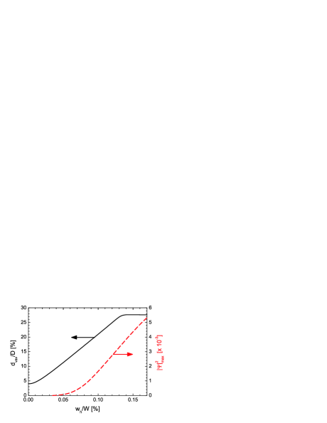
Figure 4: (Color online) VAV distance ($d_{vav}$) and the maximal value of the CPD between the VAV ($|\psi|^{2}_{max}$) versus the hole size $w_{h}$ for a square with square holes at position $d_{h}/D=28\%$. Applied flux $\phi=5\phi_{0}$.

When, in a realistic situation, one is interested in capturing the vortices by the holes, one has to chose a somewhat bigger hole size than the minimal one since small defects will distort the VAV state and drive a VAV pair closer to each other, hereby the vortex leaving the hole.

For holes at a distance of $d_{h}/D=28\%$, the influence of the hole size is depicted in Fig. 4. However a larger hole size will of course not increase the VAV distance, it will increase $|\psi|_{max}^{2}$ which is important for the needed experimental resolution.

IV Influence of imperfections/defects

By introducing nano-engineered holes, we enhanced the observability of the VAV state. But how about its stability against defects?

It is generally known that the VAV state in a plain square is very vulnerable to defects positioned at the edge of the sample VAVEdgeDefect . We will show how this situation dramatically changes when fourfold symmetric holes are introduced into the sample. We will consider defects as slight modifications of the geometry using the linear GL theory. We observe that when the linear theory predicts that the vortex-antivortex pair annihilates, it will surely be so in the non-linear theory, which justifies the use of the LGL theory, in order to determine the minimal requirements for the stability of the VAV state.

IV.1 A defect at the edge

As a starting point for comparing the perforated sample with the plain sample we will study the influence of defects at the edge of the sample. It is generally known that a small defect at the boundary will destroy the VAV state in a plain square VAVEdgeDefect . In the present study we restrict ourselves to defects that are indentations and bulges at the surface of the sample. We will present here the results for a square for two different defects positioned at the edge of the sample. The defect under study is placed at the center of the edge of the square and is taken to be a square itself with side $w_{d}$. We considered a small bulge and a small indentation. It is known that such defects may influence the penetration and expulsion of vortices as was demonstrated experimentally by A. K. Geim et. al in Ref. geim . For theoretical studies we refer to Refs. peetersdefect and baelusdefect .

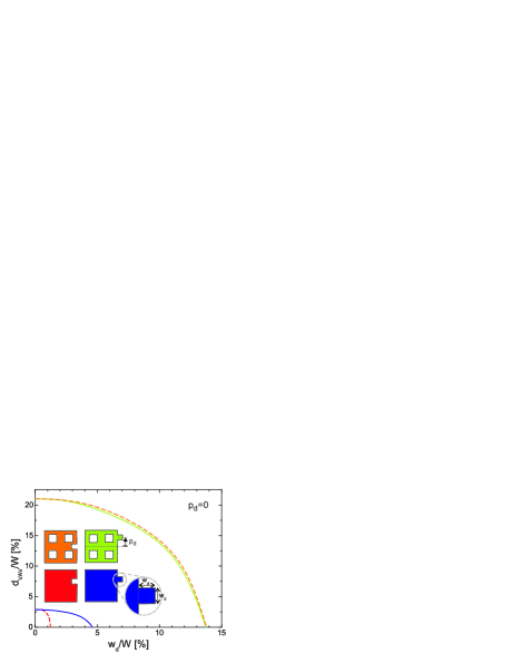
Figure 5: (Color online) The vortex-antivortex distance vs defect size for a plain (dark grey) and a perforated (light grey) square, with a square defect at the middle of one edge, i.e. $p_{d}=0$. The dashed curve represents an indentation, the solid curve a bulge defect. The applied flux for the plain square $\phi=5.5\phi_{0}$ and for the perforated square $\phi=4.0\phi_{0}$

We focus on the VAV separation $d_{vav}$ to compare the influence of defect size between the perforated square and the plain square. When this distance equals zero, the VAV pair annihilates and the VAV configuration disappears. The results for the plain square are shown by the two curves at the lower left region of Fig. 5. The results for the perforated square are shown by the two curves at the upper right region. The hole size and position used for the perforated square are $W_{h}/W=20\%$ and $d_{h}/D=28\%$. For the plain square we applied a flux $\phi=5.5\phi_{0}$, for the perforated square $\phi=4.0\phi_{0}$. We had to apply different fluxes since the stability range of the L=3 state in both samples do not overlap. (The introduction of holes shifts the phase diagrams to lower flux.)

For a plain square with a bulge defect, we conclude that the VAV configuration exists until a size $w_{d}/W\sim 5\%$. The VAV state is even more sensitive to an indentation: a size of $\sim 1\%$ is sufficient for the disappearance of the VAV. However, we found that the perforated square is much more resistant to defects. Bulge and indentation defects, up to 14% (comparable to the size of a nano-hole), now coexist with a VAV configuration. Bulge and indentation defects have a similar effect on the VAV stability, in contrast to the plain square case. We conclude that the 4-fold symmetrically placed pinning centers are much more efficient in imposing their symmetry than the outer boundary of the sample. As a consequence, small defects at the edge have little effect and only distort the VAV molecule

One may argue that this effect is possibly only since the defect is located exactly in the center of the edge, therefore imposing mirror symmetry. Because of this symmetry, the antivortex is prohibited to chose one of the two vortices of the holes to annihilate with and it stays on the mirror line.

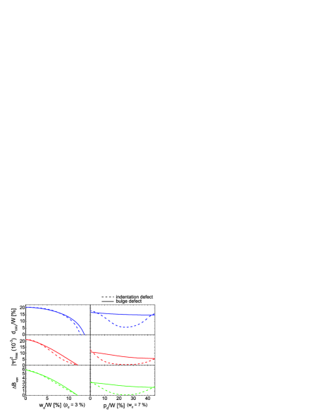
Figure 6: (Color online) The influence of a defect on the vav distance ($d_{vav}$), CPD between vortex and antivortex ($|\psi|_{max}^{2}$) and the magnetic field difference between vortex and antivortex ($\Delta B_{vav}$). The hole parameters are $w_{h}/W=20\%$ and $d_{h}/D=28\%$ and the applied flux $\phi=4\phi_{0}.$.

To turn off this stabilization effect due to symmetry, we also investigated defects which are displaced from the middle of the edge. We studied the influence of the position and size of an edge defect on the characteristic parameters $d_{vav}$, $|\psi|_{max}^{2}$ and $\Delta B_{vav}$. The result is shown in Fig. 6 for a perforated square with hole parameters $w_{h}/W=20\%$ and $d_{h}/D=28\%$ under an applied flux of $4\phi_{0}$. On the left side, the influence of the defect size is depicted for both a bulge and an indentation defect, positioned at a distance $p_{d}/W=3\%$ from the edge center. On the right side, the influence of the position of a defect of size $w_{d}/W=7\%$ is shown.

Concerning the influence of the size of the defect, we notice that bulge and indentation defect act similarly: Increase of the defect size implies degradation of all three observables $|\psi|_{max}^{2}$, $d_{vav}$ and $\Delta B_{vav}$. However, for the position of the defect, we predict different behavior for bulge and indentation. For a bulge defect, we notice that the stability of the VAV configuration decreases as the defect moves further from the center of a side, while for the indentation we observe a decrease followed by an increase. However, for both types of defects, the VAV configuration survives best when the defect is centered at an edge. We also conclude that a bulge defect is less destructive than an indentation, unless it is placed near the center of an edge. The antivortex acts like being attracted to the indentation and repelled by the bulge defect.

IV.2 Other kinds of defects

The VAV stability against edge defects is strongly improved by the introduction of the fourfold symmetrically placed holes. However, in actual experiments these holes themselves can contain defects or imperfections such as non-uniform sized holes, holes which are a little displaced with respect to their high symmetry position, or holes with a slightly different shape.

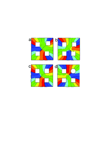
Figure 7: (Color online) Contourplots of the phase of the order parameter in a perforated square with several kinds of defects. The hole parameters are: $w_{h}/W=20\%$, $d_{h}/D=22\%$ and applied flux $\phi=4.1\phi_{0}$. The defects include: a) a diagonally displaced hole, b) a horizontally displaced hole, c) a bigger hole and d) a different shaped hole.

In Fig. 7 four examples are shown. In all pictures the ‘normal’ holes can be described by the parameters $w_{h}/W=20\%$, $d_{h}/D=22\%$ and we apply a magnetic flux $\phi=4.1\phi_{0}$. The plots in Figs. 7 (a) and (b) illustrate the effect of imperfect positioned holes. In Fig. 7 (a), a diagonal displacement of the upper right hole over a distance $d/W=6\%$ is shown. The VAV survives such displacements in the range of -4% to +12%. For a horizontal displacement, as illustrated in b), the range is smaller: from -3.5% to +3.5%. The fact that the VAV configuration is more stable for a diagonal displacement, we attribute to the existence of mirror symmetry along one diagonal, forcing the AV on this diagonal.

In Fig.7 (c) the upper right hole has a somewhat larger size than the other holes. Its sides are $5\%$ larger. This kind of hole size defect does not destroy the VAV state, when in the range of -8% to +9%.

In Fig. 7 (d) the upper right hole is circular. It has the same area as the square holes and is centered like the square holes. The VAV survives, which illustrates that it’s not the exact shape of the holes which matters, but rather its area. This implies that non perfect holes, i.e. holes with defects, will not destroy the VAV state as long as the imperfection is not too large.

V Competing symmetries

V.1 Superconducting samples with polygonal pinning

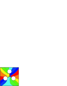
Figure 8: (Color online) Contourplot of the phase of the order parameter for a square sample with three circular holes. The state with vorticity 2 is shown. The symmetric positioning of the holes induces an antivortex in the center.

Several symmetries compete with each other when the VAV state nucleates. First we have the vortex-vortex interaction through which the vortices will try to form the Abrikosov triangle lattice. Second there is the sample boundary which will impose its own symmetry, and third there are the pinning centers (i.e. the holes) which will also try to impose their own symmetry.

For small samples of the order of several coherence lengths, like the ones we studied up to now, the symmetry of the sample boundary opposes the Abrokisov lattice. In this subsection we’ll point out that the symmetry of the pinning sites is even more strongly dominating than the symmetry of the boundary.

For example we show the VAV state with vorticity $L=3-1=2$ in a square with three holes in Fig. 8. Although the outer edge has a square geometry it is the triangular arrangement of the circular holes which imposes its symmetry on the superconducting wave function in the center of the square. This leads to 3 vortices trapped in the holes and a single antivortex in the middle of the sample.

V.2 Superconducting disk with many holes

The arrangement of holes, instead of the sample outer boundary, seems to be the geometry element which is much more effective in imposing its geometry on the wave function. For this reason, we can as well use circular symmetric disks, perforated by N symmetrically placed holes, and expect an N-fold symmetric CPD. A large variety of symmetry induced antivortex configurations can be created this way. Following this approach we found that it was possible to even create giant anti-vortices with vorticity $L$ up to $-7$.

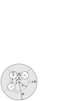
Figure 9: The parameters $R$, $\rho$, $r$, $d$ and $\theta$, used to characterize the geometry of the disk with N holes.

The parameters which define the geometry are depicted in Fig. 9. $d$ is the distance between holes, $\theta$ the angle between holes which is set equal to $2\pi/N$, as to impose the N-fold symmetry. There is also $\rho$, the distance of the holes’ center to the disks center. $R$ is the radius of the disk and $r$ is the radius of the holes. Imposing that the distance between the holes equals the hole’s diameter is equivalent to the condition $r=(1/2)\rho\sin(\theta/2)$.

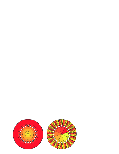
Figure 10: (Color online) Disk with 20 holes, in the state with vorticity L=19, consisting of 20 vortices and 1 antivortex in the center. Left: Logarithm of CPD Contour plot (Red (Dark grey)/Yellow (Light grey) = High/Low density) Right: Phase Contour plot (Red (Dark grey)/Yellow (Light grey)= 0/2$\pi$)

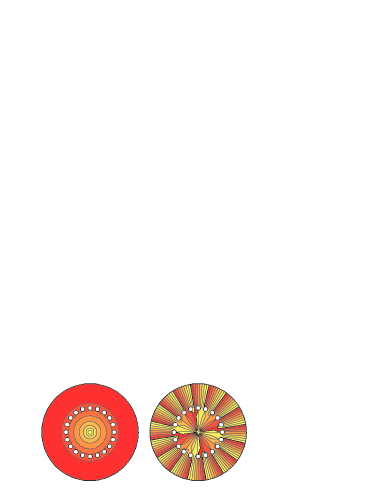
Figure 11: (Color online) Disk with 20 holes, showing 4 antivortices in the center. Left: Logarithm of CPD Contour plot (Red (Dark grey)/Yellow (Light grey) = High/Low density) Right: Phase Contour plot (Red (Dark grey)/Yellow (Light grey)= 0/2$\pi$)

To illustrate this conjecture, we give some examples. In Fig. 10 the CPD and the phase plot of a disk with 20 holes is shown. The parameters are $r/R=4.3\%$, $\rho/R=55\%$, so that the distance between the holes $d=2r$. The applied flux is $\phi=26\phi_{0}$. The vorticity $L=19$, is one less the symmetry of the holes and consequently an additional vortex-antivortex pair is created. The alternative solution to obey the symmetry would be to create a $L=19$ giant vortex, but it turns out that the creation of one VAV pair is energetically more favorable.

There’s clearly a competition between the formation of a giant vortex - the merging of several vortices in one point - and the formation of a giant antivortex - consisting of the creation of vortex-antivortex pairs and then merging of all anti-vortices in a singular point.

For the same disk, with an applied flux of $\phi=21\phi_{0}$ and slightly modified parameters $\rho/R=0.5$ and $r/R=4.73\%$ the CPD and the corresponding phase plot is shown in Fig. 11. The phase plot indicates a giant antivortex in the center with winding number -4. We found that the giant antivortex is highly unstable with respect to defects. Therefore, in experiment, it will be very difficult, to observe these giant antivortices, and most likely they will fall apart in 4 single antivortices. The reasons for this are: i) a sample with a perfect symmetry and in the absence of defects will be difficult to manufacture. In a first stadium, the imperfections will cause the giant AV to disassociate into separate antivortices and for larger imperfections it will cause the VAV pairs to annihilate. ii) The extreme low CPD in the center due to the densely packed (anti-)vortices which is almost impossible to distinguish between the separate minima.

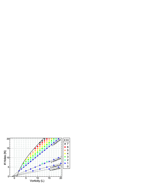
Figure 12: (Color online) For each vorticity and for each number of holes N, the number of anti-vortices is shown. Due to the symmetry the antivortices combine to a giant antivortex. Left of the thick line no antivortices are observed.

To generalize the concept of giant-antivortices and their appearance in disks with N symmetrically placed holes, we investigated the relation between the symmetry order N and the vorticity L. The result is the L-N phase diagram shown in Fig. 12 where we used the following parameters: $\rho/R=0.55$, $r=2d$ and $\phi=1.2N\phi_{0}$.

The anti-vorticity of the state is indicated by the different colors. When $L<N$, and there are no anti-vortices, a giant vortex of vorticity L is located at the disk center, since this is the only solution which is able to obey the symmetry. However, because of the finite grid resolution, these vortices split up in separate ones, analogous to the fate of the giant antivortex described before.

For vorticities $L\geq nN$ (where $n$ is the largest integer obeying the condition) another property is observed: every hole pins $n$ vortices, which are not necessarily captured inside the holes, but clearly belong (i.e. are attached) to the specific hole.

The L-N phase diagram is not uniquely determined by N. The choice between giant- or anti-vortices is strongly dependent on the exact choice of the geometry (i.e. of $r$, $\rho$, $d$) which strongly affect the free energy, and last but not least of the applied flux, because of the Meissner current compressing the (anti-)vortices inward.

VI Influence of the magnetic screening

The non-linearity of the GL equations and the coupling to the magnetic field will now be taken into account. This means that from now on, we will use the full non-linear GL theory. We will focus only on the square geometry, but all conclusions can be extrapolated to other geometries/symmetries. We remind you that the thickness of the sample throughout this paper is chosen to be $1\xi_{0}$.

The VAV state is now reached by, for instance, increasing the temperature. In this case the multivortex state will, through a second order transition, transform into the symmetric VAV state. In between these two phases, a new state arises: the asymmetric VAV state. This is a stable ground state configuration, consisting of several vortices and one antivortex, but they are not positioned symmetrically. The area in a $\phi-T$ phase diagram, where these asymmetric symmetry-induced states are the ground state configuration, increases when $\kappa$ decreases, and their existence is therefore a consequence of the second GL equation.

As a definition for the lower temperature of the asymmetric VAV region, we take the start of the nucleation of the vortex-antivortex pair. See inset B in Fig. 16 for an illustration of the CPD at this point. In our simulations we noticed a sharp and sudden drop of the CPD in the point where later the vortex and antivortex are separating. At this point where the phase change around this pixel is still zero, we define the beginning of the VAV nucleation when the CPD drops with a factor $<2000\psi_{0}/T_{c}$. We say that a VAV state is symmetric, when $a$, our measure of asymmetry is smaller than 0.05, which is defined as $a=\sum\limits_{i}\min\limits_{j\neq i}|{\bf x}_{i}-\textbf{R}{\bf x}_{j}|/\Bigl{(}\sum\limits_{i}|{\bf x}_{i}|\Bigr{)}$. Here, R is the rotation operator, which rotates a vector over 90 degrees, ${\bf x}_{i}$ are the positions of (anti-)vortices (when they’re contained in holes, the position is taken to be in the inner corner pixel of the hole). The origin of the axes is chosen in the middle of all vortices, i.e. $\sum\limits_{i}{\bf x}_{i}=0$.

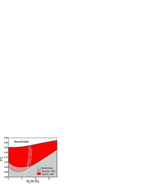
Figure 13: (Color online) Transition temperatures $T_{\text{vav}}$, $T_{\text{vav-symm}}$, $T_{\text{S/N}}$ vs. the size of the hole for a square of sizes $10\xi_{0}\times 10\xi_{0}$ and an applied field of $\phi/\phi_{0}=5.0$. The corners of the holes are at a distance $d_{h}/D=25\%$. On the left side of the white line, the vortices are captured by the holes, on the right side they are outside the holes. $\kappa=1.5$

In the non-linear theory we will now review the role played by the hole size. In Fig. 13 a phase diagram shows the dependence of the VAV stability temperature interval of the hole size. In this figure we used $\kappa=1.5$ and the total applied flux $\phi$ equals $5.0\phi_{0}$. The position of the inner corner of the holes was fixed at $d_{h}/D=25\%$. Although increasing the hole size, enhances the characteristic observables $|\psi|_{max}^{2}$ and $\Delta B_{vav}$ and as well stabilizes against all kinds of defects, we notice one backdraw of large holes: the VAV temperature interval shrinks. One can also see that the VAV temperature interval reaches a maximum size at about $w_{h}/W=5\%$ while the temperature range of asymmetric VAV states remains almost unaltered before this maximum.

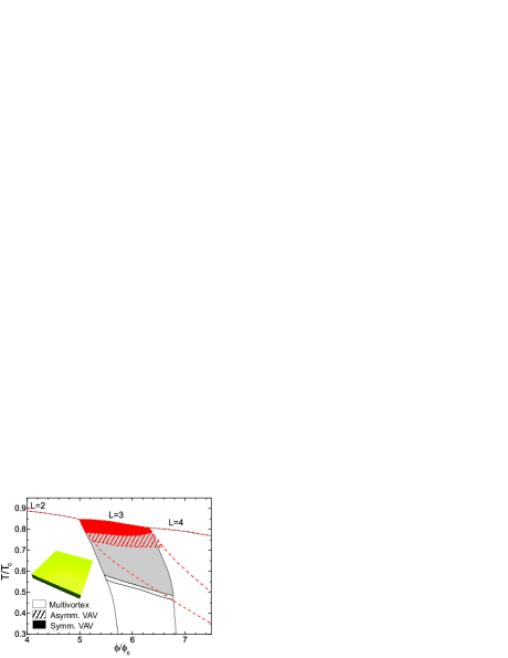
Figure 14: (Color online) $\phi-T$ phase diagram for a plain square, illustrating the ground state regime of the L=3 state. Grey represents $\kappa=\infty$, red (dark grey) $\kappa=1$.

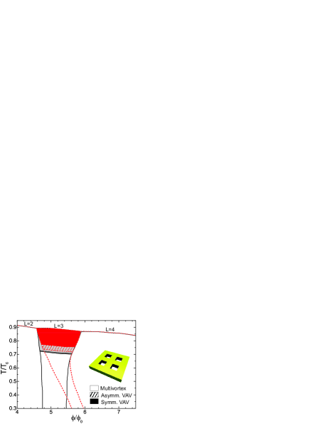
Figure 15: (Color online) $\phi-T$ phase diagram for a square containing four symmetrically placed nanoholes, illustrating the ground state regime of the L=3 state. Grey represents $\kappa=\infty$, red (dark grey) $\kappa=1$. Hole parameters: $w_{h}/W=12.5\%$ and $d_{h}/D=25\%$.

$\phi-T$ phase diagrams are shown in Fig. 14 for a plain square and in Fig. 15 for a perforated square, both of size $10\xi_{0}\times 10\xi_{0}$. Both figures contain two superimposed phase diagrams, one for $\kappa=\infty$ (indicated by grey) and one for $\kappa=1$ (shown in red (dark grey)). The diagrams illustrate the ground state region of the L=3 state, so only the neighboring L=2 and L=4 states are taken into account.

Comparing these two phase diagrams with and without holes, one can clearly see that the introduction of holes of size $w_{h}/W=12.5\%$ at the position $d_{h}/D=25\%$ causes the total VAV region to shrink for a sample with $\kappa=\infty$ but to expand for a sample with $\kappa=1$. Nonetheless, the region of asymmetric VAV states shrinks for both $\kappa$. Note however that this is not true for all sizes. See e.g. Fig. 13 where the asymmetric region initially undergoes a subtle increase.

For both squares a decrease of $\kappa$ leads to: i) a broadening of the temperature regime with an asymmetric vortex state, and ii) it causes a shift of the vorticity to higher fields which is large for low temperatures and smoothly decreases to zero, at the S/N boundary. The reason for the latter is that the larger currents ($j_{s}\propto|\psi|^{2}\propto 1-T/T_{c}$) generate a stronger magnetic field and thus are more effective in expelling and concentrating the magnetic flux. This shift for decreasing $\kappa$ can be understood in the limit to type I superconductivity, where L=0 (i.e. the Meissner state) is the only stable state. The S/N boundary of both $\kappa$ coincide, since at the S/N boundary the second equation does not have an influence.

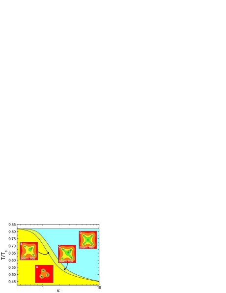
Figure 16: (Color online) $\kappa$-$T$ phase diagram showing the regions where symmetric (cyan/dark grey), asymmetric (shaded) and no antivortex (yellow/light grey) states can be found. Plain square 10$\xi_{0}$ $\times$ 10$\xi_{0}$. Flux $\phi/\phi_{0}=6.$ Insets show contour plots of the logarithm of the CPD for the three regions.

Fig. 16 depicts the $\kappa$-dependence of the temperature-interval wherein the (asymmetric) VAV state is stable in a plain square. It seems that the T-interval of the asymmetric VAV state grows for decreasing $\kappa$. Also it is shown that the decrease of $\kappa$ disfavours the vortex-antivortex nucleation, which is opposite to the findings of Ref. slava where this conclusion was made for a mesoscopic type-I triangle.

For low $\kappa^{*}$, the supercurrents generate a magnetic field which contributes to the total magnetic field and destroys its homogeneity. Obviously, the shape of the magnetic field shows strong similarities with that of the Cooper pair density, which could be the reason for the stabilization of asymmetric VAV states for low $\kappa^{*}$.

From this point of view we can also interpret the broadening of the stability region of asymmetric VAV states for small $\kappa$. The decrease of $\kappa$ acts similarly as having a defect, but one without preferential spatial direction. It only slows the nucleation/annihilation of the VAV pair.

Since the vortex-antivortex state already is a state which is rather unstable and sensitive to all kinds of defects, it is normal that this subtle equilibrium of the coexistence of vortex and antivortex disappears and that the VAV pair annihilates.

From a theoretical viewpoint, there are several ways to make the second order transition from the highly symmetric VAV state to the multivortex state: by decreasing temperature, the magnetic field or $\kappa$. In all these three scenarios the same transition takes place qualitatively: The antivortex moves towards one of the vortices, they approach and eventually annihilate. This clearly is a manifestation of spontaneous symmetry breaking.

VII How to detect the VAV state?

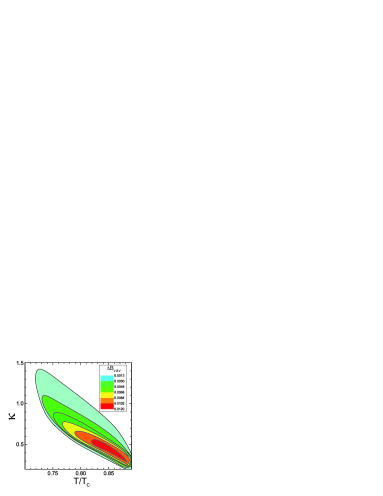
Figure 17: (Color online) Contourplot of the quantity $\Delta B_{VAV}=(B_{V}-B_{AV})/B_{appl}$ as function of $\kappa$ and $T$ for $\phi=5.8$, $T=0.84$ and $\kappa=0.7$ for a $10\xi_{0}\times 10\xi_{0}$ superconducting square with holes. Hole parameters: $w_{h}/W=12.5\%$ and $d_{h}/D=25\%$.

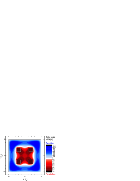
Figure 18: (Color online) Contourplot of the quantity $\Delta B=(B-B_{appl})/B_{appl}$ for $\phi=5.8$, $T=0.84$ and $\kappa=0.7$ in a $10\xi_{0}\times 10\xi_{0}$ superconducting square with holes in the L=4-1 state. Hole parameters: $w_{h}/W=12.5\%$ and $d_{h}/D=25\%$.

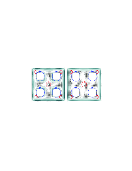
Figure 19: (Color online) The distribution of the supercurrent in a perforated square. The black arrows indicate the direction of the current, the background greyscale map depicts the magnitude of the local supercurrent density (white/black represents low/high). The main characteristics of the current flow pattern are indicated by the blue and red circles. Left: $L=4$ state with applied flux $\phi=7\phi_{0}$. Right: $L=4-1=3$ (VAV) state with applied flux $\phi=5.5\phi_{0}$.

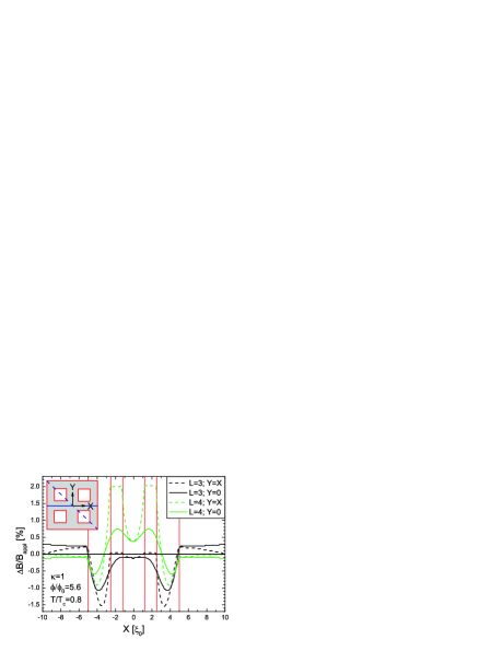
Figure 20: (Color online) Magnetic field profiles (diagonal and vertical cut) for the L=4-1=3 and L=4 states in a perforated square. $\Delta B\equiv B-B_{appl}.$

Essentially, we see two ways to proof experimentally the existence of stable antivortex states: through magnetic field imaging (e.g. using a Hall-probe) and through Cooper pair density imaging (e.g. using Scanning Tunneling Microscopy). In this section we will highlight the advantages and disadventages of both approaches.

An antivortex is characterized by the following properties: i) the CPD in the center is suppressed to be exactly zero, and ii) its supercurrents circulate opposite to the one of the vortices. Unfortunately, the first property also applies to a conventional vortex, so that it cannot be used to discriminate between vortex and antivortex. This means that the magnetic field, generated by the supercurrents, is the only observable parameter able to distinguish between vortex and antivortex.

In our study of superconductors in a homogeneous field, antivortices always seemed to appear surrounded by vortices. However, (multi)vortex currents always generate in the center of the sample an anti-vortexlike current, in a superconducting cog wheels motion of the condensate. This current masks the current profile of a possible antivortex which could be present since it has the same direction. As a consequence, we can not get evidence for the existence of an antivortex by looking in a qualitative way at the magnetic field profile of the sample. As an example, there is no qualitative difference of the supercurrent and the magnetic field profile between the L=4 and L=3 VAV state, as is also shown in Figs. 19 and 20. Of course there is a quantitative difference, which could be exploited.

Nonetheless, one can make use of qualitative differences of both the CPD and the magnetic field profile, at different temperatures. Here the challenge is to control the vorticity of the sample and to assure that it stays constant while measuring and sweeping the temperature. This way one can either measure the CPD or the magnetic field profile. At low temperature the magnetic field profile should clearly exhibit the penetration of the field through the three vortices residing in three of the holes, while at a higher temperature the magnetic field should be penetrating the four holes equally, since a VAV pair is then created, one vortex occupying the empty hole.

For a more direct observation of the antivortex, we suggest taking a sample with low effective $\kappa^{*}$ where a gradual second order nucleation of the vortex-antivortex pair is found. Then, using our findings from Sec. VI, subsequent CPD images for slowly increasing/decreasing temperature or magnetic field should demonstrate clear evidence for VAV-nucleation/annihilation. In this scenario, the hole parameters have to be chosen to maximize the stability region of asymmetric VAV states in the vortex-phase diagram, following the guidelines from the preceding section.

VIII Conclusions

The existence of geometry induced antivortices in the presence of a homogeneous magnetic field has been predicted theoretically several years ago VAVNature . Up to now, there does not exist any experiment with the observation of it. With numerical simulations, using both the linear and full non-linear Ginzburg-Landau theory, we investigated how to engineer superconducting samples to stabilize and enhance the antivortex.

We propose how to engineer the superconducting sample but without taking away the conceptual novelty of the nucleation of the vortex-antivortex pair in a homogeneous magnetic field, as opposed to the idea of placing e.g. a magnetic dot on top of the sample. We pursued the idea to introduce holes which will act as pinning centers, and in doing so, pull the vortices away from the anti-vortex and additionally to provide a strong immunity against imperfections and defects. First we elaborated on the size and position of these holes. We determined optimal parameters for the square and triangle geometry. For instance, in a square geometry, we managed to enlarge the separation between vortex and antivortex with a factor 4, compared to the case without holes.

We investigated the influence of several kinds of geometrical defects on the VAV state. For all the imperfections we studied, we found that the holes cause a substantial increase of the stability of the VAV configuration with respect to defects. With the technology which is nowadays available it is possible to manufacture samples with the desired precision to proof the existence of VAV states.

The geometry induced antivortices are known to be a consequence of the symmetry of the sample. Therefore, we focussed on the competition of different sources of symmetry in the mesoscopic superconductor. We concluded that the pinning centers are by far the most efficient in imposing their symmetry, while the role of the outer boundary of the sample has a less determining role. Thinking further on this line, we studied circular disks, perforated by a number of symmetrically placed holes, and found giant antivortices up to a vorticity of -7. However, we found that this spectacular configuration, is highly sensitive to imperfections.

The effect of the non-linearity of the first GL equations and the magnetic screening represented by the second GL equation was critically examined, allowing us to investigate the influence of temperature and non-zero thickness of the sample on the VAV state.

We constructed phase diagrams for different values of $\kappa$ for the perforated and the plain square system showing the stability region of the VAV state in the $\phi-T$ plane. For low value of $\kappa$ the introduction of holes enlarges the stability region. We also found the remarkable appearance of asymmetric VAV states, stable in a wide region of the phase diagram. Such asymmetric states are counterintuitive since the VAV state is known to be a consequence of symmetry and yet manifests in an asymmetric way because of the important non-linearity of the GL equations. Nevertheless, the existence of asymmetric VAV states can be the key property for an experiment to proof the existence of VAV states. We revisited our discussion about the hole size in this new context and found out that the size of the holes has a large influence on the stability region of the asymmetric states.

We showed that a small value of $\kappa^{*}$ disfavors the vortex-antivortex state in all investigated geometries (square, perforated square, perforated triangle), indicating that the findings of Ref. slava where a vortex-antivortex state in a type-I triangle is predicted with large VAV-separation cannot be correct. We mainly concentrated our discussion on square samples but we believe that the main conclusions are also valid for triangle samples.

IX Acknowledgements

This work was supported by the Flemish Science Foundation (FWO-Vl), the Belgian Science Policy, the JSPS/ESF-NES program, and the ESF-AQDJJ network.

References

- (1) L.F. Chibotaru, A. Ceulemans, V. Bruyndoncx, and V.V. Moshchalkov, Nature (London) 408, 833 (2000).
- (2) J. Bonča and V.V. Kabanov, Phys. Rev. B 65, 012509 (2002).
- (3) T. Mertelj and V.V. Kabanov, Phys. Rev. B 67, 134527 (2003).
- (4) L.F. Chibotaru, G. Teniers, A. Ceulemans, and V.V. Moshchalkov, Phys. Rev. B 70, 094505 (2004).
- (5) A.S. Mel’nikov, I.M. Nefedov, D.A. Ryzhov, I.A. Shereshevskii, V.M. Vinokur, and P.P. Vysheslavtsev, Phys. Rev. B 65, 140503 (2002).
- (6) C. Carballeira, V.V. Moshchalkov, L.F. Chibotaru, and A. Ceulemans, Phys. Rev. Lett. 95, 237003 (2005).
- (7) M.V. Milošević and F.M. Peeters, Phys. Rev. Lett. 93, 267006 (2004); ibid. Phys. Rev. Lett. 94, 227001 (2005).
- (8) R. Geurts, M. V. Milošević, and F. M. Peeters, Phys. Rev. Lett. 97, 137002 (2006).
- (9) L.F. Chibotaru, A. Ceulemans, V. Bruyndoncx, and V. V. Moshchalkov, Phys. Rev. Lett. 86, 1323 (2001)
- (10) L.F. Chibotaru, A. Ceulemans, G. Teniers, and V.V. Moshchalkov, Physica C 369, 149-157 (2002).
- (11) R. Kato, Y. Enomoto, and S. Maekawa, Phys. Rev. B 47, 8016 (1993)
- (12) V.R. Misko, V.M. Fomin, J.T. Devreese, and V.V. Moshchalkov, Phys. Rev. Lett. 90, 147003 (2003).
- (13) V.A. Schweigert and F.M. Peeters, Phys. Rev. B 57, 13817 (1998); P.S. Deo, V.A. Schweigert, F.M. Peeters, and A.K. Geim, Phys. Rev. Lett. 79, 4653 (1997).
- (14) R. Prozorov, E.B. Sonin, E. Sheriff, A. Shaulov, and Y. Yeshurun, Phys. Rev. B 57, 13845 (1998).
- (15) M. Tinkham, Introduction to Superconductivity (McGraw Hill, New York, 1975).
- (16) G.R. Berdiyorov, B.J. Baelus, M.V. Milošević, and F.M. Peeters, Phys. Rev. B 68, 174521 (2003).
- (17) A.K. Geim, S.V. Dubonos, I.V. Grigorieva, K.S. Novoselov, F.M. Peeters, and V.A. Schweigert, Nature (London) 407, 55 (2000).
- (18) F.M. Peeters, B.J. Baelus, and V.A. Schweigert, Physica C 369, 158 (2002)
- (19) B.J. Baelus, K. Kadowaki, and F.M. Peeters, Phys. Rev. B 71, 024514 (2005).