Routes to synchrony between asymmetrically interacting oscillator ensembles

Abstract

We report that asymmetrically interacting ensembles of oscillators (AIEOs) follow novel routes to synchrony. These routes seem to be a characteristic feature of coupling asymmetry. We show that they are unaffected by white noise except that the entrainment frequencies are shifted. The probability of occurrence of the routes is determined by phase asymmetry. The identification of these phenomena offers new insight into synchrony between oscillator ensembles and suggest new ways in which it may be controlled.

Coupling asymmetry between oscillators is widespread in real physical and biological systems. Examples include cardio-respiratory and cardio-$\delta$(EEG) interactions Stefanovska:07 , interactions among activator-inhibitor systems Daido:06 , coupled circadian oscillators Fukuda:07 , and the interactions between ensembles of oscillators in neuronal dynamics Sherman:92 ; Roelfsema:97 . Synchrony can be sometimes be desirable as in e.g. lasers and Josephson-Junction arrays Trees:05 , or temporal coding and cognition via brain waves Singer:99 ; but it can also be dangerous, as in epileptic seizures Timmermann:03 , Parkinson’s tremor Percha:05 , or pedestrians on the Millennium Bridge Strogatz:01 . Thus the control of synchronization Blasius:03 can often be important. An understanding how synchrony arises is of course an essential prerequisite for the development of control schemes.

In this Letter, we report a phenomenon that occurs in asymmetrically interacting ensembles of oscillators (AIEOs), where it provides novel routes to synchrony. These routes are the characteristic of AIEOs and they cannot occur in systems where the interactions are symmetrical. Our results yield new insights into how synchrony arises and offer possible ways of controlling synchrony between real AIEOs.

The phase dynamical equations of a system of two AIEOs can be written as Kuramoto:84

$$\dot{\theta_{i}}^{(1,2)} = \omega_{i}^{(1,2)}-\frac{A^{(1,2)}}{N^{(1,2)}}\sum_{j=1}^{N^{(1,2)}}\sin(\theta_{i}^{(1,2)}-\theta_{j}^{(1,2)}+\alpha^{(1,2)})$$ (1)

$$\quad-\frac{B}{N^{(2,1)}}\sum_{j=1}^{N^{(2,1)}}\sin(\theta_{i}^{(1,2)}-\theta_{j}^{(2,1)}+\alpha^{3}).$$

The interactions are characterized by coupling parameters $A^{(1,2)}$ and $B$ to quantify respectively the interactions within, and between, the ensembles. The fact that $A^{(1)}\neq A^{(2)}$ (c–asymmetry hereafter) implies that the oscillators in the ensembles are asymmetrically coupled. $\theta_{i}^{(1,2)}$ are the phases of the $i$th oscillator in each ensemble and $N^{(1,2)}$ refer to the ensemble sizes; we take $N^{(1)}=N^{(2)}=N$, with $N\rightarrow\infty$. Phase asymmetry (p–asymmetry hereafter) is introduced by phase shifts $0\leq\alpha^{(1,2,3)}<\pi/2$. The natural oscillator frequencies $\omega_{i}^{(1,2)}$ are assumed to be Lorentzianly distributed as $g(\omega^{(1,2)})=\frac{\gamma}{\pi}(\gamma^{2}+(\omega-\bar{\omega}^{(1,2)})^{2})^{-1}$ with central frequencies $\bar{\omega}^{1,2}$, and $\gamma$ is the half–width at half–maximum. With this characterization, we show that an increase of the coupling strength between two ensembles that are synchronized separately does not immediately result in their mutual phase-locking. Rather, phase-locking occurs through either one of two different routes: in Route-I the oscillators in the two ensembles combine and form clusters; in Route-II one of the ensembles desynchronizes while the other remains synchronized. Further, there also exists the possibility that phase-locking between the ensembles cannot occur at all.

The model can conveniently be expressed in terms of (complex-valued, mean-field) order parameters $r^{(1,2)}e^{i\psi^{(1,2)}}=\frac{1}{N}\sum_{j=1}^{N}e^{i\theta_{j}^{(1,2)}}$. Here $\psi^{(1,2)}(t)$ are the average phases of the oscillators in the respective ensembles and $r^{(1,2)}(t)$ provide measures of the coherence of each oscillator ensemble which varies from 0 to 1. When $r^{(1,2)}\approx 1$ the corresponding ensemble is synchronized in phase (microscopic synchronization) and when $\delta\psi=\psi^{(1)}-\psi^{(2)}\approx$ constant the ensembles are mutually locked in phase (macroscopic synchronization). With these definitions, Eq. (1) becomes

$$\dot{\theta_{i}}^{(1,2)} = \omega_{i}^{(1,2)}-A^{(1,2)}r^{(1,2)}\sin(\theta_{i}^{(1,2)}-\psi^{(1,2)}+\alpha)$$ (2)

$$\quad-Br^{(2,1)}\sin(\theta_{i}^{(1,2)}-\psi^{(2,1)}+\alpha),$$

where for simplicity we have considered the particular case $\alpha^{(1,2,3)}=\alpha$. In the limit $N\rightarrow\infty$, a density function can be defined as $\rho^{(1,2)}(\theta,t,\omega)d\omega d\theta$ which describes the number of oscillators with natural frequencies within $[\omega,\omega+d\omega]$ and with phases within $[\theta,\theta+d\theta]$ at time $t$. For fixed $\omega$ the distribution $\rho^{(1,2)}(\theta,t,\omega)$ obeys the evolution equation $\partial\rho^{(1,2)}/\partial t=-\partial(\rho^{(1,2)}\dot{\theta}^{(1,2)})/\partial\theta$. The function $\rho^{(1,2)}(\theta,t,\omega)$ is real and $2\pi$ periodic in $\theta$, so it can be expressed as a Fourier series in $\theta$

$$\rho^{(1,2)}(\theta,t,\omega) = \sum_{l=-\infty}^{\infty}\rho_{l}^{(1,2)}(\omega,t)e^{il\theta}$$

$$= \frac{1}{2\pi}+\rho_{1}^{(1,2)}e^{i\theta}+\mbox{c.c}+\eta(\theta,t,\omega),$$

where c.c is the complex conjugate of the preceding term and $\eta(\theta,t,\omega)$ denotes the 2nd and higher harmonics. Substituting $\rho^{(1,2)}(\theta,t,\omega)$ into the evolution equation, we get the following linearized equation for $\rho_{1}$ as

$$\dot{\rho_{1}}^{(1,2)} + i\omega\rho_{1}^{(1,2)}=\frac{e^{i\alpha}}{2}\left(A^{(1,2)}\langle\rho_{1}^{(1,2)}\rangle+B\langle\rho_{1}^{(2,1)}\rangle\right),$$ (3)

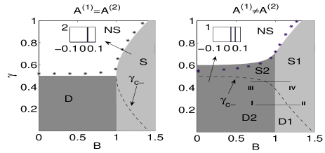
Figure 1: ($B$–$\gamma$) bifurcation diagram for $\alpha=0,\Delta\omega=1$. The different synchronization regimes are described in the text. The boundary between regimes NS and S/D represents $\gamma_{c+}$. The $*$s represent the numerical bifurcation boundaries; (left) $A^{(1)}=A^{(2)}=1$, (right) $A^{(1)}=1.2,A^{(2)}=1$. Insets show the frequency distributions (also obtained numerically) for the indicated regions; their ordinate axes represent oscillator counts in thousands. Note that the occurrence of perfect synchronization with $2000$ (left) and $1000$ (right) oscillator groups will not occur throughout all of each indicated region.

where the Fourier components for $|l|\geq 2$ are neglected since $l=\pm 1$ are the only nontrivial unstable modes and $\rho_{0}=1/2\pi$ is the trivial solution corresponding to incoherence. $\langle\cdot\rangle$ represents the average over the frequencies $\omega^{(1,2)}$ weighted by the Lorentzian distribution $g(\omega^{(1,2)})$. The eigenvalues obtained from the characteristic equation of (3) are

$$\lambda_{\pm}=\left\{\begin{array}[]{ll}-\gamma+\frac{\kappa}{4}e^{i\alpha}\pm\frac{1}{2}(p^{2}+q^{2})^{\frac{1}{4}}e^{i\frac{1}{2}\zeta}-i\bar{\omega},&\\ \qquad\qquad\qquad\qquad\qquad\qquad\qquad p>0&\\ \\ -\gamma+\frac{\kappa}{4}e^{i\alpha}\mp\frac{i}{2}(p^{2}+q^{2})^{\frac{1}{4}}e^{i\frac{1}{2}\zeta}-i\bar{\omega},&\\ \qquad\qquad\qquad\qquad\qquad\qquad\qquad p<0&\end{array}\right.$$ (9)

where $\kappa=A^{(1)}+A^{(2)}$, $\xi=(\frac{1}{4}\hat{A}^{2}+B^{2})$, $\hat{A}=(A^{(1)}-A^{(2)})$, $\zeta=\tan^{-1}(\frac{q}{p})$, $\Delta\omega=\bar{\omega}^{(1)}-\bar{\omega}^{(2)}$, $\bar{\omega}=(\bar{\omega}^{(1)}+\bar{\omega}^{(2)})/2$, $p=\xi\cos(2\alpha)+\hat{A}\Delta\omega\sin{\alpha}-\Delta\omega^{2}$, and $q=\xi\sin(2\alpha)-\hat{A}\Delta\omega\cos{\alpha}$. As a signature of synchronization, we take the condition $Re(\lambda_{\pm})>0$ for analytic treatment. For the numerical experiment, we set $r^{(1,2)}>0.7$ for microscopic synchronization in the corresponding ensembles and a constant $\delta\psi$ for macroscopic synchronization as the conditions. We take $N=1000$ in each ensemble and the equations are solved using a fourth-order Runge–Kutta routine. The initial phases of the oscillators are assumed to be equally distributed in $[0,2\pi)$.

One might intuitively anticipate the possibility of four distinct dynamical regimes: no synchronization (NS); global synchronization, in which the oscillators of both ensembles are entrained to the same frequency (S1); synchronization within one ensemble but not the other (S2); synchronization within both ensembles, separately and independently, with two entrainment frequencies (D2). In what follows, we show that this is indeed the case and, furthermore, that there is a global regime in which the two ensembles behave as one, but oscillators within each ensemble are entrained at either one of two distinct entrainment frequencies (D1). Regions S2 and D1 cannot occur when c–asymmetry is absent Okuda:91 (see Fig. 1).

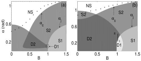
Figure 2: ($B$–$\alpha$) bifurcation diagram for (a) $A^{(1)}=1.2,A^{(2)}=1$, (b) $A^{(1)}=1.8,A^{(2)}=1.4$ and $\Delta\omega=1,\gamma=0.5$. Note that the synchronization regimes S1 and D1 are greatly reduced in the presence of p–asymmetry. The $*$s denote the numerical bifurcation boundary between the synchronized and incoherent states. The discrepancy between numerical and analytical boundaries occurs due the p–asymmetry (unlike Fig. 1) that affects region S2 and hence the thresholds for $r^{(1)}$ and $r^{(2)}$.

For the case $\alpha=0$, when $p>0$, in the region S1, the incoherent (steady) state becomes unstable via a single Hopf bifurcation and the ensembles entrain to a single frequency $\Omega_{+}$. With further decrease of $\gamma$ below the $\gamma_{c-}$ line in the region D1, a new entrainment frequency emerges through a second Hopf bifurcation. In this region, the oscillators from the two ensembles combine and form two clusters (macroscopic clustering) oscillating with two frequencies, $\Omega_{\pm}=-\mbox{Im}(\lambda_{\pm})=\pm(1/2)[p^{2}+q^{2}]^{\frac{1}{4}}\sin{(\frac{1}{2}\zeta)}+\bar{\omega}$. $\gamma_{c\pm}$ are obtained by imposing the condition $Re(\lambda_{\pm})=0$. Thus in this region the order parameters either fluctuate in a quasi–periodic manner or have complicated dynamics (see Fig. 3). This is because each ensemble has two clusters oscillating with different frequencies (see Figs. 3(a) and 4) 01 . The presence of two entrainment frequencies can be seen by looking at the frequencies into which all the individual oscillators are grouped as shown in Fig. 4. The macroscopic clustering that occurs in this case is quite different from formation of clusters in a single ensemble Kuramoto:84 ; Golomb - here the oscillators in two different ensembles combine and form clusters. The occurrence of this phenomenon provides new insight into the control of synchrony in realistic situations where there is asymmetry, like neural networks where neurons from one ensemble (e.g. cortex) tend to synchronize with those in the other ensemble (e.g. thalamus) thus giving rise to creating desirable or undesirable (e.g. epileptic seizures) effects. In the absence of coupling asymmetry, these phenomena do not exist. Traversing the line I–II of Fig. 1 demonstrates Route–I to phase-locking of the ensembles. As we increase $B$, the oscillators in the ensembles pass from the dynamical state of microscopic synchronization (D2) through macroscopic clustering to macroscopic synchronization or phase-locking of the ensembles. Note that when $A^{(1)}=A^{(2)}$ or $\Delta\omega=0$ only one entrainment frequency exists below $\gamma_{c-}$ and therefore this sequence does not occur (due to the absence of region D1). While traversing the line III-IV of Fig. 1 the ensembles adopt Route-II to phase-locking in which it is the macroscopic clustering that does not occur.

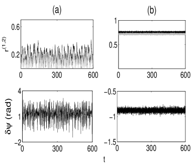
Figure 3: Numerical plot of coherence parameters $r^{(1)}$ (grey), $r^{(2)}$ (black) and phase difference $\delta\psi$ as a function of time. Here (a) $B=1$, $\alpha=0.23$ and (b) $B=1$, $\alpha=0.47$. (a) and (b) correspond to regions D1 and D2 of Fig. 2(b) for the same values of parameters as traveling along the line $I-II$. Note that the order parameters display no synchronization in the D1 region.

When $p<0$, corresponding to regions S2 and D2 in Fig. 1, the dynamics is the same as above except that the values of critical $\Gamma$ and synchronization frequencies differ, as can be calculated from Eq. (9). In region S2, microscopic synchronization can occur in either one of the ensembles, depending upon whether $A^{(1)}$ or $A^{(2)}$ is greater; in Fig. 1, since $A^{(1)}>A^{(2)}$, synchronization occurs in the first ensemble with the second ensemble remaining incoherent. Note that, on increasing $B$ while in region S2, the condition $p<0$ is violated and the ensembles enter into the phase-locked region S1. In region D2, the ensembles synchronize separately to two locking frequencies (unlike in region D1 where the ensembles combine). The corresponding $(B-\gamma)$ bifurcation diagram for the case $A^{(1)}$=$A^{(2)}$ is plotted in Fig. 1 (left) to show the difference between these two cases. The region D represents microscopic synchronization which occurs through a degenerate Hopf bifurcation (similar to D2) and S represents macroscopic synchronization through a single Hopf bifurcation (similar to S1). The regions S2 and D1 cannot arise for this case. Hence the ensembles cannot follow either Route-I or Route-II to synchrony but can only pass from the dynamical states of microscopic synchrony to macroscopic synchrony.

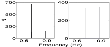
Figure 4: Histograms showing virtual desynchronization - Left: First ensemble, Right: Second ensemble, for the corresponding parameter values in Fig. 3 (a). Note that the first frequency component in both the ensembles have two indistinguishably different subcomponents which may be considered as one. This occurs due to the discrepancy between numerics and analytics.

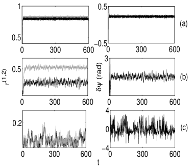
Figure 5: Numerical plot of coherence parameters $r^{(1)}$ (grey), $r^{(2)}$ (black) and phase difference $\delta\psi$ as a function of time. (a) $B=0.7,\alpha=0.2$ (b) $B=0.7,\alpha=\pi/4$ (near $\alpha_{c}$) (c) $B=0.7,\alpha=1.2$ ($\alpha>\alpha_{c}$). (a), (b) and (c) correspond to regions D2, near NS/S2 boundary and NS of Fig. 2(a) for the same values of parameters.

For the case $\alpha\neq 0$, regions D1 and S1 shrink as $\alpha$ increases, whereas S2 expands, as shown in Fig. 2. This means that p–asymmetry reduces the probability of macroscopic synchronization (reduced S1 and D1 regions in Fig. 2) and mostly allows only microscopic synchronization of one or both of the ensembles. For a given set of parameters, there exists a value of $\alpha$ below which the condition $p>0$ is satisfied and above which $p<0$ is satisfied. As a result, when $\alpha>\alpha_{j}$ the macroscopic synchrony breaks and the system enters the microscopically synchronized state. Thus as one travels from S1 (D1) to S2 (D2) across $\alpha_{j}$ the combined synchrony with single (double) frequency breaks between the ensembles and independent synchronization with single (double) frequency regime appears. Region S2, unlike in Fig. 1, embraces two states (i) synchronization in ensemble 1 with ensemble 2 incoherent and (ii) synchronization in ensemble 2 with ensemble 1 incoherent, but does distinguish between them. Further, there is a critical value of $\alpha=\alpha_{c}$ above which the collective oscillations disappear and the incoherent state becomes stabilized (see Figs. 2 and 5).

Real physical systems are of course subject to noise (random fluctuations, of either internal or external origin), so we now consider how the above analysis will be modified as a result. Adding $\eta_{i}^{(1,2)}$ to the RHS of Eq. (1), where $\eta_{i}^{(1,2)}$ are independent Gaussian white noises with $\langle\eta_{i}^{(1,2)}(t)\rangle=0$ and $\langle\eta_{i}^{(1,2)}(t)\eta_{j}^{(1,2)^{\prime}}(t)\rangle=2K^{(1,2)}\delta(t-t^{\prime})\delta_{ij}$ and $K^{(1,2)}$ are the noise intensities, the eigenvalues of the linearized equation then take the form

$$\lambda_{\pm}=\left\{\begin{array}[]{ll}-\bar{K}-\gamma+\frac{\kappa}{4}e^{i\alpha}\pm\frac{1}{2}(p^{2}+q^{2})^{\frac{1}{4}}e^{i\frac{1}{2}\zeta}-i\bar{\omega},&\\ \qquad\qquad\qquad\qquad\qquad\qquad\qquad p>0&\\ \\ -\bar{K}-\gamma+\frac{\kappa}{4}e^{i\alpha}\pm\frac{i}{2}(p^{2}+q^{2})^{\frac{1}{4}}e^{i\frac{1}{2}\zeta}-i\bar{\omega},&\\ \qquad\qquad\qquad\qquad\qquad\qquad\qquad p<0&\end{array}\right.$$ (15)

where $\bar{K}=\frac{(K^{(1)}+K^{(2)})}{2}$, $\Delta K=K^{(1)}-K^{(2)}$ $p=\xi\cos(2\alpha)+\hat{A}[\Delta\omega\sin{\alpha}+\Delta K\cos(\alpha)]-\Delta\omega^{2}+\Delta K^{2}$ and $q=\xi\sin(2\alpha)-\hat{A}\Delta\omega\cos{\alpha}-\hat{A}\Delta K\sin{\alpha}+2\Delta\omega\Delta K$. For simplicity, if we consider $K^{(1)}=K^{(2)}=K$, one can then replace $\gamma$ in Eq. (9) by $\gamma+K$. Thus from Eq. (15) it is evident that the dynamics and hence the new route to synchrony are unaffected by the presence of white noise. Consequently, for increasing noise intensity, the incoherent state becomes unstable for larger values of the critical parameters. When $K^{(1)}\neq K^{(2)}$ the entrainment frequency depends on $\Delta K$ (shown in Fig. 6). On increasing $\Delta K$ ($K^{(1)}>K^{(2)}$), the microscopic synchronization of ensemble 1 is destroyed.

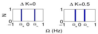
Figure 6: The shift in the entrainment frequencies $\Omega_{\pm}$ with $\Delta K$. Here $A^{(1)}=A^{(2)}$, $B=0.5$, $\alpha=0$, $\bar{\omega}=0$ and $\Delta\omega=1$. $N$ represents oscillator count in thousands.

In summary, we have found new routes to synchrony between two AIEOs, characterized by asymmetry in the coupling strength. We have also established that the effect of white noise is simply to alter the critical values of the parameters that control bifurcation, and to change the entrainment frequencies, but without otherwise affecting this route to synchrony. Our main focus has been on phase oscillator ensembles, but similar phenomena can also be identified in ensembles of other kinds of oscillators.

The authors are indebted to A. Bahraminasab, D. Garcia-Alvarez and M. G. Rosenblum for valuable discussions. The study was supported by the EC FP6 NEST-Pathfinder project BRACCIA and in part by the Slovenian Research Agency and the Council of Scientific and Industrial Research, India.

References

- (1) B. Musizza, A. Stefanovska, P. V. E. McClintock, M. Palus, J. Petrovcic, S. Ribaric, F. F. Bajrovic, J. Physiol. (London) 580, 315 (2007).
- (2) H. Daido, K. Nakanishi, Phys. Rev. Lett. 96, 054101 (2006); 93, 104101 (2004);Phys. Rev. E. 75, 056206 (2007); I. Z. Kiss, Y. M. Zhai, J. L. Hudson, Science 296, 1676 (2002).
- (3) H. Fukuda, N. Nakamichi, M. Hisatsune, H. Murase, and T. Mizuno, Phys. Rev. Lett. 99, 098102 (2007).
- (4) A. Sherman, J. Rinzel, Proc. Natl. Acad. Sci. U.S.A. 89, 2471 (1992).
- (5) P. R. Roelfsema, A. K. Engel, P. Konig and W. Singer, Nature 385, 6612 (1997); W. Singer, Nature 397, 6718 (1999).
- (6) B. Blasius, E. Montbrio, J. Kurths, Phys. Rev. E. 67, 035204(R) (2003); E. Montbrio and B. Blasius, Chaos 13, 291 (2003); B. Blasius, Phys. Rev. E. 72, 066216 (2005).
- (7) B. R. Trees, V. Saranathan, D. Stroud, Phys. Rev. E 71, 016215 (2005); F. Rogister, R. Roy, Phys. Rev. Lett. 98 104101 (2007).
- (8) W. Singer, Neuron 24 49 (1999); P. Fries, Trends. Cogn. Sci. 9 474 (2005);Y. Yamaguchi, N. Sato, H. Wagatsuma, Z. Wu, C. Molter and Y. Aota, Curr. Opin. Neurobiol. 17, 197 (2007).
- (9) L. Timmermann, J. Gross, M. Dirks, J. Volkmann, H. Freund and A. Schnitzler Brain 126, 199 (2003),J. A. Goldberg, T. Boraud, S. Maraton, S. N. Haber, E. Vaadia, and H. Bergman, J. Neurosci. 22, 4639 (2002)
- (10) B. Percha, R. Dzakpasu, and M. Zochowski, Phys. Rev. E. 72, 031909 (2005); M. Zucconi, M. Manconi, D. Bizzozero, F. Rundo, C. J. Stam, L. Ferini-Strambi, R. Ferri, Neurol. Sci. 26 199 (2005).
- (11) S. H. Strogatz, Nature 410, 268 (2001).
- (12) Y. Kuramoto, Chemical Oscillations, Waves, and Turbulence (Springer-Verlag, Berlin, 1984); A. Pikovsky, M. Rosenblum, and J. Kurths, Synchronization – A Universal Concept in Nonlinear Sciences (Cambridge University Press, Cambridge, 2001).
- (13) K. Okuda and Y. Kuramoto, Prog. Theor. Phys. 86, 1159 (1991); E. Montbrio, J. Kurths, and B. Blasius, Phys. Rev. E 70, 056125 (2004).
- (14) Even though Figs. 3 and 4 are plotted for the case , they still describe quite well cases where . This is because finite does not change the dynamical behavior in region D1, though it does changes the size of this region.
- (15) D. Golomb, D. Hansel, B.Shraiman, H. Sompolinsky, Phys. Rev. A 45, 3516 (1992) U. Ernst, K. Pawelzik, T. Geisel, Phys. Rev. Lett. 74 1570 (1995); P. Tass, Phys. Rev. E 56, 2043 (1997); Y. C. Kouomou and P. Woafo, Phys. Rev. E 67, 046205 (2003); R. E. Amritkar, S. Jalan and H. Chin-Kun, Phys. Rev. E 72, 016212 (2005).