Weak and strong measurement of a qubit using a switching-based detector

Abstract

We analyze the operation of a switching-based detector that probes a qubit’s observable that does not commute with the qubit’s Hamiltonian, leading to a nontrivial interplay between the measurement and free-qubit dynamics. In order to obtain analytic results and develop intuitive understanding of the different possible regimes of operation, we use a theoretical model where the detector is a quantum two-level system that is constantly monitored by a macroscopic system. We analyze how to interpret the outcome of the measurement and how the state of the qubit evolves while it is being measured. We find that the answers to the above questions depend on the relation between the different parameters in the problem. In addition to the traditional strong-measurement regime, we identify a number of regimes associated with weak qubit-detector coupling. An incoherent detector whose switching time is measurable with high accuracy can provide high-fidelity information, but the measurement basis is determined only upon switching of the detector. An incoherent detector whose switching time can be known only with low accuracy provides a measurement in the qubit’s energy eigenbasis with reduced measurement fidelity. A coherent detector measures the qubit in its energy eigenbasis and, under certain conditions, can provide high-fidelity information.

I Introduction

The quantum theory of measurement is of particular significance in the study of physics because it lies at the boundary between the quantum and classical worlds Zurek . Quantum measurement has received renewed attention recently from a new perspective, namely its role in quantum information processing Nielsen . Understanding how the quantum state evolves during the measurement process and the information that can be extracted from the raw measurement data is crucial for optimizing the design and operation of measurement devices.

One typically thinks of the measurement process in terms of the instantaneous, projective measurement encountered in the study of basic quantum phenomena. For example, one sometimes imagines that at any desired point in time the spin of a particle can be measured along any desired axis. In many situations, however, the measurement device is weakly coupled to the quantum system being measured, such that the latter evolves almost freely according to its free Hamiltonian while being barely perturbed by the measuring device.

In the context of solid-state quantum information processing, the weak coupling between the qubit and the measuring device is imposed by the need to minimize the decoherence of the qubit before the measurement; in practice it is not possible to completely decouple the qubit from the measuring device, even before the measurement is performed. It is worth mentioning here that although this constraint of weak coupling might seem to be undesirable for measurement purposes, weak coupling between the qubit and the measuring device can have advantages over strong coupling. For example, when the energy eigenstates of a multi-qubit system contain some residual entanglement between the qubits, this entanglement translates into errors when using strong single-qubit measurements, whereas weak coupling to the measuring device can lead to a measurement that is protected from such errors Ashhab .

In the study and implementation of qubit-state readout, one strategy to remove any conflict between the qubit’s free dynamics and the measurement process has been to bias the qubit at a point where the qubit Hamiltonian and the operator being probed by the measuring device commute. In this case the free qubit dynamics conserves the quantity being measured. This dynamics can therefore be ignored during the measurement process, and the only difference between weak and strong qubit-detector coupling is in the amount of time needed to obtain a high-fidelity measurement result. It should be noted, however, that in practice it is not always possible to reach such an ideal bias point.

Here we are mainly interested in the analysis of the measurement process when the qubit Hamiltonian and the operator being probed by the measuring device do not commute. One must therefore analyze the simultaneous working of two physical processes that, in some sense, push the qubit in different directions. We shall focus on the experimentally relevant example of a binary-outcome switching-based measuring device (i.e. the situation where the measuring device can switch from its initial state, to which we refer as 0, to another state, called 1, depending on the state of the qubit), mainly as applied to superconducting circuits YouReview . Our work has a similar motivation to the recent experimental and theoretical work of Refs. Nakano ; Tanaka . However, that work considered a measurement protocol where the measured quantity is the value of the bias current at which switching occurs, whereas we consider the more common approach that uses the switching probability at fixed bias parameters. Other related recent studies include work on the continuous monitoring of Rabi oscillations Ilichev , as well as the theoretical study in Ref. Wei of multiple linear detectors simultaneously probing different observables of the same qubit. A models similar to ours was also used in Ref. Brun to study certain aspects of quantum state evolution under the influence of weak measurement.

It is worth clarifying from the outset a point concerning terminology. A strong measurement is a measurement whose outcome is strongly correlated with the measured quantity, thus specifying with a high degree of certainty the state of the measured system. After the measurement the system is, to a good approximation, projected onto a state with a well-defined value of the measured quantity. A weak measurement, on the other hand, is a measurement whose outcome is weakly correlated with the measured quantity, thus serving as a weak indicator of the state of the measured system. Under suitable conditions a sequence composed of a large number of weak measurements can result in an effectively strong measurement. A weak measurement can also result in reliable information when repeated a large number of times on identically prepared systems. It is sometimes stated that weak measurement results from weak coupling between the measured system and the measuring device. It should be noted, however, that weak coupling does not necessarily imply a weak measurement. We shall therefore use the terms slow-switching and fast-switching detectors in this paper. This distinction could be understood as being between weak-coupling and strong-coupling measurements. A weak-coupling measurement can result in a weak or strong measurement depending on other system parameters, as we shall show with a number of examples below.

This paper is organized as follows: In Sec. II we describe the model and briefly explain an example demonstrating the operation of the switching-based detector in a simple case. In Sec. III we outline our approach to the analysis of the measurement process when using a detector that has a short coherence time. A number of specific examples are treated in Sec. IV. The case of a detector that has a relatively long coherence time is treated in Sec. V. The results of Secs. II-V are reviewed in Sec. VI. We discuss the relevance of our analysis and results to the readout of superconducting flux qubits in Sec. VII, and we summarize our results in Sec. VIII.

II Model

Figure 1: Schematic diagram of the theoretical model that we use to analyze the operation of a switching-based detector. The qubit’s energy eigenstates are denoted by $\left|0\right\rangle$ and $\left|1\right\rangle$, and they have energy separation $E$. The detector is a two-state system (TSS) [with a non-switched state $\left|N\right\rangle$ and a switched state $\left|S\right\rangle$] that is constantly being monitored by a macroscopic system. The detector probes the operator $\hat{\sigma}_{\bf n}$ of the qubit. $\chi$ represents the detector’s operator through which the detector is coupled to the qubit. The macroscopic system monitors whether the TSS remains in the initially prepared state $\left|N\right\rangle$ or switches to the state $\left|S\right\rangle$.

We consider the situation where one is trying to read out the state of a quantum two-level system, i.e. a qubit. The qubit is placed in contact with a binary-outcome detector, i.e. a detector that produces one of two possible readings. The detector is initialized in one of its two possible outcomes, and it can switch to the other one, depending on the state of the qubit. For a large part of the following analysis, we shall assume that the detector itself is a quantum two-state system that is constantly being monitored by a macroscopic, classical system (see Fig. 1). We shall refer to the non-switched and switched states of the detector as $\left|N\right\rangle$ and $\left|S\right\rangle$, respectively. Although the two-state-detector model does not accurately describe the realistic measuring devices that we shall discuss in Sec. VII, this simplification in the model will allow us to carry out our calculations analytically and obtain a good amount of insight into the dynamics of the measurement process. We shall come back to this point and discuss the limitations of the simplified model in Sec. VII.

The detector is initially prepared in the state $\left|N\right\rangle$. We shall assume that the switching is irreversible, such that after a switching event the detector remains in the switched state until it is reset by the experimenter. One possible way to naturally prevent the detector from switching back to the state $\left|N\right\rangle$ is to replace the state $\left|S\right\rangle$ by a continuum of states. However, this change would results in lengthier algebra and similar results to the two-state-detector model. We therefore do not make this change, and we simply impose by hand the requirement that once the detector is observed to be in the state $\left|S\right\rangle$ it does not switch back to the state $\left|N\right\rangle$. For most of this paper, we shall also ignore any intrinsic qubit decoherence (part of which could be caused by the presence of the detector) that is not required by a correct quantum description of the measurement process.

It is probably most conventional to describe the qubit using a basis where the detector probes the operator $\hat{\sigma}_{z}$ of the qubit, where $\hat{\sigma}_{x,y,z}$ are the Pauli matrices. In other words, the detector probes the $z$ component of the pseudospin associated with the qubit. The qubit Hamiltonian then points along an arbitrary direction. For the analysis below, we find it easier to describe the qubit in the energy eigenbasis. The qubit Hamiltonian is therefore expressed as

$$\hat{H}_{\rm q}=\left(\begin{array}[]{cc}-\frac{E}{2}&0\\ 0&\frac{E}{2}\\ \end{array}\right)=-\frac{E}{2}\hat{\sigma}_{z},$$ (1)

where $E$ is the energy splitting between the qubit’s two energy levels. We shall express the ground and excited states of the Hamiltonian as $\left|0\right\rangle$ and $\left|1\right\rangle$, respectively. The qubit operator that the detector probes (i.e. the qubit property that determines the two different switching rates of the detector) can be expressed as $\hat{\sigma}_{\bf n}=(\cos\beta)\hat{\sigma}_{z}+(\sin\beta)\hat{\sigma}_{x}$. We shall express the eigenstates of this operator as

$$\left|L\right\rangle = \cos\frac{\beta}{2}\left|0\right\rangle+\sin\frac{\beta}{2}\left|1\right\rangle$$

$$\left|R\right\rangle = \sin\frac{\beta}{2}\left|0\right\rangle-\cos\frac{\beta}{2}\left|1\right\rangle.$$ (2)

We postpone writing down a Hamiltonian of the system because, as we shall see below, the results of Secs. III and IV are independent of the details of the Hamiltonian and the analysis can be performed without knowledge of these details, while the behaviour of the detector in the case analyzed in Sec. V depends on these details. Therefore, by writing down a Hamiltonian at this point we run the risk of losing some insight into how the measurement process proceeds. Some specific Hamiltonians will be given in Sec. V.

II.1 Simple case

Let us consider the following simple case for demonstration purposes: We take $\beta=0$, such that $\left|L\right\rangle=\left|0\right\rangle$ and $\left|R\right\rangle=\left|1\right\rangle$, up to an irrelevant phase factor. In this case we do not need to worry about any mixing dynamics between the states $\left|L\right\rangle$ and $\left|R\right\rangle$ during the measurement process. If we now take the switching rate for one of the two states (say $\left|L\right\rangle$) to be exactly zero and the switching rate for the other state (here $\left|R\right\rangle$) to be $\gamma$, we find that one can perform the measurement by connecting the qubit to the detector and waiting a duration $\tau$ that is long compared to $1/\gamma$. If the detector switches to the state $\left|S\right\rangle$, we know for sure that the qubit was in the state $\left|R\right\rangle$. If the detector remains in the state $\left|N\right\rangle$, we can say with a high degree of certainty that the qubit was in the state $\left|L\right\rangle$. In other words, instances where $\gamma\tau\gg 1$ and the qubit is in the state $\left|R\right\rangle$ but the detector does not switch should be very rare and can be ignored for all practical purposes. We can therefore reach essentially 100% measurement fidelity using this procedure.

The main reason why understanding this case was simple is that we did not need to worry about any mixing dynamics between the states $\left|L\right\rangle$ and $\left|R\right\rangle$ during the measurement process. This simple picture breaks down when $\beta\neq 0$. In that case, one could say that the Hamiltonian tries to push the qubit’s state to precess around a certain axis (determined by the qubit’s Hamiltonian), while the detector tries to slowly pull the qubit’s state towards a different axis (determined by the probed operator). The interplay between these two mechanisms gives rise to nontrivial dynamics and measurement scenarios. The analysis of this interplay is the main subject of this paper and will be carried out next.

III Incoherent detector

We start with the case where the coherence time of the detector (i.e. the dephasing time for coherent superpositions of the states $\left|N\right\rangle$ and $\left|S\right\rangle$) is short compared to the inverse of the qubit’s energy scale $E$ (with the unit-conversion factor $\hbar$). This limit could also be seen as the limit of a classical detector. Note that with the above constraint we are not imposing any requirement on the relation between the detector’s switching rate and the energy scale $E$.

III.1 Qubit dynamics during a short period of time

In order to develop a theoretical understanding of the qubit dynamics during the measurement process, we consider a period of time $\delta t$ that is short enough that (1) the detector’s switching probability during this period is small and (2) the qubit Hamiltonian causes a negligible change in the qubit’s state, but the same period of time is long enough that the switching probability scales linearly with time (for time intervals that are short compared to the coherence time of the detector, the detector’s dynamics resembles coherent oscillations between the states $\left|N\right\rangle$ and $\left|S\right\rangle$; for time intervals that are long compared to the coherence time of the detector, the detector exhibits exponential-decay-like dynamics from the state $\left|N\right\rangle$ to the state $\left|S\right\rangle$). The fact that the detector has a very short coherence time is crucial for the simultaneous satisfiability of the above conditions. Note that, apart from its role in deriving some differential equations below, $\delta t$ does not have any particular significance. It can therefore be chosen freely within the range specified above.

We identify the short time interval described above by its initial and final times, $t$ and $t+\delta t$. If during this interval the qubit is in the state $\left|L\right\rangle$, the detector will switch with rate $\gamma_{L}$, resulting in a switching probability $\gamma_{L}\delta t$. If, on the other hand, the qubit is in the state $\left|R\right\rangle$, the detector will switch with probability $\gamma_{R}\delta t$.

The evolution of the qubit’s state can be described using the density matrix $\rho_{\rm q}(t)$ at time $t$:

$$\rho_{\rm q}(t)=\left(\begin{array}[]{cc}\rho_{00}(t)&\rho_{01}(t)\\ \rho_{10}(t)&\rho_{11}(t)\\ \end{array}\right).$$ (3)

We can allow the density matrix to have a trace smaller than one (this ‘unnormalized’ trace would correspond to the probability that the detector has not switched from the beginning of the measurement until time $t$). As mentioned above, we assume that the detector can switch for both states $\left|L\right\rangle$ and $\left|R\right\rangle$, with rates $\gamma_{L}$ and $\gamma_{R}$ (we shall generally take $\gamma_{R}>\gamma_{L}$).

Assuming that the detector has not switched until time $t$, the state of the entire system composed of the qubit and the detector is given by the simple product

$$\rho_{\rm Total}(t)=\rho_{\rm q}(t)\otimes\left|N\right\rangle\left\langle N\right|.$$ (4)

Because of the qubit-detector interaction, the Hamiltonian takes the density matrix of the entire system into the state

$$\rho_{\rm Total}(t+\tilde{\delta t})=\hat{U}_{\rm Total}(\tilde{\delta t})\rho_{\rm Total}(t)\hat{U}_{\rm Total}^{\dagger}(\tilde{\delta t})$$ (5)

at time $t+\tilde{\delta t}$, where $\tilde{\delta t}$ is taken to be so short that all dynamics is coherent (the superscript $\dagger$ indicates the transpose conjugate of a matrix; note that several matrices in this paper will not be unitary, even though some of them will be denoted using the letter $U$). Since the time interval under consideration, i.e. $t$ to $t+\delta t$, is long enough that the switching follows exponential-decay-like dynamics, we have to modify Eq. (5) such that no coherence between the states $\left|N\right\rangle$ and $\left|S\right\rangle$ appears on that timescale. Making the proper adjustments, and neglecting for a moment the qubit’s free evolution and other phase shifts that could be caused by the measurement but can be straightforwardly accounted for, we find that the evolution of the total density matrix is governed by the formula

$$\rho_{\rm Total}(t+\delta t) = \hat{U}_{\rm Total,s}(\delta t)\rho_{\rm Total}(t)\hat{U}_{\rm Total,s}^{\dagger}(\delta t)$$ (6)

$$+\hat{U}_{\rm Total,ns}(\delta t)\rho_{\rm Total}(t)\hat{U}_{\rm Total,ns}^{\dagger}(\delta t),$$

where

$$\hat{U}_{\rm Total,s}(\delta t) = \sqrt{\gamma_{L}\delta t}\left|L\right\rangle\left\langle L\right|\otimes\left|S\right\rangle\left\langle N\right|+\sqrt{\gamma_{R}\delta t}\left|R\right\rangle\left\langle R\right|\otimes\left|S\right\rangle\left\langle N\right|$$

$$\hat{U}_{\rm Total,ns}(\delta t) = \sqrt{1-\gamma_{L}\delta t}\left|L\right\rangle\left\langle L\right|\otimes\left|N\right\rangle\left\langle N\right|+\sqrt{1-\gamma_{R}\delta t}\left|R\right\rangle\left\langle R\right|\otimes\left|N\right\rangle\left\langle N\right|.$$ (7)

One can now imagine that a measurement is performed on the detector at time $t+\delta t$, projecting it either onto the non-switched state $\left|N\right\rangle$ or the switched state $\left|S\right\rangle$. The state of the qubit evolves accordingly. The qubit’s new density matrix can be expressed as

$$\rho(t+\delta t)=\hskip 8.5359pt\hat{P}_{\rm s}(\delta t)\rho(t)\hat{P}_{\rm s}^{\dagger}(\delta t)\hskip 8.5359pt{\rm or}\hskip 8.5359pt\hat{P}_{\rm ns}(\delta t)\rho(t)\hat{P}_{\rm ns}^{\dagger}(\delta t),$$ (8)

depending on the measured state of the detector (note that we have dropped the index q identifying the qubit’s density matrix; from now on we only consider the evolution of the qubit’s density matrix). The operators $\hat{P}_{\rm s}(\delta t)$ and $\hat{P}_{\rm ns}(\delta t)$ can be derived straightforwardly from Eq. (6), and we shall give expressions for them shortly.

To summarize the above argument, the qubit’s density matrix evolves in one of two possible ways during the interval $t$ to $t+\delta t$, depending on whether the detector switches or not. The measurement-induced part of the evolution is described by the operators $\hat{P}_{\rm s}(\delta t)$ and $\hat{P}_{\rm ns}(\delta t)$, which correspond to switching and no-switching events during the interval of length $\delta t$, respectively. These projection operators are given by

$$\hat{P}_{\rm s}(\delta t) = \sqrt{\gamma_{L}\delta t}\left|L\right\rangle\left\langle L\right|+\sqrt{\gamma_{R}\delta t}\left|R\right\rangle\left\langle R\right|$$ (13)

$$= \sqrt{\gamma_{L}\delta t}\left(\begin{array}[]{cc}\cos^{2}\frac{\beta}{2}&\sin\frac{\beta}{2}\cos\frac{\beta}{2}\\ \sin\frac{\beta}{2}\cos\frac{\beta}{2}&\sin^{2}\frac{\beta}{2}\\ \end{array}\right)+\sqrt{\gamma_{R}\delta t}\left(\begin{array}[]{cc}\sin^{2}\frac{\beta}{2}&-\sin\frac{\beta}{2}\cos\frac{\beta}{2}\\ -\sin\frac{\beta}{2}\cos\frac{\beta}{2}&\cos^{2}\frac{\beta}{2}\\ \end{array}\right)$$

$$\hat{P}_{\rm ns}(\delta t) = \sqrt{1-\gamma_{L}\delta t}\left|L\right\rangle\left\langle L\right|+\sqrt{1-\gamma_{R}\delta t}\left|R\right\rangle\left\langle R\right|$$ (16)

$$\approx \left(\begin{array}[]{cc}1-\frac{\gamma_{+}\delta t}{2}+\frac{\gamma_{-}\delta t}{2}\cos\beta&\frac{\gamma_{-}\delta t}{2}\sin\beta\\ \frac{\gamma_{-}\delta t}{2}\sin\beta&1-\frac{\gamma_{+}\delta t}{2}-\frac{\gamma_{-}\delta t}{2}\cos\beta\\ \end{array}\right),$$

where $\gamma_{\pm}=\left(\gamma_{R}\pm\gamma_{L}\right)/2$.

The probability that the detector will switch during the time interval $t$ to $t+\delta t$ is given by

$${\rm Prob}_{\rm s}(t,t+\delta t) = {\rm Tr}\left\{\hat{P}_{\rm s}(\delta t)\rho(t)\hat{P}_{\rm s}^{\dagger}(\delta t)\right\}.$$ (17)

If the detector switches, the qubit’s density matrix immediately after the switching event will be given by

$$\hat{\rho}(t+\delta t)\approx\hat{P}_{\rm s}(\delta t)\rho(t)\hat{P}_{\rm s}^{\dagger}(\delta t),$$ (18)

up to the usual renormalization constant that is not needed for our purposes. The transformation given in Eq. (18) describes a substantial change in the state of the qubit. Therefore, the small change induced by the qubit’s Hamiltonian during this short interval can be ignored. Note that in this paper we shall not be interested in any coherent dynamics that might occur after a switching event. As a result, it is not important for our purposes that coherence between the states $\left|L\right\rangle$ and $\left|R\right\rangle$ be maintained after a switching event.

If the detector does not switch between $t$ and $t+\delta t$, the qubit’s density matrix will be transformed according to the operator $\hat{P}_{\rm ns}(\delta t)$. Since the change induced by $\hat{P}_{\rm ns}(\delta t)$ is small (proportional to $\delta t$), one must now take into account the comparably small change induced by the qubit Hamiltonian, which is described by the unitary transformation

$$\hat{U}_{\rm Ham}(\delta t)=e^{-i\hat{H}\delta t}=\left(\begin{array}[]{cc}e^{iE\delta t/2}&0\\ 0&e^{-iE\delta t/2}\\ \end{array}\right).$$ (19)

The qubit’s density matrix at time $t+\delta t$ will therefore be given by

$$\rho(t+\delta t)\approx\hat{U}_{\rm Ham}(\delta t)\hat{P}_{\rm ns}(\delta t)\rho(t)\hat{P}_{\rm ns}^{\dagger}(\delta t)\hat{U}_{\rm Ham}^{\dagger}(\delta t).$$ (20)

Note that $\hat{U}_{\rm Ham}(\delta t)$ and $\hat{P}_{\rm ns}(\delta t)$ can be treated as commuting operators in the limit $\delta t\rightarrow 0$; as mentioned above, we are assuming that $\delta t$ is much smaller than both $1/E$ and $1/\gamma_{+}$.

It is worth pausing for a moment here to comment on an issue related to the terminology of strong versus weak measurement. There are two possible outcomes of the measurement during the interval $t$ to $t+\delta t$. If the detector switches, the qubit undergoes a large change (Eq. 18). In particular, if $\gamma_{L}=0$, the measurement would constitute a strong measurement. A no-switching event, on the other hand, causes a very small change in the state of the qubit (Eq. 20). Whether such a measurement is weak or strong therefore depends on the outcome of the measurement. One could say that since the strong-measurement outcome occurs with a very small probability, the measurement performed during the interval of length $\delta t$ is a weak-measurement on average.

III.2 Equation of motion for the evolution operator before switching

We now take the density matrix of a qubit in an experimental run where no switching has occurred (yet) and express it as

$$\rho(t)=\hat{U}_{\rm ns}(t)\rho(0)\hat{U}_{\rm ns}^{\dagger}(t).$$ (21)

The operator $\hat{U}_{\rm ns}(t)$ is therefore the propagator that describes how the state of the qubit evolves from the initial time $t=0$ until time $t$. Comparing Eqs. (20) and (21), we find that

$$\hat{U}_{\rm ns}(t+\delta t) \approx \hat{U}_{\rm Ham}(\delta t)\hat{P}_{\rm ns}(\delta t)\hat{U}_{\rm ns}(t)$$

$$= \hat{U}_{\rm ns}(t)+\left[\hat{U}_{\rm Ham}(\delta t)\hat{P}_{\rm ns}(\delta t)-1\right]\hat{U}_{\rm ns}(t).$$

Using Eqs. (16) and (19) and taking the limit $\delta t\rightarrow 0$, we find that the operator $\hat{U}_{\rm ns}(t)$ obeys the differential equation

$$\frac{d\hat{U}_{\rm ns}(t)}{dt}=\left(\begin{array}[]{cc}i\frac{E}{2}-\frac{\gamma_{+}}{2}+\frac{\gamma_{-}}{2}\cos\beta&\frac{\gamma_{-}}{2}\sin\beta\\ \frac{\gamma_{-}}{2}\sin\beta&-i\frac{E}{2}-\frac{\gamma_{+}}{2}-\frac{\gamma_{-}}{2}\cos\beta\\ \end{array}\right)\hat{U}_{\rm ns}(t).$$ (23)

This linear differential equation can be solved straightforwardly to give

$$\hat{U}_{\rm ns}(t)=\left(\begin{array}[]{ccc}\cos^{2}\frac{\eta}{2}e^{\lambda_{+}t}+\sin^{2}\frac{\eta}{2}e^{\lambda_{-}t}&&\sin\frac{\eta}{2}\cos\frac{\eta}{2}\left(e^{\lambda_{+}t}-e^{\lambda_{-}t}\right)\\ \\ \sin\frac{\eta}{2}\cos\frac{\eta}{2}\left(e^{\lambda_{+}t}-e^{\lambda_{-}t}\right)&&\sin^{2}\frac{\eta}{2}e^{\lambda_{+}t}+\cos^{2}\frac{\eta}{2}e^{\lambda_{-}t}\end{array}\right),$$ (24)

where

$$\lambda_{\pm} = -\frac{\gamma_{+}}{2}\pm\frac{1}{2}\sqrt{\left(\gamma_{-}^{2}-E^{2}\right)+2iE\gamma_{-}\cos\beta}$$

$$\tan\eta = \frac{\gamma_{-}\sin\beta}{\gamma_{-}\cos\beta+iE}.$$ (25)

Similarly, the qubit’s density matrix after a switching event that occurs between $t$ and $t+\Delta t$ ($\Delta t$ can be understood as the accuracy with which the switching time can be determined, and for now it is assumed to be much smaller than $1/E$) can be expressed as

$$\rho(t,\Delta t)=\hat{U}_{\rm s}(t,\Delta t)\rho(0)\hat{U}_{\rm s}^{\dagger}(t,\Delta t),$$ (26)

where

$$\hat{U}_{\rm s}(t,\Delta t)=\hat{P}_{\rm s}(\Delta t)\hat{U}_{\rm ns}(t).$$ (27)

The above expressions will form the basis for the analysis of the remainder of this section and that of Sec. IV. They describe, in a general setting, how the qubit’s state evolves during the measurement process. As we shall see below, they also describe what information can be extracted from a given measurement outcome.

III.3 Measurement basis and fidelity for a given outcome

There are a large number of possible outcomes of a measurement attempt. One possibility is that the detector does not switch throughout a measurement of duration $\tau$. In this case the corresponding evolution operator that gives the qubit’s density matrix at time $\tau$ is simply given by $\hat{U}_{\rm ns}(\tau)$ from Eq. (24). All the other possibilities are described by instances where the detector does not switch during the interval between the initial time ($t=0$) and time $t$ and switches between times $t$ and $t+\Delta t$. In this case, the relevant evolution operator is $\hat{U}_{\rm s}(t,\Delta t)$.

The question now is what information (about the initial state of the qubit) one can extract from a given outcome, e.g. a detector switching event that occurs between times $t$ and $t+\Delta t$ or a no-switching instance after time $\tau$. In other words, what would be the measurement basis and fidelity that correspond to a given experimental outcome? It should be emphasized here that, in general, the measurement basis and fidelity depend not only on the measurement procedure, but also on the specific outcome obtained in a given experimental run.

Once a given outcome is observed, one can take the relevant evolution matrix $\hat{U}_{j}$, which will be one of the matrices $\hat{U}_{\rm s}(t,\Delta t)$ and $\hat{U}_{\rm ns}(t)$, and think of it as being composed of two parts: a measurement operator followed by a rotation,

$$\hat{U}_{j}=\hat{U}_{j}^{\rm rot}\hat{U}_{j}^{\rm meas}.$$ (28)

The measurement operator takes the form

$$\hat{U}_{j}^{\rm meas}=\sqrt{P_{j}^{(1)}}\left|\psi_{j}^{(1)}\right\rangle\left\langle\psi_{j}^{(1)}\right|+\sqrt{P_{j}^{(2)}}\left|\psi_{j}^{(2)}\right\rangle\left\langle\psi_{j}^{(2)}\right|,$$ (29)

where $\left|\psi_{j}^{(1)}\right\rangle$ and $\left|\psi_{j}^{(2)}\right\rangle$ are two orthogonal states that represent the measurement basis of this particular outcome, and $P_{j}^{(1)}$ and $P_{j}^{(2)}$ are, respectively, the probabilities that the specific outcome under consideration will be observed if the qubit was initially in state $\left|\psi_{j}^{(1)}\right\rangle$ or $\left|\psi_{j}^{(2)}\right\rangle$.

For a given initial state $\rho(0)$, the probability that the specific outcome under consideration occurs in an experimental run is given by

$${\rm Prob}_{j} = {\rm Tr}\left\{\hat{U}_{j}\rho(0)\hat{U}_{j}^{\dagger}\right\}$$ (30)

$$= {\rm Tr}\left\{\hat{U}_{j}^{\dagger}\hat{U}_{j}\rho(0)\right\}$$

$$= {\rm Tr}\left\{\left(\hat{U}_{j}^{\rm meas}\right)^{2}\rho(0)\right\}.$$

As a result, by diagonalizing the measurement operator $\hat{U}_{j}^{\rm meas}$ (or equivalently, by diagonalizing $\hat{U}_{j}^{\dagger}\hat{U}_{j}$), we can obtain the measurement basis and fidelity of the performed measurement.

The measurement basis is defined by the states $\left|\psi_{j}^{(1)}\right\rangle$ and $\left|\psi_{j}^{(2)}\right\rangle$. The measurement fidelity is given by the difference between the probability of making a correct inference about the state of the qubit and the probability of making a wrong inference about the state of the qubit. In order to describe all possible input states, one must calculate the fidelity by taking a statistical average using the maximally mixed state

$$\rho_{\rm max.\ mixed}=\left(\begin{array}[]{cc}\frac{1}{2}&0\\ 0&\frac{1}{2}\\ \end{array}\right).$$ (31)

If we choose the labels in Eq. (29) such that $P_{j}^{(1)}>P_{j}^{(2)}$, one would maximize the probability of making a correct inference about the qubit’s state by associating the specific outcome $j$ with the state $\left|\psi_{j}^{(1)}\right\rangle$. Using the maximally mixed state, a straightforward calculation shows that the fidelity in this case is given by

$$F_{j}=\frac{P_{j}^{(1)}-P_{j}^{(2)}}{P_{j}^{(1)}+P_{j}^{(2)}}.$$ (32)

When there are more than one possible outcome for the measuring device (which is always the case for any useful measuring device), the overall fidelity can be evaluated by taking the statistical average of the fidelities for the different possible outcomes. This averaging procedure will be performed in Sec. IV. We should emphasize, however, that the fidelities of the different specific outcomes also carry some significance of their own. This point will become clearer when we discuss a number of illustrative examples below.

An alternative approach to deriving the fidelity goes as follows: let us assume that we initially have no information about the state of the qubit. The state is therefore described by the maximally mixed state in Eq. (31). After the detector gives the outcome denoted by the index $j$, we have partial or complete knowledge about the qubit’s state immediately after the measurement, or in other words the collapsed qubit state. The amount of information that we have gained can be quantified by the purity of the qubit’s state after the measurement;

$${\rm Purity}=\sqrt{2{\rm Tr}\left\{\left(\hat{U}_{j}\rho_{\rm max.\ mixed}\hat{U}_{j}^{\dagger}\right)^{2}\right\}-1}.$$ (33)

A straightforward calculation shows that this expression agrees with the one derived above for the measurement fidelity.

IV Analyzing different important cases

The general expressions that we have derived in Sec. III do not provide a clear, intuitive picture of how the qubit’s state evolves during the measurement and how the measurement data should be interpreted. We therefore analyze some special, representative cases below. Section IV.A analyzes the simple case discussed in Sec. II.A, while the choice of the cases analyzed in Secs. IV.B and IV.C is prompted by the fact that Eq. (25) can be simplified in these opposite limits.

IV.1 Case 1: $\beta=0$ (No mixing between the states $\left|L\right\rangle$ and $\left|R\right\rangle$ during the measurement)

The case $\beta=0$ is the case where the Hamiltonian and measurement axes are parallel (in other words, the states $\left|L\right\rangle$ and $\left|R\right\rangle$ coincide with the states $\left|0\right\rangle$ and $\left|1\right\rangle$). We can therefore expect to reproduce the simple, known results outlined in Sec. II.A. When $\beta=0$ (which also gives $\eta=0$), we find that

$$\hat{P}_{\rm s}(\Delta t) = \left(\begin{array}[]{cc}\sqrt{\gamma_{L}\Delta t}&0\\ 0&\sqrt{\gamma_{R}\Delta t}\\ \end{array}\right)$$ (36)

$$\hat{U}_{\rm ns}(t) = \left(\begin{array}[]{cc}e^{\lambda_{+}t}&0\\ 0&e^{\lambda_{-}t}\end{array}\right),$$ (39)

with

$$\lambda_{\pm}=-\frac{\gamma_{+}}{2}\pm\frac{\gamma_{-}+iE}{2}.$$ (40)

We therefore find that

$$\hat{U}_{\rm ns}(t) = \left(\begin{array}[]{cc}e^{i\frac{E}{2}t}&0\\ 0&e^{-i\frac{E}{2}t}\end{array}\right)\hat{U}_{\rm ns}^{\rm meas}(t)$$ (43)

$$\hat{U}_{\rm s}(t,\Delta t) = \left(\begin{array}[]{cc}e^{i\frac{E}{2}t}&0\\ 0&e^{-i\frac{E}{2}t}\end{array}\right)\hat{U}_{\rm s}^{\rm meas}(t,\Delta t),$$ (46)

where

$$\hat{U}_{\rm ns}^{\rm meas}(t) = \left(\begin{array}[]{cc}e^{-\frac{\gamma_{L}}{2}t}&0\\ 0&e^{-\frac{\gamma_{R}}{2}t}\end{array}\right)$$ (49)

$$\hat{U}_{\rm s}^{\rm meas}(t,\Delta t) = \left(\begin{array}[]{cc}\sqrt{\gamma_{L}\Delta t}e^{-\frac{\gamma_{L}}{2}t}&0\\ 0&\sqrt{\gamma_{R}\Delta t}e^{-\frac{\gamma_{R}}{2}t}\\ \end{array}\right).$$ (52)

The eigenvectors of the matrices $\hat{U}_{\rm s}^{\rm meas}(t,\Delta t)$ and $\hat{U}_{\rm ns}^{\rm meas}(t)$ are the states $\left|L\right\rangle$ and $\left|R\right\rangle$ (independently of the values of $t$ and $\Delta t$). The measurement basis is therefore $\{|L\rangle,|R\rangle\}$, as expected. The eigenvalues of $\hat{U}_{\rm s}^{\rm meas}(t,\Delta t)$ are given by

$$\sqrt{P_{\rm s}^{L}(t,t+\Delta t)} = \sqrt{\gamma_{L}\Delta t}\exp\left\{-\frac{\gamma_{L}t}{2}\right\}$$

$$\sqrt{P_{\rm s}^{R}(t,t+\Delta t)} = \sqrt{\gamma_{R}\Delta t}\exp\left\{-\frac{\gamma_{R}t}{2}\right\},$$ (53)

and those of $\hat{U}_{\rm ns}^{\rm meas}(t)$ are given by

$$\sqrt{P_{\rm ns}^{L}(t)} = \exp\left\{-\frac{\gamma_{L}t}{2}\right\}$$

$$\sqrt{P_{\rm ns}^{R}(t)} = \exp\left\{-\frac{\gamma_{R}t}{2}\right\}.$$ (54)

IV.1.1 Fidelity of a specific outcome

The eigenvalues in Eq. (53) give a fidelity (for switching time $t$) of

$$F_{\rm s}(t,\Delta t) = \left|\frac{P_{\rm s}^{L}(t,t+\Delta t)-P_{\rm s}^{R}(t,t+\Delta t)}{P_{\rm s}^{L}(t,t+\Delta t)+P_{\rm s}^{R}(t,t+\Delta t)}\right|$$ (55)

$$= \left|\frac{\gamma_{L}e^{-\gamma_{L}t}-\gamma_{R}e^{-\gamma_{R}t}}{\gamma_{L}e^{-\gamma_{L}t}+\gamma_{R}e^{-\gamma_{R}t}}\right|.$$

If the detector switches soon after the measurement starts, i.e. much earlier than $\tau_{0}\equiv(\log\gamma_{R}-\log\gamma_{L})/(\gamma_{R}-\gamma_{L})$ [with $\log$ being the natural logarithm], the likely state of the qubit is $\left|R\right\rangle$ with fidelity

$$F_{\rm s}(0,\Delta t)=\frac{\gamma_{R}-\gamma_{L}}{\gamma_{R}+\gamma_{L}},$$ (56)

whereas if the detector switches at a time much later than $\tau_{0}$, the likely state of the qubit is $\left|L\right\rangle$ with a fidelity that approaches one. Interestingly, if the detector switches at time $\tau_{0}$, the fidelity vanishes. In this case the measurement does not give any information about the state of the qubit, and the state of the qubit immediately after the switching is equal to the initial state up to a simple rotation ReversingTheMeasurement . In other words, the purity of the qubit’s state does not change when this outcome is observed (note that the qubit’s state is, in general, a mixed state). The function $F_{\rm s}(t,\Delta t)$ is plotted in Fig. 2 for the case $\gamma_{R}/\gamma_{L}=10$.

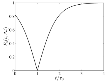
Figure 2: The measurement fidelity $F_{\rm s}(t,\Delta t)$ as a function of the switching time $t$ for $\gamma_{R}/\gamma_{L}=10$ and $\beta=0$. The accuracy to which the switching time is known, $\Delta t$, is assumed to be much smaller than $1/E$. Therefore, the fidelity is independent of $\Delta t$ and is a function of $t$ only. Recall that $\tau_{0}\equiv(\log\gamma_{R}-\log\gamma_{L})/(\gamma_{R}-\gamma_{L})$.

IV.1.2 Overall fidelity

The overall fidelity is now evaluated by taking the statistical average over all possible outcomes

$$F = \sum_{j}F_{j}{\rm Tr}\left\{\hat{U}_{j}\rho_{\rm max.mixed}\hat{U}_{j}^{\dagger}\right\}$$ (57)

$$= \int_{0}^{\infty}F_{\rm s}(t,dt)\frac{P_{\rm s}^{L}(t,t+dt)+P_{\rm s}^{R}(t,t+dt)}{2}$$

$$= \frac{1}{2}\int_{0}^{\infty}\left|\frac{\gamma_{R}e^{-\gamma_{R}t}-\gamma_{L}e^{-\gamma_{L}t}}{\gamma_{R}e^{-\gamma_{R}t}+\gamma_{L}e^{-\gamma_{L}t}}\right|\times$$

$$\hskip 56.9055pt\left(\gamma_{R}e^{-\gamma_{R}t}+\gamma_{L}e^{-\gamma_{L}t}\right)dt$$

$$= \frac{1}{2}\int_{0}^{\tau_{0}}\left(\gamma_{R}e^{-\gamma_{R}t}-\gamma_{L}e^{-\gamma_{L}t}\right)dt+$$

$$\hskip 56.9055pt\frac{1}{2}\int_{\tau_{0}}^{\infty}\left(\gamma_{L}e^{-\gamma_{L}t}-\gamma_{R}e^{-\gamma_{R}t}\right)dt$$

$$= e^{-\gamma_{L}\tau_{0}}-e^{-\gamma_{R}\tau_{0}}$$

$$= \left(\frac{\gamma_{R}}{\gamma_{L}}\right)^{-\frac{\gamma_{L}}{\gamma_{R}-\gamma_{L}}}-\left(\frac{\gamma_{R}}{\gamma_{L}}\right)^{-\frac{\gamma_{R}}{\gamma_{R}-\gamma_{L}}}.$$

This expression for the fidelity is plotted as a function of $\gamma_{R}/\gamma_{L}$ in Fig. 3. One could say that for large values of $\gamma_{R}/\gamma_{L}$ one has a strong measurement, whereas small values of $\gamma_{R}/\gamma_{L}$ correspond to weak measurement. As can be seen from Fig. 2, however, even for small values of $\gamma_{R}/\gamma_{L}$ there can be instances where a high-fidelity outcome is obtained (when $t/\tau_{0}\gg 1$).

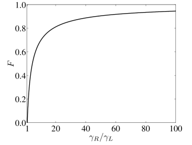
Figure 3: Overall fidelity as a function of the ratio of switching rates $\gamma_{R}/\gamma_{L}$ when the qubit Hamiltonian commutes with the probed qubit operator, i.e. in the special case $\beta=0$.

It is interesting to compare the above result for the overall fidelity with the one that would be obtained in the following situation: Let us assume that we connect the qubit to the detector for some duration $\tau$ and only at the end check whether the detector has switched or not. A switching instance would be associated with the state $\left|R\right\rangle$ and a no-switching instance would be associated with the state $\left|L\right\rangle$. The relevant switching probabilities are given by:

$$P_{\rm s}^{L}(0,\tau) = \left(1-e^{-\gamma_{L}\tau}\right)$$

$$P_{\rm s}^{R}(0,\tau) = \left(1-e^{-\gamma_{R}\tau}\right).$$ (58)

The fidelities for switching and no-switching instances are therefore given by

$$F_{\rm s}(0,\tau) = \frac{e^{-\gamma_{L}\tau}-e^{-\gamma_{R}\tau}}{2-e^{-\gamma_{L}\tau}-e^{-\gamma_{R}\tau}}$$

$$F_{\rm ns}(\tau) = \frac{e^{-\gamma_{L}\tau}-e^{-\gamma_{R}\tau}}{e^{-\gamma_{L}\tau}+e^{-\gamma_{R}\tau}},$$ (59)

and the overall fidelity is given by

$$F = \frac{e^{-\gamma_{L}\tau}-e^{-\gamma_{R}\tau}}{2-e^{-\gamma_{L}\tau}-e^{-\gamma_{R}\tau}}\left(\frac{2-e^{-\gamma_{L}\tau}-e^{-\gamma_{R}\tau}}{2}\right)$$ (60)

$$+\frac{e^{-\gamma_{L}\tau}-e^{-\gamma_{R}\tau}}{e^{-\gamma_{L}\tau}+e^{-\gamma_{R}\tau}}\left(\frac{e^{-\gamma_{L}\tau}+e^{-\gamma_{R}\tau}}{2}\right)$$

$$= e^{-\gamma_{L}\tau}-e^{-\gamma_{R}\tau}.$$

This expression for the overall fidelity is maximized by choosing the pulse duration $\tau=\tau_{0}$ (which was defined in Sec. IV.A.1). This means that the optimal pulse duration is determined by the switching time $\tau_{0}$ at which the fidelity $F_{\rm s}(0,\tau_{0})$ of Eq. (56) vanishes, i.e. the switching time that separates the two time regions associated with the states $\left|L\right\rangle$ and $\left|R\right\rangle$. No enhancement in overall fidelity is obtained by keeping track of the exact switching time.

One thing that can be gained by keeping track of the exact switching time is our knowledge about the state of the qubit after the switching event in a specific experimental run. For example, starting with a maximally mixed state and choosing instances associated with high fidelity (e.g. those with no switching until times much later than $\tau_{0}$), one can predict with a high degree of certainty the qubit’s state after the measurement.

IV.2 Case 2: $E\ll\gamma_{-}$ (Instantaneous measurement)

This case is quite simple as it corresponds to the limit of instantaneous measurement [note that the above condition guarantees that $E\ll\gamma_{R}$; recall that $\gamma_{-}=(\gamma_{R}-\gamma_{L})/2$]. Equations (25) now reduce to

$$\lambda_{\pm} \approx -\frac{\gamma_{+}}{2}\pm\frac{1}{2}\gamma_{-}$$

$$\eta \approx \beta,$$ (61)

such that

$$\hat{U}_{\rm ns}(t) = \hat{U}_{\rm ns}^{\rm meas}(t)$$

$$\hat{U}_{\rm s}(t,\Delta t) = \hat{U}_{\rm s}^{\rm meas}(t,\Delta t)$$

$$\hat{U}_{\rm ns}^{\rm meas}(t) = e^{-\frac{\gamma_{L}}{2}t}\left|L\right\rangle\left\langle L\right|+e^{-\frac{\gamma_{R}}{2}t}\left|R\right\rangle\left\langle R\right|$$

$$\hat{U}_{\rm s}^{\rm meas}(t,\Delta t) = \sqrt{\gamma_{L}\Delta t}\;e^{-\frac{\gamma_{L}}{2}t}\left|L\right\rangle\left\langle L\right|$$ (62)

$$\hskip 14.22636pt+\sqrt{\gamma_{R}\Delta t}\;e^{-\frac{\gamma_{R}}{2}t}\left|R\right\rangle\left\langle R\right|.$$

Note that the energy $E$ does not appear in the above expressions; the detector switches so fast, at least for one of the qubit states, that the measurement is completed before the qubit Hamiltonian contributes any change to the state of the qubit.

The fact that $E$ can be ignored in this case is similar to the situation analyzed in Sec. IV.A (case 1). One can also see that the last two lines in Eq. (62) coincide with Eq. (52). One can therefore follow the analysis of Sec. IV.A [starting from Eq. (52)] in order to calculate the measurement fidelity for the instantaneous-measurement case under the different possible scenarios. Not surprisingly, the measurement basis is $\{\left|L\right\rangle,\left|R\right\rangle\}$, which is natural given the fact that the measurement is instantaneous, and the measurement basis should coincide with the natural measurement basis of the detector.

As in Sec. IV.A, the overall fidelity is given by Eq. (57) [which is plotted in Fig. 3]. In the limit $\gamma_{R}/\gamma_{L}\rightarrow\infty$, the fidelity is one, and one obtains the simple case of a strong (projective) measurement in the basis $\left\{\left|L\right\rangle,\left|R\right\rangle\right\}$. Note that the limit $\gamma_{R}/\gamma_{L}\rightarrow 0$ gives the same result, with the roles of $\gamma_{L}$ and $\gamma_{R}$ reversed.

In the limit $\gamma_{-}\ll\gamma_{+}$ (i.e. when $\gamma_{R}/\gamma_{L}$ is close to one), we still have an instantaneous measurement, but with a low fidelity. The measurement in this limit is therefore a weak measurement. The switching time of the detector allows the experimenter to make a guess about the state of the qubit, but with a small degree of confidence. Repeated measurements of this type, possibly synchronized with the qubit’s free precession, on a single qubit would increase the acquired amount of information (or degree of certainty) about the state of the qubit, thus approaching the case of a strong measurement.

IV.3 Case 3: $E\gg\gamma_{+}$ (Slow measurement)

The opposite limit of case 2 is the one with $E\gg\gamma_{-}$. However, when $\gamma_{-}\ll E\ll\gamma_{+}$, we recover the case of an instantaneous, weak measurement (with minor changes). Therefore, in this subsection we focus on the case where $E$ is larger than both $\gamma_{-}$ and $\gamma_{+}$.

When $E\gg\gamma_{-}$, we find that (see Appendix A)

$$\hat{U}_{\rm ns}^{\dagger}(t)\hat{U}_{\rm ns}(t) = \left(\begin{array}[]{cc}e^{-(\gamma_{+}-\gamma_{-}\cos\beta)t}&0\\ 0&e^{-(\gamma_{+}+\gamma_{-}\cos\beta)t}\end{array}\right)$$ (65)

$$\hat{U}_{\rm s}^{\dagger}(t,\Delta t)\hat{U}_{\rm s}(t,\Delta t) = P_{\rm s}^{(1)}(t,\Delta t)\left|\psi_{\rm s}^{(1)}(t)\right\rangle\left\langle\psi_{\rm s}^{(1)}(t)\right|+P_{\rm s}^{(2)}(t,\Delta t)\left|\psi_{\rm s}^{(2)}(t)\right\rangle\left\langle\psi_{\rm s}^{(2)}(t)\right|$$ (66)

where

$$\left|\psi_{\rm s}^{(1)}(t)\right\rangle = \left(\begin{array}[]{c}\cos\frac{\theta(t)}{2}e^{-i\frac{\tilde{E}}{2}t}\\ \sin\frac{\theta(t)}{2}e^{i\frac{\tilde{E}}{2}t}\\ \end{array}\right)=\left(\begin{array}[]{cc}e^{-i\frac{\tilde{E}}{2}t}&0\\ 0&e^{i\frac{\tilde{E}}{2}t}\\ \end{array}\right)\left(\begin{array}[]{c}\cos\frac{\theta(t)}{2}\\ \sin\frac{\theta(t)}{2}\\ \end{array}\right)$$ (73)

$$\left|\psi_{\rm s}^{(2)}(t)\right\rangle = \left(\begin{array}[]{c}\sin\frac{\theta(t)}{2}e^{-i\frac{\tilde{E}}{2}t}\\ -\cos\frac{\theta(t)}{2}e^{i\frac{\tilde{E}}{2}t}\\ \end{array}\right)=\left(\begin{array}[]{cc}e^{-i\frac{\tilde{E}}{2}t}&0\\ 0&e^{i\frac{\tilde{E}}{2}t}\\ \end{array}\right)\left(\begin{array}[]{c}\sin\frac{\theta(t)}{2}\\ -\cos\frac{\theta(t)}{2}\\ \end{array}\right)$$ (80)

$$\tilde{E} = E-\gamma_{-}^{2}/2E$$

$$\tan\theta(t) = \frac{(\gamma_{L}-\gamma_{R})\sin\beta}{\gamma_{L}\left(e^{\gamma_{-}t\cos\beta}\cos^{2}\frac{\beta}{2}-e^{-\gamma_{-}t\cos\beta}\sin^{2}\frac{\beta}{2}\right)+\gamma_{R}\left(e^{\gamma_{-}t\cos\beta}\sin^{2}\frac{\beta}{2}-e^{-\gamma_{-}t\cos\beta}\cos^{2}\frac{\beta}{2}\right)}$$

$$P_{\rm s}^{(1)}(t,\Delta t)+P_{\rm s}^{(2)}(t,\Delta t) = e^{-\gamma_{+}t}\Delta t$$

$$\left\{\gamma_{L}\left(e^{\gamma_{-}t\cos\beta}\cos^{2}\frac{\beta}{2}+e^{-\gamma_{-}t\cos\beta}\sin^{2}\frac{\beta}{2}\right)+\gamma_{R}\left(e^{\gamma_{-}t\cos\beta}\sin^{2}\frac{\beta}{2}+e^{-\gamma_{-}t\cos\beta}\cos^{2}\frac{\beta}{2}\right)\right\}$$

$$P_{\rm s}^{(1)}(t,\Delta t)-P_{\rm s}^{(2)}(t,\Delta t) = e^{-\gamma_{+}t}\Delta t\frac{(\gamma_{L}-\gamma_{R})\sin\beta}{\sin\theta(t)}.$$ (81)

Recall that, in spite of their appearance, the operators $\hat{U}_{\rm ns}(t)$ and $\hat{U}_{\rm s}(t,\Delta t)$ are not unitary matrices.

For short times ($t=0$), the above expressions reduce to

$$\theta = \beta$$

$$P_{\rm s}^{(1)}+P_{\rm s}^{(2)} = \Delta t\left(\gamma_{L}+\gamma_{R}\right)$$

$$P_{\rm s}^{(1)}-P_{\rm s}^{(2)} = \Delta t(\gamma_{L}-\gamma_{R})$$

$$F_{\rm s}(0,\Delta t) = \frac{\gamma_{R}-\gamma_{L}}{\gamma_{R}+\gamma_{L}},$$ (82)

such that the measurement basis coincides with the detector’s natural measurement basis, as it should for short times (where the qubit Hamiltonian has not affected the qubit’s state). For long times ($\gamma_{-}t\rightarrow\infty$) [and $\beta\neq\pi/2$], on the other hand, the above expressions reduce to

$$\theta \rightarrow 0$$

$$P_{\rm s}^{(1)}+P_{\rm s}^{(2)} = e^{-\gamma_{+}t}\Delta t\left\{\gamma_{L}e^{\gamma_{-}t\cos\beta}\cos^{2}\frac{\beta}{2}+\gamma_{R}e^{\gamma_{-}t\cos\beta}\sin^{2}\frac{\beta}{2}\right\}$$

$$P_{\rm s}^{(1)}-P_{\rm s}^{(2)} = e^{-\gamma_{+}t}\Delta t\left\{\gamma_{L}e^{\gamma_{-}t\cos\beta}\cos^{2}\frac{\beta}{2}+\gamma_{R}e^{\gamma_{-}t\cos\beta}\sin^{2}\frac{\beta}{2}\right\}$$

$$F(t\rightarrow\infty,\Delta t) = 1,$$ (83)

such that the measurement is performed in the qubit’s energy eigenbasis with 100% fidelity. Thus the measurement basis starts from the detector’s natural measurement basis (i.e. $\left\{\left|L\right\rangle,\left|R\right\rangle\right\}$) at $t=0$ and spirals towards the $z$ axis (i.e. $\left\{\left|0\right\rangle,\left|1\right\rangle\right\}$) with time. Note that since the denominator in the first line of Eq. (81) goes from negative values (e.g. at $t=0$) to positive values (e.g. when $t\rightarrow\infty$) the measurement basis goes through the equator during its spiraling motion.

From the above results, we can see that the measurement is made in a rotated basis that is determined by the exact switching time, which is uncontrollable. Each experimental run gives a measurement outcome that is different from other identically prepared runs. Note, in particular, that when $\gamma_{L}=0$ the fidelity is 100% for all switching times $t$ (which can be verified with straightforward algebra). This result is quite interesting; even though the fidelity is 100% for every single run, the measurement basis is unpredictable and is only determined when the switching event occurs.

Let us now consider the situation where we know only whether the detector switched between $t=0$ and $t=\tau$ (with $\tilde{E}\tau\gg 1$) or not. The measurement matrices that correspond to these two possible outcomes are given by

$$\hat{U}_{\rm s}^{\dagger}(0,\tau)\hat{U}_{\rm s}(0,\tau) = \int_{0}^{\tau}\hat{U}_{\rm s}^{\dagger}(t,dt)\hat{U}_{\rm s}(t,dt)$$ (84)

$$= 1-\hat{U}_{\rm ns}^{\dagger}(\tau)\hat{U}_{\rm ns}(\tau),$$

and $\hat{U}_{\rm ns}^{\dagger}(\tau)\hat{U}_{\rm ns}(\tau)$ as given in Eq. (66). Since the measurement matrices are diagonal in the qubit’s energy eigenbasis, the measurement is performed in that basis. The overall fidelity can be calculated similarly to what was done in Sec. IV.A:

$$F=e^{-(\gamma_{+}-\gamma_{-}\cos\beta)\tau}-e^{-(\gamma_{+}+\gamma_{-}\cos\beta)\tau}.$$ (85)

This expression is maximized by choosing

$$\tau=\frac{\log\frac{\gamma_{+}+\gamma_{-}\cos\beta}{\gamma_{+}-\gamma_{-}\cos\beta}}{2\gamma_{-}\cos\beta},$$ (86)

which gives the maximum fidelity

$$F_{\rm max} = \left(\frac{\gamma_{+}-\gamma_{-}\cos\beta}{\gamma_{+}+\gamma_{-}\cos\beta}\right)^{\frac{\gamma_{+}-\gamma_{-}\cos\beta}{2\gamma_{-}\cos\beta}}$$ (87)

$$\hskip 28.45274pt-\left(\frac{\gamma_{+}-\gamma_{-}\cos\beta}{\gamma_{+}+\gamma_{-}\cos\beta}\right)^{\frac{\gamma_{+}+\gamma_{-}\cos\beta}{2\gamma_{-}\cos\beta}}.$$

Since the above expression looks somewhat cumbersome, we shall not pursue it in its general form any further. In the special case $\gamma_{L}=0$, the overall fidelity for a readout pulse of duration $\tau$ is given by

$$F=e^{-\gamma_{R}\tau\sin^{2}\frac{\beta}{2}}-e^{-\gamma_{R}\tau\cos^{2}\frac{\beta}{2}},$$ (88)

which is maximized by choosing

$$\tau=\frac{-\log\tan^{2}\frac{\beta}{2}}{\gamma_{R}\cos\beta}.$$ (89)

The maximum fidelity is therefore given by

$$F_{\rm max} = \left(\tan\frac{\beta}{2}\right)^{\frac{2\sin^{2}(\beta/2)}{\cos\beta}}-\left(\tan\frac{\beta}{2}\right)^{\frac{2\cos^{2}(\beta/2)}{\cos\beta}}$$ (90)

$$= \left(\tan\frac{\beta}{2}\right)^{\sec\beta-1}-\left(\tan\frac{\beta}{2}\right)^{\sec\beta+1}.$$

This expression is plotted in Fig. 4. The measurement fidelity decreases as $\beta$ approaches $\pi/2$ and vanishes at that point.

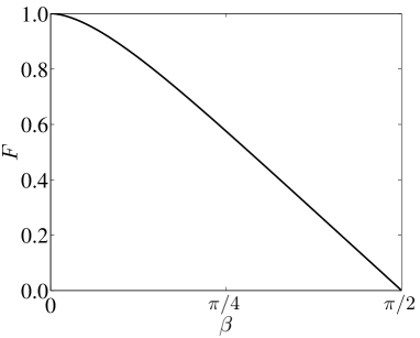
Figure 4: Maximum fidelity as a function of the angle between the qubit Hamiltonian and measurement axes, assuming that the exact switching time is not known (up to the measurement duration, which is taken to be much larger than $1/E$).

For further demonstration of the results discussed in this section, see Appendix B, where the special case $\beta=\pi/2$ is analyzed in some detail.

IV.4 All-in-one measurement setting

Looking at the results of Sec. IV.C (case 3), it is interesting that every time the experiment is repeated, the measurement outcome gives information about the qubit state in a different basis (that cannot be predicted beforehand). This result suggests that it could be possible to perform ‘single-setting quantum state tomography’ Single_setting ; instead of the externally applied rotations used to perform measurements in different bases in conventional quantum state tomography, the (uncontrollable) switching times determine the measurement basis in each experimental run. Indeed, using Eq. (136) we find that the switching probability as a function of time is given by

$${\rm Prob_{s}}(t,\Delta t) = {\rm Tr}\left\{\hat{U}_{\rm s}^{\dagger}(t,\Delta t)\hat{U}_{\rm s}(t,\Delta t)\rho(0)\right\}$$ (91)

$$= e^{-\gamma_{+}t}\Delta t\Bigg{[}\rho_{00}e^{\gamma_{-}t\cos\beta}\left(\gamma_{+}-\gamma_{-}\cos\beta\right)$$

$$+\rho_{11}e^{-\gamma_{-}t\cos\beta}\left(\gamma_{+}+\gamma_{-}\cos\beta\right)$$

$$-\left(\rho_{10}+\rho_{01}\right)\frac{\gamma_{-}}{4}\sin\beta\cos\tilde{E}t$$

$$-\left(\frac{\rho_{10}-\rho_{01}}{i}\right)\frac{\gamma_{-}}{4}\sin\beta\sin\tilde{E}t\Bigg{]}.$$

By fitting the experimentally measurable switching-time probability distribution to the above function, one can extract the three quantities $\left(\rho_{11}-\rho_{00}\right)$, $\left(\rho_{10}+\rho_{01}\right)$ and $\left(\rho_{10}-\rho_{01}\right)/i$, which completely characterize the quantum state of the qubit. In addition to the above three parameters, one can also extract the values of $\gamma_{L}$, $\gamma_{R}$, $\beta$ and $E$, thus providing an all-in-one measurement that characterizes both the system parameters as well as the quantum state of the qubit Aharonov . Note that in the special cases $\beta=0$, $\beta=\pi/2$ and $\gamma_{+}\gg E$ full system characterization and state tomography are not possible, in agreement with intuitive expectations. In particular, the case $\beta=0$ corresponds to a measurement in the $\{\left|0\right\rangle,\left|1\right\rangle\}$ basis (regardless of the switching time), which clearly cannot give any information about the quantities $\left(\rho_{10}+\rho_{01}\right)$ and $\left(\rho_{10}-\rho_{01}\right)/i$.

V Coherent detector

In the preceding two sections, we have focused on the regime where the coherence time between the two detector states (i.e. the switched and non-switched states $\left|S\right\rangle$ and $\left|N\right\rangle$) is the shortest timescale in the problem. Now we turn to the case where this time is longer than $1/E$, which now is the shortest timescale in the problem.

We should emphasize here the distinction between this case of a coherent detector and the case of a ‘slow’ but incoherent detector (with a small switching rate; $\gamma_{+}\ll E$) analyzed in the previous section Martin . That situation was analyzed using the same theoretical framework as any other case with an incoherent detector. We should also emphasize that, in spite of the detector’s long coherence time (compared to $1/E$), we still assume irreversible switching. These assumptions are compatible; for irreversibility one only needs to assume that the detector’s coherence time is much shorter than the inverse of the switching rate. The assumptions explained above can be summarized as follows:

$$\frac{1}{E}\ll{\rm coh.\ time\ of\ detector}\ll\frac{1}{\rm switching\ rate}.$$ (92)

Since we are now treating the detector as a quantum-coherent object (at least on the timescale of qubit precession), we analyze the dynamics using a Hamiltonian that describes the combined qubit-detector system. Since the Hamiltonian contains the physical interaction between the qubit and the detector, in this section we find it easier to define the qubit’s $z$ axis as defined by the probed operator. Thus, the Hamiltonian can be expressed as

$$\hat{H}=\hat{H}_{\rm q}+\hat{H}_{\rm det},$$ (93)

where

$$\hat{H}_{\rm q} = -\frac{E}{2}\left(\sin\beta\hat{\sigma}_{x}+\cos\beta\hat{\sigma}_{z}\right)$$

$$\hat{H}_{\rm det} = \left\{g_{L}\left(\left|S\right\rangle\left\langle N\right|+h.c.\right)+\epsilon_{L}\left|S\right\rangle\left\langle S\right|\right\}\left|L\right\rangle\left\langle L\right|+$$ (94)

$$\left\{g_{R}\left(\left|S\right\rangle\left\langle N\right|+h.c.\right)+\epsilon_{R}\left|S\right\rangle\left\langle S\right|\right\}\left|R\right\rangle\left\langle R\right|,$$

$g_{L}$ and $g_{R}$ are the coupling strengths that induce detector switching for the qubit states $|L\rangle$ and $|R\rangle$, respectively, and $\epsilon_{L}$ and $\epsilon_{R}$ are relative energy biases between the states $\left|N\right\rangle$ and $\left|S\right\rangle$ for the two qubit states. As before, the detector is assumed to be initially in the state $\left|N\right\rangle$.

Since the qubit’s energy is the largest energy scale in the problem, the dynamics described by the above Hamiltonian and the detector’s decoherence cannot induce transitions between the qubit’s ground and excited states (note also that we are ignoring any intrinsic decoherence mechanisms of the qubit). We can therefore analyze the dynamics by treating two separate subspaces of the Hilbert space, one with the qubit in the ground state $\left|0\right\rangle$ and one with the qubit in the excited state $\left|1\right\rangle$. This approach results in two effective Hamiltonians for the detector:

$$\hat{H}_{{\rm det},\left|0\right\rangle} = {}_{\rm qubit}\left\langle 0\right|\hat{H}\left|0\right\rangle_{\rm qubit}$$

$$= \bar{g}_{0}\left(\left|S\right\rangle\left\langle N\right|+h.c.\right)+\bar{\epsilon}_{0}\left|S\right\rangle\left\langle S\right|$$

$$\hat{H}_{{\rm det},\left|1\right\rangle} = {}_{\rm qubit}\left\langle 1\right|\hat{H}\left|1\right\rangle_{\rm qubit}$$ (95)

$$= \bar{g}_{1}\left(\left|S\right\rangle\left\langle N\right|+h.c.\right)+\bar{\epsilon}_{1}\left|S\right\rangle\left\langle S\right|,$$

where

$$\bar{g}_{0} = g_{L}\cos^{2}\frac{\beta}{2}+g_{R}\sin^{2}\frac{\beta}{2}$$

$$\bar{g}_{1} = g_{L}\sin^{2}\frac{\beta}{2}+g_{R}\cos^{2}\frac{\beta}{2}$$

$$\bar{\epsilon}_{0} = \epsilon_{L}\cos^{2}\frac{\beta}{2}+\epsilon_{R}\sin^{2}\frac{\beta}{2}$$

$$\bar{\epsilon}_{1} = \epsilon_{L}\sin^{2}\frac{\beta}{2}+\epsilon_{R}\cos^{2}\frac{\beta}{2}.$$ (96)

In order to avoid running into complicated expressions below, we make the experimentally relevant assumption that the switching for the state $\left|R\right\rangle$ is much faster than that for the state $\left|L\right\rangle$. This situation occurs when one or both of the following conditions are satisfied: (1) $|g_{R}|\gg|g_{L}|$ or (2) $|\epsilon_{L}|$ is much larger than all other parameters relevant to the switching dynamics. We analyze these two cases separately.

First we consider the case where $|g_{R}|\gg|g_{L}|$, such that $g_{L}$ can be ignored in the following analysis. For simplicity and clarity, we take $\epsilon_{L}$ and $\epsilon_{R}$ to be smaller than the detector’s coherence time, such that they also can be ignored for purposes of this calculation. Equations (95) therefore reduce to

$$\hat{H}_{{\rm det},\left|0\right\rangle} = g_{R}\sin^{2}\frac{\beta}{2}\left(\left|S\right\rangle\left\langle N\right|+h.c.\right)$$

$$\hat{H}_{{\rm det},\left|1\right\rangle} = g_{R}\cos^{2}\frac{\beta}{2}\left(\left|S\right\rangle\left\langle N\right|+h.c.\right).$$ (97)

Since we are assuming that the switching is an incoherent process (or, in other words, the detector’s coherence time is much shorter than $|g_{R}|$), the switching rates are proportional to the squares of the transition coefficients in the above Hamiltonians. The switching rates for the qubit states $\left|0\right\rangle$ and $\left|1\right\rangle$ can therefore be expressed as

$$\Gamma_{0} = \Gamma_{R}\sin^{4}\frac{\beta}{2}$$

$$\Gamma_{1} = \Gamma_{R}\cos^{4}\frac{\beta}{2}.$$ (98)

We now consider the second case, where $|\epsilon_{L}|$ is very large compared to all other parameters relevant to the switching dynamics. In this case the switching rates are governed by the scaling formula

$$\Gamma_{j}\propto\frac{\bar{g}_{j}^{2}}{|\bar{\epsilon}_{j}|}.$$ (99)

With the simplifying assumption that $g_{L}=g_{R}$, we find switching rates of the form

$$\Gamma_{0} = \Gamma_{R}\sec^{2}\frac{\beta}{2}$$

$$\Gamma_{1} = \Gamma_{R}\csc^{2}\frac{\beta}{2}.$$ (100)

Note that the divergence of $\Gamma_{1}$ for $\beta\rightarrow 0$ is an artefact of our approximations. In a more accurate description, $\Gamma_{1}$ would saturate at a finite value as $\beta$ approaches zero.

The difference between the expressions in Eqs. (98) and (100) shows that, in the case of a coherent detector, knowledge of the microscopic details of the detector is necessary in order to determine the dependence of the switching rates on the angle $\beta$. On the other hand, this sensitivity to details could be useful for experimentally testing theoretical models of the detector.

One common, and important, result for the different cases with a coherent detector, however, can be seen by noting that the qubit’s state in the energy eigenbasis $\left\{\left|0\right\rangle,\left|1\right\rangle\right\}$ does not change during the measurement. Therefore, the detector cannot be performing a measurement on the qubit in any basis other than this one. Since, in addition, the detector’s switching rate depends on the qubit’s state in the energy eigenbasis, one can conclude that the detector does in fact perform a measurement on the qubit in the energy eigenbasis. Using the transition rates given in Eq. (98) or (100), one can follow the analysis of Sec. IV.A and determine the fidelity of the measurement setup. The two expressions found in this section describe a fidelity that slowly decreases from unity at $\beta=0$ to zero at $\beta=\pi/2$. This result seems to be unavoidable for the two-state-detector model considered so far. In spite of the different functional dependence, the fidelity decrease is somewhat similar to the one obtained in Sec. IV.C for an incoherent detector with small switching rates [see Eq. (90)]. In Sec. VII, we shall discuss a system where the fidelity of a coherent detector remains very close to unity even as $\beta$ approaches $\pi/2$.

VI Comparison between different types of detectors

To conclude the above analysis of the detector’s operation, we present in Table I the measurement basis and the factors limiting the measurement fidelity in different operation regimes.

Detector type	Measurement	Meas. fidelity
	basis	limited by
Fast switching	$\left\{\left|L\right\rangle,\left|R\right\rangle\right\}$	$\gamma_{R}/\gamma_{L}$
Slow switching,	determined	$\gamma_{R}/\gamma_{L}$
incoherent, switching time	upon switching
accurately measurable
Slow switching,	$\left\{\left|0\right\rangle,\left|1\right\rangle\right\}$	$\gamma_{R}/\gamma_{L}$ and $\beta$
incoherent, exact switching
time inaccessible
Slow switching,	$\left\{\left|0\right\rangle,\left|1\right\rangle\right\}$	$\gamma_{R}/\gamma_{L}$ and $\beta$
coherent		(in two-state
		model; Sec. V)

Table I: Measurement basis and fidelity for different types of detectors characterized by their coupling strength to the qubit, their coherence times and whether the switching time can be known accurately or not. In the case of a weakly coupled coherent detector, we give the results for the two-state-detector model only.

It is worth mentioning here a distinction between two different types of weak measurement, i.e. a measurement with low fidelity. There are cases where the interaction between the qubit and the detector is such that it is fundamentally impossible for any observer (with full access to all degrees of freedom of the detector) to determine with certainty the state of the qubit. The situations analyzed in Secs. IV.A, IV.B and V correspond to this type of weak measurement. In this case, there is no lost information, and an initially pure state of the qubit remains pure after the measurement (note that not knowing the exact switching time to an accuracy $\Delta t$ that is much smaller than $1/E$ does not constitute lost, and relevant, information in this context; Going to higher accuracies within the regime $E\Delta t\ll 1$ provides more information about the state of the detector, but not that of the qubit). The situation where the observer cannot establish the exact switching time of an incoherent detector to an accuracy smaller than $1/E$ (analyzed in Sec. IV.C) involves information that is collected by the detector and potentially measurable, but inaccessible to the observer in the experimental situation under consideration. In this case, the qubit’s state after the measurement is generally a mixed state (obtained by averaging over all possible outcomes within the experimenter’s accuracy range), even if the initial state is pure. One could say that the accessible information serves as measurement data, whereas information that is collected by the detector but is inaccessible to the experimenter plays the role of a decoherence mechanism.

We now pause for a moment to comment on the issue of qubit decoherence. In some experimental situations, the detector enhances the qubit’s decoherence rate Makhlin . This additional decoherence channel typically causes loss of coherence in the $\{\left|L\right\rangle,\left|R\right\rangle\}$ basis. If the decoherence rate is larger than the qubit’s energy scale $E$, the qubit’s state will be frozen in the $\{\left|L\right\rangle,\left|R\right\rangle\}$ basis during the measurement. In that case, the detector’s operation resembles that in the instantaneous (and possibly strong-measurement) regime, even if the switching rates are small compared to $E$. Thus, such an additional decoherence could be detected by analyzing the operation of the detector and comparing it with the expected behaviour in the absence of decoherence Picot . It is also worth mentioning here that including decoherence into our theoretical analysis would be quite nontrivial. The evolution of the qubit’s state during the short interval $\delta t$ would have to be described by the sum of terms, and not just a single propagator as was the case in our analysis. It would therefore not be possible to derive a simple analytic expression for the matrix $\hat{U}_{\rm ns}(t)$ in the presence of decoherence as we were able to do in Eq. (24).

To conclude the discussion of the two-state model, we summarize some of the main principles that have been demonstrated in the above analysis. For a strong measurement, the detector always measured the qubit in the $\{\left|L\right\rangle,\left|R\right\rangle\}$ basis. In the case of a slow, incoherent detector whose switching time can be determined accurately, one could say that, to a lowest approximation, the qubit’s state precesses freely following the qubit Hamiltonian and is then measured in the $\{\left|L\right\rangle,\left|R\right\rangle\}$ basis when the detector switches. When the switching time can only be known with small accuracy (i.e. much longer than the qubit’s precession period), the detector effectively probes the qubit in the energy eigenbasis, with the corresponding switching rates being obtained as weighted averages of the bare switching rates $\gamma_{L}$ and $\gamma_{R}$. A slow, coherent detector measures the qubit in the energy eigenbasis, with the detector effectively following weighted-average Hamiltonians for the two energy eigenstates.

VII Application to superconducting flux qubits

In the preceding sections we have analyzed a theoretical model where the detector is a two-state system. We now turn to a specific physical example of switching-based measurement, namely the readout of a superconducting flux qubit OtherQubitTypes . Although the two-state-detector model does not provide an accurate description of the complex circuits that we discuss in this section, the insight developed in the preceding sections (in particular the general principles summarized in Sec. VI) will allow us to infer a number of results concerning the realistic situations that we consider here.

There are two qubit-readout methods used in experiment that rely on a switching process in a superconducting circuit: switching from a zero-voltage to a finite-voltage state across a dc superconducting quantum interference device (SQUID) VanderWal and switching between two possible dynamical states of a nonlinear oscillator Siddiqi (For a theoretical study on measurement in superconducting qubits, see e.g. Johansson ; and for studies on quantum tunneling between dynamical states in superconducting systems, see e.g. Marthaler ; Serban ; Nation ). Both of the readout methods mentioned above can be modelled theoretically as a fictitious particle moving in a trapping potential. Therefore, their behaviour in terms of switching dynamics should exhibit the same features, which we discuss below.

We briefly explain the operation of the dc-SQUID detector that relies on switching from the zero-voltage state to the finite-voltage state of a current biased dc-SQUID (see also Nakano ; MaassenVDB ); as mentioned above, the analysis of the dynamical bifurcation would be similar. The principle of the measurement process is as follows: The dc-SQUID is known to be a highly sensitive device for measuring magnetic fields. In the presence of an externally applied magnetic flux and a bias current that is close to a certain (critical) value, the switching rate of the dc-SQUID from the zero-voltage to the finite-voltage state varies greatly with even small changes in magnetic field. When a flux qubit is placed next to a dc-SQUID biased close to the switching point, the clockwise- and counterclockwise-current states of the qubit can result in two switching rates that are different by orders of magnitude. By choosing suitable values for the applied bias current and the length of the current pulse, the SQUID switches with high probability for one qubit state and with low probability for the other qubit state. The contrast between the two switching probabilities is perhaps most clearly visualized in the so-called S curves. These curves are produced by plotting the SQUID’s switching probability as a function of bias current for the qubit’s clockwise- and counterclockwise-current states (for a fixed measurement duration). An example of such S curves is shown in Fig. 5 (dashed lines).

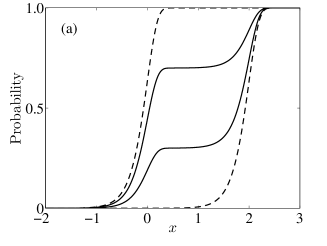
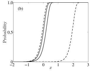
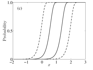
Figure 5: The S curves (i.e. switching probabilities as functions of readout bias current with fixed pulse duration) for three different types of detectors: a strongly coupled detector [(a); see Sec. IV.B], a weakly coupled fast-decohering detector [(b); see Sec. IV.C] and a weakly coupled slow-decohering detector [(c); see Sec.V]. The dashed lines are the S curves for the qubit’s clockwise- and counterclockwise-current states, i.e. the ones that are obtained when the qubit is biased far from the degeneracy point. In the example plotted in this figure, the probabilities for these S curves (i.e. the dashed lines) are given by $P=1-e^{-\gamma_{L/R}t}$ with $\gamma_{L}t=e^{5(x-2)}$ and $\gamma_{R}t=e^{5x}$ ($x$ is a dimensionless parameter that represents the bias current used in the readout pulse, and $\gamma_{L/R}$ represent the switching rates for the two different persistent-current states). The solid lines are the S curves for the qubit’s energy eigenstates when these states have the form $\left|0\right\rangle=\sqrt{0.7}\left|L\right\rangle+\sqrt{0.3}\left|R\right\rangle$ and $\left|1\right\rangle=\sqrt{0.3}\left|L\right\rangle-\sqrt{0.7}\left|R\right\rangle$. In (a) the switching probabilities for the states $\left|L\right\rangle$ and $\left|R\right\rangle$ are averaged (in a weighted manner) in order to obtain the switching probabilities for the states $\left|0\right\rangle$ and $\left|1\right\rangle$. This reasoning is the one that would be consistent with the picture of a strong measurement. In (b) the switching rates are averaged, and the switching probabilities are calculated from the averaged switching rates (see Sec. IV.C). In (c) the parameter $x$ is averaged, and from the two weighted averages of $x$ the switching rates and probabilities are calculated (see Sec. V). Here we are treating $x$ as the physical observable that is modified by the qubit at the Hamiltonian level.

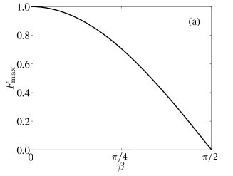
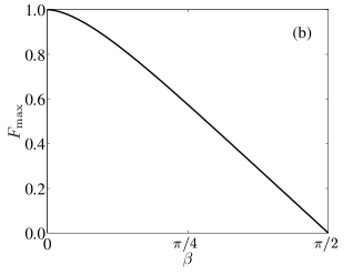
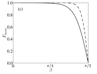
Figure 6: The maximum measurement fidelity (i.e. at the optimal value of $x$) as a function of the angle $\beta$ (between the qubit Hamiltonian’s axis and the probed operator axis) for the three different types of detectors whose S curves are plotted in Fig. 5. The fidelity is derived by finding the maximum vertical separation between the two S-curves for a given value of $\beta$. In (a) the fidelity is given by $\cos\beta$, as expected for the textbook-type projective measurement. In (b) the fidelity is given by Eq. (90). In (c) the fidelity is calculated numerically. For further demonstration that the coherent detector’s fidelity can remain close to 100% even for $\beta\neq 0$, we plot in Fig. 6c (dashed line) the fidelity when the coefficient 5 in the switching-rate formulae of Fig. 5 is replaced by the coefficient 10 (i.e. in going from the solid to the dashed line, the sensitivity of the detector is increased).

We now ask the question of what the S curves would look like if the qubit were biased close to the so-called degeneracy point, where the energy eigenstates are superpositions of the two persistent-current eigenstates. Figure 5 shows three possibilities that correspond to three different types of detectors: a strongly coupled detector (see Sec. IV.B), a weakly coupled fast-decohering detector (see Sec. IV.C) and a weakly coupled slow-decohering detector (see Sec.V) [the explanation of the reasoning behind each one the obtained shapes of the S-curves is given in Sec. VI]. In Fig. 6 we plot the measurement fidelity (at the optimal bias current) for the three different types of detectors. Clearly, these three types of detectors operate drastically differently. The fidelity in Fig. 6(a) is given by $\cos\beta$, and the one in Fig. 6(b) is given by Eq. (90), i.e. it is identical to the one shown in Fig. 4. As mentioned above (see also Ashhab ), the measurement fidelity of a coherent detector (Fig. 6c) can remain close to 100% even when the qubit Hamiltonian and the probed operator do not commute.

The operation of the detector when the qubit is biased close to the degeneracy point can be used to identify whether it performs a strong- or weak-coupling measurement and how the detector’s coherence time compares to the qubit’s precession period. By tuning the qubit’s energy splitting and probing it using the detector, it could be possible to measure the coherence time of the detector. This approach could also be used to probe coherent behaviour in the detector.

Finally, we comment on the description of a continuous-variable switching detector, which should be a good description for the dc-SQUID-based measurement of the flux qubit (see also Nakano ). Instead of our two-state-detector model, one can in general use a model of a fictitious particle initialized in a local minimum of a one-dimensional potential. The clockwise- and counterclockwise-current states of the qubit correspond to slightly different potentials for this particle. The two potentials can result in very different escape rates (out of the local minimum). We expect that in the case of an incoherent detector the above results for a two-state detector also hold for the continuous-variable detector. In the case of a coherent detector, one can follow the general procedure that we used for the two-state detector, modified for the continuous-variable detector. One takes the two trapping potentials for the clockwise- and counterclockwise-current states. From these potentials one derives two effective potentials (that correspond to the qubit’s two energy eigenstates) for the fictitious particle, each potential obtained as a weighted average of the two bare potentials. The proper proportions of the original potentials that are used to evaluate the energy-eigenstate effective potentials are determined by the mixing probabilities of the persistent-current states in the energy eigenstates. These weighted-average potentials now determine the relevant escape rates for the particle, and these escape rates characterize the operation of the detector. As in Sec. V (two-state coherent detector), the detector performs a measurement on the qubit in the energy eigenbasis. However, as can be seen in Fig. 6(c), the continuous-variable detector has the advantage that it could lead to a high fidelity measurement even when the energy eigenstates are superpositions of persistent-current states. In fact, such high-fidelity readout in the energy eigenbasis was observed in the experiment of Ref. Tanaka .

A note is in order here on the relevant coherence time that separates the coherent-detector and incoherent-detector regimes for a continuous-variable detector. Even if the coherence time between the switched (or escaped) state and the non-switched (or trapped) state is short, the coherence time that corresponds to motion around the local minimum of the trapping potential could still be long. If (1) the temperature is low enough such that the detector’s fictitious particle is almost in the ground state of its effective potential and (2) the coherence time for superpositions of the ground states of the two possible effective potentials is longer than $1/E$, the detector would operate in the coherent regime [Fig. 6(c)]. A full understanding of the boundary at which decoherence in the detector causes irreversible collapse of the state of the system and how that affects the state of the qubit is lacking. Our results demonstrate that the coherence properties of the detector are crucial for determining its regime of operation. However, they do not answer questions about the coherence within the trapped state, or states, of the detector.

VIII Conclusion

We have analyzed the operation of a switching-based detector that is used to measure the state of a qubit in the case when the probed observable does not commute with the qubit Hamiltonian. We have found several operation regimes depending on the relation between the detector’s switching rate and the qubit’s energy (strong versus weak-coupling measurement) and the relation between the detector’s coherence time and the qubit’s energy (coherent versus incoherent detector). The accessibility of the exact switching time also plays a role in determining the performed measurement. Table I summarizes the differences between the different regimes.

The weak-coupling regimes result in a number of interesting phenomena. For example, an incoherent detector can be used for an ‘all-in-one’ measurement setting that can be used to simultaneously calibrate the system and perform quantum-state tomography. Apart from isolated special cases, a coherent detector always measures the qubit in its energy eigenbasis, regardless of the quantity that it naturally probes. Furthermore, the measurement fidelity of a coherent detector can remain close to 100%, even when the qubit’s Hamiltonian and the qubit operator being probed by the detector do not commute.

Although we have analyzed a simplified two-state-detector model that was inspired by the measurement of superconducting flux qubits using dc SQUIDs, the main results should apply to other types of qubits and measurement devices, e.g. charge qubits measured using a quantum point contact Gurvitz . As far as the roles of the different coherence and coupling parameters are concerned, our results provide insight into the operation of a general type of detector and can be useful for future studies aimed at designing high-fidelity measurement devices.

We would like to thank P. de Groot, C. Harmans, K. Harrabi, A. Kofman, A. J. Leggett, Y. Nazarov, T. Picot and H. Wei for useful discussions, and especially P. Bertet for drawing our attention to the significance of the S-curves as a diagnostic tool for characterizing the detector’s operation. This work was supported in part by the National Security Agency (NSA), the Laboratory for Physical Sciences (LPS), the Army Research Office (ARO) and the National Science Foundation (NSF) grant No. EIA-0130383. J.Q.Y. was also supported by the National Basic Research Program of China grant No. 2009CB929300, the National Natural Science Foundation of China grant No. 10625416, and the MOST International Collaboration Program grant No. 2008DFA01930.

Appendix A:
Incoherent detector with $E\gg\gamma_{-}$

When $E\gg\gamma_{-}$, Eq. (25) gives

$$\lambda_{\pm} \approx -\frac{\gamma_{+}}{2}\pm\frac{1}{2}\left(\gamma_{-}\cos\beta+i\left[E-\frac{\gamma_{-}^{2}}{2E}\right]\right)$$

$$\cos\frac{\eta}{2} \approx 1$$

$$\sin\frac{\eta}{2} \approx 0,$$ (101)

which, when substituted into Eq. (24), gives

$$\hat{U}_{\rm ns}(t)=\left(\begin{array}[]{cc}e^{-\frac{\gamma_{+}}{2}t+\frac{\gamma_{-}\cos\beta}{2}t+i\frac{\tilde{E}}{2}t}&0\\ 0&e^{-\frac{\gamma_{+}}{2}t-\frac{\gamma_{-}\cos\beta}{2}t-i\frac{\tilde{E}}{2}t}\end{array}\right),$$ (102)

where we have defined $\tilde{E}=E-\gamma_{-}^{2}/2E$.

Using Eq. (27) we find that

$$\hat{U}_{\rm s}(t,\Delta t) = e^{-\frac{\gamma_{+}}{2}t}\sqrt{\Delta t}\left[\sqrt{\gamma_{L}}\left(\begin{array}[]{cc}\cos^{2}\frac{\beta}{2}&\sin\frac{\beta}{2}\cos\frac{\beta}{2}\\ \sin\frac{\beta}{2}\cos\frac{\beta}{2}&\sin^{2}\frac{\beta}{2}\\ \end{array}\right)+\sqrt{\gamma_{R}}\left(\begin{array}[]{cc}\sin^{2}\frac{\beta}{2}&-\sin\frac{\beta}{2}\cos\frac{\beta}{2}\\ -\sin\frac{\beta}{2}\cos\frac{\beta}{2}&\cos^{2}\frac{\beta}{2}\\ \end{array}\right)\right]$$ (110)

$$\hskip 170.71652pt\times\left(\begin{array}[]{cc}e^{\frac{\gamma_{-}\cos\beta}{2}t+i\frac{\tilde{E}}{2}t}&0\\ 0&e^{-\frac{\gamma_{-}\cos\beta}{2}t-i\frac{\tilde{E}}{2}t}\end{array}\right)$$

$$= e^{-\frac{\gamma_{+}}{2}t}\sqrt{\Delta t}\left(\begin{array}[]{cc}e^{i\frac{\tilde{E}}{2}t}&0\\ 0&e^{-i\frac{\tilde{E}}{2}t}\end{array}\right)\times$$ (119)

$$\left[\sqrt{\gamma_{L}}\left(\begin{array}[]{cc}e^{\frac{\gamma_{-}\cos\beta}{2}t}\cos^{2}\frac{\beta}{2}&e^{-\frac{\gamma_{-}\cos\beta}{2}t}e^{-i\tilde{E}t}\sin\frac{\beta}{2}\cos\frac{\beta}{2}\\ e^{\frac{\gamma_{-}\cos\beta}{2}t}e^{i\tilde{E}t}\sin\frac{\beta}{2}\cos\frac{\beta}{2}&e^{-\frac{\gamma_{-}\cos\beta}{2}t}\sin^{2}\frac{\beta}{2}\\ \end{array}\right)\right.$$

$$\left.+\sqrt{\gamma_{R}}\left(\begin{array}[]{cc}e^{\frac{\gamma_{-}\cos\beta}{2}t}\sin^{2}\frac{\beta}{2}&-e^{-\frac{\gamma_{-}\cos\beta}{2}t}e^{-i\tilde{E}t}\sin\frac{\beta}{2}\cos\frac{\beta}{2}\\ -e^{\frac{\gamma_{-}\cos\beta}{2}t}e^{i\tilde{E}t}\sin\frac{\beta}{2}\cos\frac{\beta}{2}&e^{-\frac{\gamma_{-}\cos\beta}{2}t}\cos^{2}\frac{\beta}{2}\\ \end{array}\right)\right].$$

The above expression gives

$$\hat{U}_{\rm s}^{\dagger}(t,\Delta t)\hat{U}_{\rm s}(t,\Delta t)=e^{-\gamma_{+}t}\Delta t$$

$$\times\Bigg{[}\sqrt{\gamma_{L}}\left(\begin{array}[]{cc}e^{\frac{\gamma_{-}\cos\beta}{2}t}\cos^{2}\frac{\beta}{2}&e^{\frac{\gamma_{-}\cos\beta}{2}t}e^{-i\tilde{E}t}\sin\frac{\beta}{2}\cos\frac{\beta}{2}\\ e^{-\frac{\gamma_{-}\cos\beta}{2}t}e^{i\tilde{E}t}\sin\frac{\beta}{2}\cos\frac{\beta}{2}&e^{-\frac{\gamma_{-}\cos\beta}{2}t}\sin^{2}\frac{\beta}{2}\\ \end{array}\right)+$$ (122)

$$\hskip 113.81102pt\sqrt{\gamma_{R}}\left(\begin{array}[]{cc}e^{\frac{\gamma_{-}\cos\beta}{2}t}\sin^{2}\frac{\beta}{2}&-e^{\frac{\gamma_{-}\cos\beta}{2}t}e^{-i\tilde{E}t}\sin\frac{\beta}{2}\cos\frac{\beta}{2}\\ -e^{-\frac{\gamma_{-}\cos\beta}{2}t}e^{i\tilde{E}t}\sin\frac{\beta}{2}\cos\frac{\beta}{2}&e^{-\frac{\gamma_{-}\cos\beta}{2}t}\cos^{2}\frac{\beta}{2}\\ \end{array}\right)\Bigg{]}$$ (125)

$$\times\Bigg{[}\sqrt{\gamma_{L}}\left(\begin{array}[]{cc}e^{\frac{\gamma_{-}\cos\beta}{2}t}\cos^{2}\frac{\beta}{2}&e^{-\frac{\gamma_{-}\cos\beta}{2}t}e^{-i\tilde{E}t}\sin\frac{\beta}{2}\cos\frac{\beta}{2}\\ e^{\frac{\gamma_{-}\cos\beta}{2}t}e^{i\tilde{E}t}\sin\frac{\beta}{2}\cos\frac{\beta}{2}&e^{-\frac{\gamma_{-}\cos\beta}{2}t}\sin^{2}\frac{\beta}{2}\\ \end{array}\right)+$$ (128)

$$\hskip 113.81102pt\sqrt{\gamma_{R}}\left(\begin{array}[]{cc}e^{\frac{\gamma_{-}\cos\beta}{2}t}\sin^{2}\frac{\beta}{2}&-e^{-\frac{\gamma_{-}\cos\beta}{2}t}e^{-i\tilde{E}t}\sin\frac{\beta}{2}\cos\frac{\beta}{2}\\ -e^{\frac{\gamma_{-}\cos\beta}{2}t}e^{i\tilde{E}t}\sin\frac{\beta}{2}\cos\frac{\beta}{2}&e^{-\frac{\gamma_{-}\cos\beta}{2}t}\cos^{2}\frac{\beta}{2}\\ \end{array}\right)\Bigg{]}$$ (131)

$$=e^{-\gamma_{+}t}\Delta t$$

$$\hskip 5.69046pt\left[\gamma_{L}\left(\begin{array}[]{cc}e^{\gamma_{-}t\cos\beta}\cos^{2}\frac{\beta}{2}&e^{-i\tilde{E}t}\sin\frac{\beta}{2}\cos\frac{\beta}{2}\\ e^{i\tilde{E}t}\sin\frac{\beta}{2}\cos\frac{\beta}{2}&e^{-\gamma_{-}t\cos\beta}\sin^{2}\frac{\beta}{2}\\ \end{array}\right)+\gamma_{R}\left(\begin{array}[]{cc}e^{\gamma_{-}t\cos\beta}\sin^{2}\frac{\beta}{2}&-e^{-i\tilde{E}t}\sin\frac{\beta}{2}\cos\frac{\beta}{2}\\ -e^{i\tilde{E}t}\sin\frac{\beta}{2}\cos\frac{\beta}{2}&e^{-\gamma_{-}t\cos\beta}\cos^{2}\frac{\beta}{2}\\ \end{array}\right)\right].$$ (136)

In order to determine the measurement basis for instances where a switching event occurs between $t$ and $t+\Delta t$, the matrix $\hat{U}_{\rm s}^{\dagger}(t,\Delta t)\hat{U}_{\rm s}(t,\Delta t)$ must be diagonalized, i.e. converted into the form

$$P_{1}\left(\begin{array}[]{cc}\cos^{2}\frac{\theta}{2}&e^{-i\phi}\sin\frac{\theta}{2}\cos\frac{\theta}{2}\\ e^{i\phi}\sin\frac{\theta}{2}\cos\frac{\theta}{2}&\sin^{2}\frac{\theta}{2}\\ \end{array}\right)+P_{2}\left(\begin{array}[]{cc}\sin^{2}\frac{\theta}{2}&-e^{-i\phi}\sin\frac{\theta}{2}\cos\frac{\theta}{2}\\ -e^{i\phi}\sin\frac{\theta}{2}\cos\frac{\theta}{2}&\cos^{2}\frac{\theta}{2}\\ \end{array}\right).$$ (137)

Clearly $\phi=\tilde{E}t$, such that the measurement basis rotates about the $z$ axis with frequency $\tilde{E}$, similarly to the free evolution of qubit states but with a slightly reduced rate (note also that the sense of rotation is opposite to that of state precession). With straightforward algebra we find that

$$\tan\theta = \frac{(\gamma_{L}-\gamma_{R})\sin\beta}{\gamma_{L}\left(e^{\gamma_{-}t\cos\beta}\cos^{2}\frac{\beta}{2}-e^{-\gamma_{-}t\cos\beta}\sin^{2}\frac{\beta}{2}\right)+\gamma_{R}\left(e^{\gamma_{-}t\cos\beta}\sin^{2}\frac{\beta}{2}-e^{-\gamma_{-}t\cos\beta}\cos^{2}\frac{\beta}{2}\right)}$$

$$P_{1}+P_{2} = e^{-\gamma_{+}t}\Delta t\left\{\gamma_{L}\left(e^{\gamma_{-}t\cos\beta}\cos^{2}\frac{\beta}{2}+e^{-\gamma_{-}t\cos\beta}\sin^{2}\frac{\beta}{2}\right)+\gamma_{R}\left(e^{\gamma_{-}t\cos\beta}\sin^{2}\frac{\beta}{2}+e^{-\gamma_{-}t\cos\beta}\cos^{2}\frac{\beta}{2}\right)\right\}$$

$$P_{1}-P_{2} = e^{-\gamma_{+}t}\Delta t\frac{(\gamma_{L}-\gamma_{R})\sin\beta}{\sin\theta}$$ (138)

Appendix B:
Incoherent detector with $E\gg\gamma_{+}$ and $\beta=\pi/2$

For further demonstration purposes, we analyze in this Appendix the case of an incoherent detector with $E\gg\gamma_{+}$ and $\beta=\pi/2$. In this case Eq. (25) reduces to

$$\lambda_{\pm} = -\frac{\gamma_{+}}{2}\pm\frac{i}{2}\sqrt{E^{2}-\gamma_{-}^{2}}.$$ (139)

Equation (24) therefore gives

$$\hat{U}_{\rm ns}(t) = \left(\begin{array}[]{cc}e^{-\frac{\gamma_{+}}{2}t+i\frac{\tilde{E}}{2}t}&0\\ 0&e^{-\frac{\gamma_{+}}{2}t-i\frac{\tilde{E}}{2}t}\end{array}\right)$$ (142)

$$\hat{U}_{\rm s}(t,\Delta t) = \frac{e^{-\frac{\gamma_{+}}{2}t}\sqrt{\Delta t}}{2}\left(\begin{array}[]{ccc}e^{i\frac{\tilde{E}}{2}t}\left(\sqrt{\gamma_{L}}+\sqrt{\gamma_{R}}\right)&&e^{-i\frac{\tilde{E}}{2}t}\left(\sqrt{\gamma_{L}}-\sqrt{\gamma_{R}}\right)\\ e^{i\frac{\tilde{E}}{2}t}\left(\sqrt{\gamma_{L}}-\sqrt{\gamma_{R}}\right)&&e^{-i\frac{\tilde{E}}{2}t}\left(\sqrt{\gamma_{L}}+\sqrt{\gamma_{R}}\right)\\ \end{array}\right),$$ (145)

where $\tilde{E}=\sqrt{E^{2}-\gamma_{-}^{2}}$. The above two matrices can now be re-expressed as

$$\hat{U}_{\rm ns}(t)=\left(\begin{array}[]{cc}e^{i\frac{\tilde{E}}{2}t}&0\\ 0&e^{-i\frac{\tilde{E}}{2}t}\end{array}\right)\hat{U}_{\rm ns}^{\rm meas}(t)$$ (148)

$$\hat{U}_{\rm s}(t,\Delta t)=\left(\begin{array}[]{cc}e^{i\frac{\tilde{E}}{2}t}&0\\ 0&e^{-i\frac{\tilde{E}}{2}t}\\ \end{array}\right)\hat{U}_{\rm s}^{\rm meas}(t,\Delta t),$$ (151)

where

$$\hat{U}_{\rm ns}^{\rm meas}(t) = \left(\begin{array}[]{cc}e^{-\frac{\lambda_{+}}{2}t}&0\\ 0&e^{-\frac{\lambda_{+}}{2}t}\end{array}\right)$$ (154)

$$\hat{U}_{\rm s}^{\rm meas}(t,\Delta t) = e^{-\frac{\gamma_{+}}{2}t}\left\{\frac{\sqrt{\gamma_{L}\Delta t}}{2}\left(\begin{array}[]{cc}1&e^{-i\tilde{E}t}\\ e^{i\tilde{E}t}&1\\ \end{array}\right)+\right.$$

$$\hskip 42.67912pt\left.\frac{\sqrt{\gamma_{R}\Delta t}}{2}\left(\begin{array}[]{cc}1&-e^{-i\tilde{E}t}\\ -e^{i\tilde{E}t}&1\\ \end{array}\right)\right\}$$

$$= e^{-\frac{\gamma_{+}}{2}t}\left(\sqrt{\gamma_{L}\Delta t}\left|\psi_{\rm s}^{(1)}(t)\right\rangle\left\langle\psi_{\rm s}^{(1)}(t)\right|+\right.$$

$$\hskip 42.67912pt\left.\sqrt{\gamma_{R}\Delta t}\left|\psi_{\rm s}^{(2)}(t)\right\rangle\left\langle\psi_{\rm s}^{(2)}(t)\right|\right)$$

$$\left|\psi_{\rm s}^{(1)}(t)\right\rangle = \frac{1}{\sqrt{2}}\left(\begin{array}[]{c}e^{-i\frac{\tilde{E}}{2}t}\\ e^{i\frac{\tilde{E}}{2}t}\\ \end{array}\right)=\left(\begin{array}[]{cc}e^{-i\frac{\tilde{E}}{2}t}&0\\ 0&e^{i\frac{\tilde{E}}{2}t}\\ \end{array}\right)\left(\begin{array}[]{c}\frac{1}{\sqrt{2}}\\ \frac{1}{\sqrt{2}}\\ \end{array}\right)$$ (167)

$$\left|\psi_{\rm s}^{(2)}(t)\right\rangle = \frac{1}{\sqrt{2}}\left(\begin{array}[]{c}e^{-i\frac{\tilde{E}}{2}t}\\ -e^{i\frac{\tilde{E}}{2}t}\\ \end{array}\right)=\left(\begin{array}[]{cc}e^{-i\frac{\tilde{E}}{2}t}&0\\ 0&e^{i\frac{\tilde{E}}{2}t}\\ \end{array}\right)\left(\begin{array}[]{c}\frac{1}{\sqrt{2}}\\ -\frac{1}{\sqrt{2}}\\ \end{array}\right).$$ (174)

The interpretation of these results is obvious. In the case of no switching, the qubit state evolves freely according to the Hamiltonian (i.e. rotates around the $z$ axis by an angle approximately given by $Et$), but we essentially do not gain any information about the state of the qubit. On the other hand, an experimental run with the outcome of no switching until time $t$ followed by a switching event between times $t$ and $t+\Delta t$ is equivalent to a measurement in the basis $\left\{\left|\psi_{\rm s}^{(1)}(t)\right\rangle,\left|\psi_{\rm s}^{(2)}(t)\right\rangle\right\}$ followed by a rotation around the $z$ axis by an angle $\tilde{E}t$. The fidelity of the measurement is given by

$$F_{\rm s}(t,\Delta t)=\frac{\gamma_{R}-\gamma_{L}}{\gamma_{R}+\gamma_{L}}.$$ (176)

It is interesting that the fidelity is constant in time. The only change that occurs in time is that the measurement is performed along a rotated axis that precesses about the axis of the qubit Hamiltonian at rate $\tilde{E}$. As explained above, the measurement axis is determined only at the time that the detector switches. Of course an equivalent description of the measurement dynamics would be to say that the qubit state precesses freely around the $z$ axis by an angle $\tilde{E}t$ and is then measured in the $\left\{\left|L\right\rangle,\left|R\right\rangle\right\}$ basis when the detector switches. Depending on whether one is interested in reaching an intuitive description of the qubit-state evolution or in identifying what information can be extracted regarding the initial state of the qubit, one or the other of the above descriptions would be more relevant.

We can now use the above results to demonstrate again the advantage of keeping track of the exact switching time. If the switching time is not known (up to the pulse duration $\tau$, which we take to be much longer than $1/E$), one must use the matrices $\hat{U}_{\rm ns}^{\dagger}(\tau)\hat{U}_{\rm ns}(\tau)$ and $\hat{U}_{\rm s}^{\dagger}(0,\tau)\hat{U}_{\rm s}(0,\tau)$ as the measurement matrices. The two eigenvalues of each one of the above matrices are equal. Therefore, the fidelity vanishes. This result is in agreement with the generally accepted rule that this type of measurement cannot be used when the qubit is biased at the so-called degeneracy point during the measurement. This example shows clearly that additional information can be obtained by keeping track of the exact switching time, provided this switching time can be determined with accuracy smaller than $1/E$.

References

- (1) See e.g. W. H. Zurek, Phys. Today 44 (10), 36 (1991); V. Braginsky, and F. Y. Khalili, Quantum Measurement (Cambridge University Press, Cambridge, 1995).
- (2) See e.g. M. A. Nielsen and I. L. Chuang, Quantum Computation and Quantum Information (Cambridge University Press, 2000).
- (3) S. Ashhab, A. O. Niskanen, K. Harrabi, Y. Nakamura, T. Picot, P. C. de Groot, C. J. P. M. Harmans, J. E. Mooij, and F. Nori, Phys. Rev. B 77, 014510 (2008).
- (4) For recent reviews on superconducting qubit circuits, see e.g. J. Q. You and F. Nori, Phys. Today 58 (11), 42 (2005); G. Wendin and V. Shumeiko, in Handbook of Theoretical and Computational Nanotechnology, ed. M. Rieth and W. Schommers (ASP, Los Angeles, 2006); J. Clarke and F. K. Wilhelm, Nature 453, 1031 (2008).
- (5) H. Nakano, H. Tanaka, S. Saito, K. Semba, H. Takayanagi, and M. Ueda, arXiv:cond-mat/0406622v1.
- (6) H. Tanaka, S. Saito, H. Nakano, K. Semba, M. Ueda, and H. Takayanagi, arXiv:cond-mat/0407299v1.
- (7) E. Il ichev, N. Oukhanski, A. Izmalkov, Th. Wagner, M. Grajcar, H.-G. Meyer, A. Yu. Smirnov, A. Maassen van den Brink, M. H. S. Amin, and A. M. Zagoskin, Phys. Rev. Lett. 91, 097906 (2003); A. Yu. Smirnov, Phys. Rev. B 68, 134514 (2003); See also A. N. Korotkov and D. V. Averin, Phys. Rev. B 64, 165310 (2001); G. M. Reuther, D. Zueco, P. Hänggi, and S. Kohler, Phys. Rev. Lett. 102, 033602 (2009).
- (8) H. Wei and Y. V. Nazarov, Phys. Rev. B 78, 045308 (2008); a somewhat related experimental study is given in F. Deppe, M. Mariantoni, E. P. Menzel, S. Saito, K. Kakuyanagi, H. Tanaka, T. Meno, K. Semba, H. Takayanagi, R. Gross, Phys. Rev. B 76, 214503 (2007).
- (9) T. A. Brun, Am. J. Phys. 70, 719 (2002); See also K. Jacobs and D. A. Steck, Contemporary Physics 47, 279 (2006).
- (10) This result is related to the concept of (probabilistically) reversing a partial measurement; A. Royer, Phys. Rev. Lett. 73, 913 (1994); M. Koashi and M. Ueda, Phys. Rev. Lett. 82, 2598 (1999); For an application of this concept to superconducting qubits, see A. N. Korotkov and A. N. Jordan, Phys. Rev. Lett. 97, 166805 (2006); N. Katz, M. Neeley, M. Ansmann, R. C. Bialczak, M. Hofheinz, E. Lucero, A. O Connell, H. Wang, A. N. Cleland, and J. M. Martinis, and A. N. Korotkov, Phys. Rev. Lett. 101, 200401 (2008).
- (11) The term ‘single setting’ should not be confused with the term ‘single shot’. One should note here that quantum state tomography cannot be performed in a single experimental run. Averaging of the results over a large number of identically prepared states is necessary for full state tomography.
- (12) This phenomenon is somewhat related to previous results on how a weak measurement can provide more information than just the occupation probabilities of the different eigenstates of the probed operator; L. Vaidman, Y. Aharonov, and D. Z. Albert, Phys. Rev. Lett. 58, 1385 (1987); Y. Aharonov and L. Vaidman, Phys. Lett. A 178, 38 (1993).
- (13) For a related recent study on a slow detector, see I. Martin and W. H. Zurek, Phys. Rev. Lett. 98, 120401 (2007).
- (14) See e.g. Y. Makhlin, G. Schön, and A. Shnirman, Phys. Rev. Lett. 85, 4578 (2000); L. Tian, S. Lloyd, and T. P. Orlando, Phys. Rev. B 65, 144516 (2002).
- (15) It is worth mentioning here the recent experiment where the different mechanisms responsible for measurement errors were identified by using two successive measurements on a superconducting flux qubits; T. Picot, A. Lupascu, S. Saito, C.J.P.M. Harmans, J.E. Mooij, Phys. Rev. B 78, 132508 (2008).
- (16) This discussion is also relevant to the readout of charge qubits that are probed through the charge degree of freedom. Phase qubits, in contrast, have generally been probed through an energy-dependent tunnelling process. An analysis similar to ours, i.e. one with a Hamiltonian and measurement operator that do not commute, therefore does not apply to the commonly used approach to the readout of such qubits. For a discussion of phase qubits, see e.g. J. M. Martinis, S. Nam, J. Aumentado, and C. Urbina, Phys. Rev. Lett. 89, 117901 (2002); K. Mitra, F. W. Strauch, C. J. Lobb, J. R. Anderson, F. C. Wellstood, and E. Tiesinga, Phys. Rev. B 77, 214512 (2008); Phase-qubit readout is also relevant to the work of D. Vion, A. Aassime, A. Cottet, P. Joyez, H. Pothier, C. Urbina, D. Esteve, and M. Devoret, Science 296, 886 (2002); G. S. Paraoanu, Phys. Rev. B 72, 134528 (2005); Phys. Rev. Lett. 97, 180406 (2006); L. F. Wei, J. R. Johansson, L. X. Cen, S. Ashhab, and F. Nori, ibid. 100, 113601 (2008); A. N. Korotkov, Phys. Rev. B 78, 174512 (2008).
- (17) See e.g. C. van der Wal, A. ter Haar, F. Wilhelm, R. Schouten, C. Harmans, T. Orlando, S. Lloyd, and J. Mooij, Science 290, 773 (2000); C. van der Wal, F. Wilhelm, C. Harmans, and J. Mooij, Eur. Phys. J. B 31, 111 (2003).
- (18) I. Siddiqi, R. Vijay, F. Pierre, C. M. Wilson, M. Metcalfe, C. Rigetti, L. Frunzio, M. H. Devoret, Phys. Rev. Lett. 93, 207002 (2004); A. Lupascu, E. F. C. Driessen, L. Roschier, C. J. P. M. Harmans, and J. E. Mooij, Phys. Rev. Lett. 96, 127003 (2006); A. Lupascu, S. Saito, T. Picot, P. C. de Groot, C. J. P. Harmans, and J. E. Mooij, Nat. Phys. 3, 119 (2007); J. C. Lee, W. D. Oliver, K. K. Berggren, and T. P. Orlando, Phys. Rev. B 75, 144505 (2007); N. Boulant, G. Ithier, P. Meeson, F. Nguyen, D. Vion, D. Esteve, I. Siddiqi, R. Vijay, C. Rigetti, F. Pierre, and M. Devoret, Phys. Rev. B 76, 014525 (2007) M. B. Metcalfe, E. Boaknin, V. Manucharyan, R. Vijay, I. Siddiqi, C. Rigetti, L. Frunzio, R. J. Schoelkopf, and M. H. Devoret, Phys. Rev. B 76, 174516 (2007); H. Nakano, S. Saito, K. Semba, and H. Takayanagi, arXiv:0808.1798v1.
- (19) G. Johansson, L. Tornberg, V. S. Shumeiko, and G. Wendin, J. Phys. Condens. Matter 18, S901 (2006); see also D. V. Averin, Phys. Rev. Lett. 88, 207901 (2002).
- (20) M. Marthaler and M. I. Dykman, Phys. Rev. A 73, 042108 (2006); ibid. 76, 010102(R) (2007).
- (21) I. Serban and F. K. Wilhelm, Phys. Rev. Lett. 99, 137001 (2007); I. Serban, E. Solano, and F. K. Wilhelm, Phys. Rev. B 76, 104510 (2007); I. Serban, B. L. T. Plourde, and F. K. Wilhelm, Phys. Rev. B 78, 054507 (2008).
- (22) A recent proposal considers a similar phenomenon using a nanomechanical nonlinear resonator; P. D. Nation, M. P. Blencowe, and E. Buks, Phys. Rev. B 78, 104516 (2008).
- (23) A. Maassen van den Brink, arXiv:cond-mat/0606381v1.
- (24) See e.g. B. Elattari and S. A. Gurvitz, Phys. Rev. Lett. 84, 2047 (2000); Phys. Rev. A 62, 032102 (2000); S. A. Gurvitz and G. P. Berman, Phys. Rev. B 72, 073303 (2005); T. Gilad and S. A. Gurvitz, Phys. Rev. Lett. 97, 116806 (2006); S. H. Ouyang, C. H. Lam, and J. Q. You, J. Phys. Condens. Matter 18, 11551 (2006); A. Romito, Y. Gefen, and Y. M. Blanter, Phys. Rev. Lett. 100, 056801 (2008); V. Shpitalnik, Y. Gefen, and A. Romito, Phys. Rev. Lett. 101, 226802 (2008).