Present address: ]Department of Physics, Harvard University, Cambridge, MA, USA

Persistent currents in normal metal rings

Abstract

The authors have measured the magnetic response of 33 individual cold mesoscopic gold rings, one ring at a time. The response of some sufficiently small rings has a component that is periodic in the flux through the ring and is attributed to a persistent current. Its period is close to $h/e$, and its sign and amplitude vary between rings. The amplitude distribution agrees well with predictions for the typical $h/e$ current in diffusive rings. The temperature dependence of the amplitude, measured for four rings, is also consistent with theory. These results disagree with previous measurements of three individual metal rings that showed a much larger periodic response than expected. The use of a scanning SQUID microscope enabled in situ measurements of the sensor background. A paramagnetic linear susceptibility and a poorly understood anomaly around zero field are attributed to defect spins.

When a conducting ring is threaded by a magnetic flux $\Phi_{a}$, the associated vector potential imposes a phase gradient on the electronic wave functions, $\psi$, that can be transformed into a phase factor in the boundary conditions: $\psi(L)=e^{i2\pi\Phi_{a}/\phi_{0}}\psi(0)$, where $L$ is the circumference of the ring and $\phi_{0}\equiv h/e$ the flux quantum Byers and Yang (1961). The $h/e$ periodicity of this phase factor is reflected in all properties of the system. Here, we focus on the persistent current $I$ circulating the ring, which is the first derivative of the free energy with respect to $\Phi_{a}$, and thus a fundamental thermodynamical quantity. For a perfect 1D ring without disorder populated by noninteracting electrons, it is relatively straightforward to show that $I$ will be of order $ev_{F}/L$ Cheung et al. (1988), the current carried by a single electron circulating the ring at the Fermi velocity $v_{F}$. Perhaps somewhat surprisingly, persistent currents are not destroyed by elastic scattering Buttiker et al. (1983). In the diffusive limit, i.e. for a mean free path $l_{e}<L$, $I\sim e/\tau_{D}$ is set by the diffusive round trip time $\tau_{D}=L^{2}/D$, where $D=v_{F}l_{e}/3$ is the diffusion constant Cheung et al. (1989); Riedel and von Oppen (1993). Thermal averaging leads to a strong suppression of the persistent current at temperatures above the correlation energy $E_{c}\equiv\hbar\pi^{2}D/L^{2}\propto\hbar/\tau_{D}$.

Like many mesoscopic effects in disordered systems, the persistent current depends on the particular realization of disorder and thus varies between nominally identical samples. In metal rings, the dependence on disorder and $\cos(k_{F}L)$, which is random in practice, leads to a zero ensemble average $\langle I_{h/e}\rangle$ of the first, i.e. $h/e$-periodic, harmonic. The magnitude of the fluctuations from sample to sample is given by the typical value Riedel and von Oppen (1993)

$$\langle I_{h/e}^{2}\rangle^{1/2}=\frac{E_{c}}{\phi_{0}}e^{-k_{B}T/E_{c}}.$$ (1)

We have not included a factor 2 for spin because our Au rings are in the strong spin-orbit scattering limit Meir et al. (1989); Entin-Wohlman et al. (1992). An additional contribution that survives averaging over disorder but oscillates with $k_{F}L$ Bary-Soroker et al. is predicted to have a magnitude $\overline{I_{h/e}}=(12/\pi^{2})\sqrt{ML/l_{e}}(E_{c}/\phi_{0})e^{-2L/l_{e}}$, where $M$ is the number of channels Cheung et al. (1989). Because of the exponential dependence on $L/l_{e}$, it is usually negligible compared to Eq. 1 for metallic rings. Higher harmonics are generally smaller because they are more sensitive to disorder and thermal averaging. However, due to interactions Ambegaokar and Eckern (1990); Schmid (1991); Schechter et al. (2003); Bary-Soroker et al. (2008) and differences between the canonical and grand canonical ensemble Altshuler et al. (1991); von Oppen and Riedel (1991); Schmid (1991), $\langle I_{h/2e}\rangle$ is expected to be nonzero.

There are very few experimental results on persistent currents, and most measured the total response of an ensemble of rings Levy et al. (1990); Reulet et al. (1995); Deblock et al. (2002a, b). The experiments to date are all based on magnetic detection and are considered challenging as they require a very high sensitivity. The measurements of large ensembles are dominated by $\langle I_{h/2e}\rangle$, whose contribution to the total current of $N$ rings scales with $N$, whereas the $h/e$ periodic current scales as $\sqrt{N}$ because of its random sign. The measured values of $\langle I_{h/2e}\rangle$ are generally a factor of a few larger than most theoretical predictions. A plausible reconciliation was proposed recently for metallic rings Bary-Soroker et al. (2008).

Here, we address $\langle I_{h/e}^{2}\rangle$ in diffusive rings by measuring one ring at a time. The $h/e$ component has been measured in good agreement with theory Cheung et al. (1988) in a single ballistic ring Mailly et al. (1993) and an ensemble of 16 nearly ballistic rings Rabaud et al. (2001) in semiconductor samples. Measurements of three diffusive metal rings Chandrasekhar et al. (1991) on the other hand showed periodic signals that were 10–200 times larger than predicted Riedel and von Oppen (1993). Later results on the total current of 30 diffusive rings Jariwala et al. (2001) showed a better agreement with theory Riedel and von Oppen (1993), but did not allow one to distinguish between the typical and average current, which would require individual measurements of several rings or groups of rings. Thus, there is an unresolved contradiction between experiment and theory for the typical $h/e$ current, the investigation of which is a major open challenge in mesoscopic physics.

We report measurements of the individual magnetic responses of 33 diffusive Au rings. The use of a scanning SQUID technique allowed us to measure many different rings, one by one, with in situ background measurements Huber et al. (2008); Koshnick et al. (2007). The response of some of the rings contains an $h/e$ periodic component whose amplitude distribution – including rings without a detectable periodic signal – is in good agreement with predictions for $\langle I_{h/e}^{2}\rangle^{1/2}$. Additional features in the total nonlinear response most likely reflect a nonequilibrium response of impurity spins. Different frequency and geometry dependencies allow the distinction between those two components, and support the interpretation of the periodic part as persistent currents. Due to the necessity to subtract a mean background from our data and the small number of rings, we are unable to extract any ensemble average from our results.

Our samples were fabricated using standard e-beam and optical liftoff lithography and were e-beam evaporated from a 99.9999 % pure Au source onto a Si substrate with a native oxide. The 140 nm thick rings were deposited at a relatively high rate of 1.2 nm/s in order to achieve a large $l_{e}$. The rings have an annulus width of 350 nm, and radii $R$ from 0.57 to 1 $\mu$m. From resistance measurements of wires fabricated together with the rings, we obtain $D$ = 0.09 m²/s, $l_{e}$ = 190 nm. Weak localization measurements yield a dephasing length $L_{\phi}$ = 16 $\mu$m at $T$ = 300 mK, so that $L_{\phi}\approx 4L$ for our most important $R$ = 0.67 $\mu$m rings. Some rings were connected to large metallic banks [See Fig. 1(b)] to absorb the inductively coupled heat load from the sensor SQUID.

The experiment was carried out using a dilution-refrigerator based scanning SQUID microscope Bjornsson et al. (2001). Our sensors Huber et al. (2008) have an integrated field coil of 13 $\mu$m mean diameter, which is used to apply a field to the sample. The sample response is coupled into the SQUID via a 4.6 $\mu$m diameter pickup loop. A second, counter-wound pair of coils cancels the response to the applied field to within one part in $10^{4}$ Huber et al. (2008). The sensor response to a current $I$ in a ring is $\Phi_{SQUID}=MI$, where $M$ is the pickup-loop–ring inductance. Independent estimates based on previous experiments Koshnick et al. (2007); Bluhm et al. (2006) and modeling give $M=R^{2}\cdot 0.3\Phi_{0}/\mu$m²mA, where $\Phi_{0}\equiv h/2e$ is the superconducting flux quantum. Using the measured $D$, Eq. 1 thus predicts a typical $h/e$ response from persistent currents of $M\langle I_{h/e}^{2}\rangle^{1/2}=0.17\;\mu\Phi_{0}\cdot e^{-k_{B}T/E_{c}}$, where $\Phi_{0}\equiv h/2e$ is the superconducting flux quantum. We neglect the contribution from $\overline{I_{h/e}}$, which is 0.3 $E_{c}/\phi_{0}$ for our smallest rings and much less for larger rings.

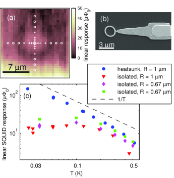
Figure 1: (color online). (a) Susceptibility scan of an isolated ring used to locate the ring and to determine the indicated measurement positions. Background measurements at positions “o” are subtracted from the data taken at positions “+” to obtain the ring response. (b) Scanning electron micrograph of a heatsunk ring. (c) Temperature dependence of the linear response of one heatsunk and three isolated rings. The data in (a) and (c) reflect the total amplitude of the linear response to a sinusoidal excitation of $\pm$45 G for (a) and the 0.67 $\mu$m rings in (c), and $\pm$35 G for the 1 $\mu$m rings.

After coarse alignment by imaging a current-carrying meander wire on the sample, accurately locating a ring is facilitated by a paramagnetic susceptibility of our metal structures that appears in scans of the linear response to an applied field [Fig. 1(a)]. To measure the complete nonlinear response, we digitized the SQUID signal at a sample rate of 333 kHz and averaged it over many sweeps of the current through the field coil, which was varied sinusoidally over the full field range at typically 111 Hz. This raw signal of a few m$\Phi_{0}$ is dominated by nonlinearities in the sensor background and a small phase shift between the fluxes applied to the two pickup loop–field coil pairs. To extract the response of a ring, we measured at the positions indicated in Fig. 1(a), and subtracted datasets taken far from the ring (o) from those near the ring (+). The total averaging time for each ring was on the order of 12 hours. The reduced coupling to the SQUID at intermediate positions was accounted for through a smaller prefactor. The symmetric measurement positions eliminate linear variations of the sensor background, which in some cases are larger and more irregular than the final signal. The reliability of the final result can be assessed by checking if its features (typically characterized by higher harmonics of the sensor response) show a spatial dependence similar to that of the ring–pickup-loop coupling. This check allowed us to identify and discard questionable datasets with very irregular features of  1 $\mu\Phi_{0}$ obtained in some sample regions.

The response of our rings is dominated by a paramagnetic linear component of up to $\approx$150 $\mu\Phi_{0}$ at a field of 45 G Bluhm et al. . Its temperature dependence is shown in Fig. 1(c). The linear response of heatsunk rings and heatsinks Bluhm et al. (not shown) varies approximately as $1/T$. Thus, it is likely due to spins. Its magnitude corresponds to a density of $4\cdot 10^{17}$ spins/m² (assuming spin 1/2). If these spins were identical to the metallic magnetic impurities that were shown to cause excess dephasing Pierre et al. (2003), one would expect a much larger spin flip dephasing rate than the upper bound obtained from our $\tau_{\phi}$ measurements.

The linear response of isolated rings varies little below $\approx$ 150 mK. This indication of a saturating electron temperature agrees with estimates of the heating effect of the  10 $\mu$A, 10 GHz Josephson current in the SQUID pickup loop aux . The different behavior of heatsunk and isolated rings shows that the linear susceptibility reflects the electron rather than phonon temperature.

We now focus on the much smaller nonlinear response, obtained after eliminating the linear response (including a component that is out-of-phase with the sinusoidal applied field) by subtracting a fitted ellipse. This linear component varied by up to a factor 2 between nominally identical rings. Fig. 2(a) shows data from fifteen isolated rings with $R$ = 0.67 $\mu$m. While these raw data are not periodic in $\Phi_{a}$, most of them can be described as the sum of a periodic component and a step-like shape near $\Phi_{a}=0$. This unexpected, poorly understood anomaly appeared in nearly all rings, and was most pronounced in heatsunk rings aux . Its frequency dependence suggests that it is due to nonequilibrium effects in the spin response, but it might mask a persistent-current-like effect aux .

Since one might expect the same spin signal from each ring, whereas persistent currents should fluctuate around a zero mean, we subtracted the average of all fifteen datasets from each individual curve. The results [Fig. 2(b)] show oscillations that can be fitted with a sine curve of the expected period for most rings. Datasets 4, 5 and 15 give better fits with a 30 % larger period, which corresponds to an effective radius close to the ring’s inner radius. This variation of the period may reflect an imperfect background elimination, but could also be a mesoscopic fluctuation of the effective ring radius. The seemingly much larger period of datasets 13 and 14 appears to be due to a different magnitude of the zero field anomaly. From the sine curve fits to 13 datasets, we obtain an estimate for $M\langle I_{h/e}^{2}\rangle^{1/2}$ of 0.11 $\mu\Phi_{0}$ if fixing the period at the value expected for the mean radius of the rings, or 0.12 $\mu\Phi_{0}$ if treating it as a free parameter. This value agrees with the theoretical value of 0.12 $\mu\Phi_{0}$ from Eq. 1 for $T$ = 150 mK, which corresponds to $\langle I_{h/e}^{2}\rangle^{1/2}=0.9$ nA for $R$ = 0.67 $\mu$m.

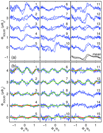
Figure 2: (color online). (a) Response of 15 nominally identical rings with $R$ = 0.67 $\mu$m after subtracting the in- and out-of-phase component of the linear response. The curve labeled “mean” is the average of datasets 1-15. (b) Results of subtracting this mean from datasets 1-15 in (a). The smooth lines are sinusoidal fits (including a linear background term) with fixed (red/dark) and fitted period (green/light). Datasets 13 and 14 were excluded from the analysis because of their stronger zero field anomaly. The rms amplitude estimated from the fixed and variable period fits corresponds to a current of 0.8 and 0.9 nA, respectively, in agreement with the expected value of $\langle I_{h/e}^{2}\rangle^{1/2}$ from Eq. 1.

We checked the reproducibility of the response over several weeks without warming up the sample for seven rings, and found good consistency in five cases. Reducing the field sweep range from 45 to 35 and 25 G or varying the frequency between 13 and 333 Hz changed the step feature, but had little effect on the oscillatory component in the difference between the responses of two rings aux .

Out of five measurements of rings with $R$ = 0.57 $\mu$m aux , four gave similar results after subtracting their mean response as the $R$ = 0.67 $\mu$m rings. The rms value of the fitted sine amplitudes was 0.06 and 0.07 $\mu\Phi_{0}$ for variable and fixed period, respectively. A fifth ring was excluded from this analysis because it had a significantly larger zero field anomaly. Data from additional three rings were rejected because of a large variation of the sensor background that was not connected with the rings.

We also measured eight isolated rings with $R$ = 1 $\mu$m, which are expected to give a smaller signal because of their smaller $E_{c}$ of 170 mK and stronger heating from the SQUID aux . Since the magnitude of the zero-field anomaly varies significantly for these rings, the mean subtraction procedure cannot fully remove it. One of these rings shows a sinusoidal signal with a period of 1 to 1.15 $\phi_{0}$ and an amplitude of up to 0.1 $\mu\Phi_{0}$, but poor reproducibility. Fitting sine curves, regardless of the absence of clear oscillations for the other seven rings, gives $M\langle I_{h/e}^{2}\rangle^{1/2}$ = 0.03 $\mu\Phi_{0}$. None of those rings show a signal at a period similar to those in Fig. 2. This dependence of the signal on the ring size supports the interpretation as persistent current, as opposed to an artifact of the spin response.

The data discussed so far was taken at base temperature. We have measured the temperature dependence of the responses of four 0.67 $\mu$m rings with large oscillatory signals of opposite sign. Taking the difference between their nonlinear responses, which eliminates any common background signal, leads to predominantly sinusoidal curves at most temperatures, as shown in Fig. 3(a). The period appears to be $T$-independent, and amplitudes from fits with a fixed period are consistent with an $e^{-k_{B}T/E_{c}}$ dependence [Fig. 3(b)] with $E_{c}/k_{B}$ = 380 mK, as obtained from the measured $D$.

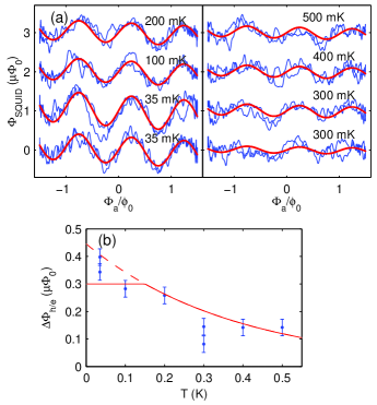
Figure 3: (color online). (a) Difference between the nonlinear responses of two rings with a large oscillatory component (curves 1 and 2 in Fig. 2) at $T$ = 0.035 K to 0.5 K. (b) Temperature dependence of the amplitude of the sinusoidal fits in panel (a). The exponential curve is a fit to $\exp(-\mathrm{min}(T,0.15K)/0.38K)$, taking the the saturation of the electron temperature into account. The error bars were obtained by analyzing the $x$ and $y$ scan across the rings [cf. Fig. 1(a)] separately and averaging the difference square of the respective results over all eight data points.

In this experiment, the $h/e$ persistent current in diffusive rings is in good agreement with theory within the temperature range covered, providing long-overdue experimental input to the questions raised by an earlier experiment Chandrasekhar et al. (1991).