One-loop QCD and electroweak corrections to $t\bar{t}Z^{0}$ production at an $e^{+}e^{-}$ linear collider

Abstract

We study the impact of the full ${\cal O}(\alpha_{s})$ QCD and ${\cal O}(\alpha_{ew})$ electroweak (EW) radiative corrections to the $e^{+}e^{-}\to t\bar{t}Z^{0}$ process in the standard model (SM), and investigate the dependence of the lowest-order(LO), one-loop QCD and EW corrected cross sections on colliding energy $\sqrt{s}$. The LO, QCD and EW corrected spectrums of the invariant mass of $t\bar{t}$-pair and the distributions of the transverse momenta of final top-quark and $Z^{0}$-boson are presented. The numerical results show that the one-loop QCD correction enhances the LO cross section, but the EW one-loop correction generally suppresses the LO cross section with our chosen parameters. In the case of $m_{H}=120~{}GeV$, the QCD relative corrections can reach $43.16\%$ when $\sqrt{s}=500~{}GeV$, while the EW relative corrections have the values of $-8.63\%$, $-4.07\%$ and $-5.42\%$, when $\sqrt{s}=500~{}GeV$, $800~{}GeV$, $1.2~{}TeV$, respectively.

PACS: 12.38.Bx, 12.15.Lk, 14.70.Hp, 14.65.Ha

I. Introduction

The standard model(SM)[1, 2] of elementary particle physics has provided a remarkably successful description of almost all available experimental data involving strong and electroweak (EW) interactions. While on the contrary, the Higgs-boson in the SM has not been discovered experimentally yet. That implies that the mechanism of the electroweak symmetry breaking (EWSB) giving masses to vector gauge bosons and fermions, remains a mystery. Moreover, the SM suffers from a few conceptional difficulties, such as hierarchy problem. This has promoted intense researches in building extension models in order to solve the hierarchy problem, and leaded to a rich phenomenology at present and future colliders.

The top-quark was discovered by the CDF and D0 collaborations at Fermilab Tevatron in 1995[3, 4]. It opens up a new research field of top physics, and confirms again the three-generation structure of the SM. But until now our knowledge about top-quark’s properties has been still limited [5]. In particular, the couplings of the top-quark to the EW gauge bosons have not yet been directly measured in high precision. Since the top-quark is the heaviest particle discovered up to now[6, 7], it indicates that among all the observed interactions of elementary particles, the top-quark mass term breaks the EW gauge symmetry maximally, and the detailed physics of the top-quark may be significantly different from the predictions provided by the SM. In other words, the top-quark probably plays a special role in EWSB. The studies of top physics could illuminate the mechanism which breaks EW symmetry. Thus we may guess the new physics connected with EWSB could be firstly found in the precision measurements involving top-quark. A possible signature for new physics could be demonstrated in the deviation of the any of the $tt\gamma$, $ttZ$ and $tbW$ couplings from the predictions of the SM. Until now there have been many works which devote to the effects of new physics on the observables related to the top-quark couplings[8, 9]. All these studies indicate that the vector and axial form factors in the couplings of top-quarks and gauge boson could receive large corrections in certain models of dynamical EW breaking[10].

As we know that it is very hard to obtain the information about the $t\bar{t}V$ $(V=Z^{0},\gamma)$ coupling from the precise measurement of the top-pair production $e^{+}e^{-}\to\gamma^{*}/Z^{*}\to t\bar{t}$ at a linear collider, because of the difficulty in distinguishing the contributions of $t\bar{t}Z^{0}$ and $t\bar{t}\gamma$ couplings. The probing of $t\bar{t}\gamma$ coupling via $\gamma\gamma\to t\bar{t}$ process was investigated in Ref.[11]. It is found that the $\gamma\gamma\to t\bar{t}$ process is sensitive to $t\bar{t}\gamma$ coupling. In references [12, 13, 14], the QCD and EW corrections to top quark pair production via fusion of both polarized and unpolarized photons in the minimal supersymmetric standard model(MSSM), are presented. The corrections are found to be sizable. At hadron colliders, a measurement of the EW neutral couplings via $q\bar{q}\to\gamma^{*}/Z^{*}\to t\bar{t}$ is hopeless due to the strong interaction process $q\bar{q}(gg)\to g^{*}\to t\bar{t}$. Instead, they can be measured in QCD $t\bar{t}Z^{0}/\gamma$ production and radiative top quark decays in $t\bar{t}$ events ($t\bar{t}\to\gamma W^{+}W^{-}b\bar{b}$). Each of the processes is sensitive to the EW couplings between top-quark and the emitted $Z^{0}$-boson(or photon)[15]. The coupling of top-quark and $Z^{0}$ gauge boson can be probed via the measurement of process $e^{+}e^{-}\to t\bar{t}Z^{0}$ at linear colliders. The process $e^{+}e^{-}\to t\bar{t}Z^{0}$ at the tree-level has been already discussed in the literature [16] by Hagiwara in the context of the SM, while CP-violating effects in $e^{+}e^{-}\to t\bar{t}Z^{0}$ process were studied in the framework of the Two Higgs Doublets Model[17] and with model independent effective Lagrangian[18]. Recently, the NLO QCD corrections to $t\bar{t}Z^{0}$ production at the LHC have been calculated in reference [19].

The International Linear Collider (ILC) is an efficient machine for precise experiments designed in $e^{+}e^{-}$ colliding energy range of $200~{}GeV<\sqrt{s}<500~{}GeV$, and it has an integrated luminosity of around $500~{}(fb)^{-1}$ in four years. It would be upgraded to $\sqrt{s}\sim 1~{}TeV$ with an integrated luminosity of $1~{}(ab)^{-1}$ in three years[20]. This machine has sufficient energy to produce top-quarks, and be ideally suited to precision studies of many top-quark properties due to the advantage of the measurement being carried out in a particularly clean environment. Thus the anomalous coupling between top-quarks and $Z^{0}$-boson can be probed by measuring precisely the $e^{+}e^{-}\to t\bar{t}Z^{0}$ process at a linear collider.

In this work we present the calculations involving the full one-loop QCD and EW corrections to the process $e^{+}e^{-}\to t\bar{t}Z^{0}$ in the SM. The paper is arranged as follows: In Section II we give the analytical calculation description of the Born cross section. The calculations of full ${\cal O}(\alpha_{s})$ QCD and ${\cal O}(\alpha_{ew})$ electroweak radiative corrections to $t\bar{t}Z^{0}$ production at an $e^{+}e^{-}$ linear collider are provided in Section III and IV, respectively. In Section V we present some numerical results and discussions, and finally a short summary is given.

II. LO calculation for $e^{+}e^{-}\to t\bar{t}Z^{0}$ process

We use the ’t Hooft-Feynman gauge in the leading-order calculation, except when we verify the gauge invariance. The contribution to the cross section of process $e^{+}e^{-}\to t\bar{t}Z^{0}$ in the SM at the lowest order is of the order ${\cal O}(\alpha_{ew}^{3})$ with pure electroweak interactions. There are totally nine tree-level Feynman diagrams, which are drawn in Fig.1. The Feynman diagrams in Fig.1 topologically can be divided into s-channel(Fig.1(1)-(5)) and t(u)-channel(Fig.1(6)-(9)) diagrams.

Figure 1: The lowest order diagrams for the $e^{+}e^{-}\to t\bar{t}Z^{0}$ process in the SM.

We define the notations for the process $e^{+}e^{-}\to t\bar{t}Z^{0}$ as

$$e^{+}(p_{1})+e^{-}(p_{2})\to t(k_{1})+\bar{t}(k_{2})+Z^{0}(k_{3}),$$ (2.1)

where the four-momenta of incoming positron and electron are represented as $p_{1}$ and $p_{2}$, respectively, and the four-momenta of outgoing top-quark, anti-top-quark and $Z^{0}$-boson are denoted as $k_{1}$, $k_{2}$ and $k_{3}$ correspondingly. All these momenta obey the on-shell equations $p_{1}^{2}=p_{2}^{2}=m_{e}^{2}$, $k_{1}^{2}=k_{2}^{2}=m_{t}^{2}$ and $k_{3}^{2}=m_{Z}^{2}$.

The amplitudes of the corresponding tree-level Feynman diagrams for the process $e^{+}e^{-}\to t\bar{t}Z^{0}$ shown in Fig.1, are respectively expressed as

$${\cal M}^{(1)} = \frac{ie^{3}m_{t}}{8s_{W}^{3}c_{W}^{3}}\times\frac{1}{\left(s-m_{Z}^{2}\right)\left[(k_{1}+k_{2})^{2}-m_{H}^{2}\right]}\bar{u}(k_{1})v(k_{2})\bar{v}(p_{1})\gamma_{\mu}\left(1-4s_{W}^{2}-\gamma_{5}\right)~{}~{}~{}~{}$$ (2.2)

$$\times u(p_{2})\epsilon^{\mu}(k_{3}),$$

$${\cal M}^{(2)} = \frac{-ie^{3}}{6s_{W}c_{W}}\times\frac{1}{s\left[(k_{1}+k_{3})^{2}-m_{t}^{2}\right]}\bar{u}(k_{1})\gamma_{\mu}\left(1-\frac{8}{3}s_{W}^{2}-\gamma_{5}\right)(\hbox to0.0pt{/\hss}k_{1}+\hbox to0.0pt{/\hss}k_{3}+m_{t})~{}~{}~{}~{}$$ (2.3)

$$\times \gamma_{\nu}v(k_{2})\bar{v}(p_{1})\gamma^{\nu}u(p_{2})\epsilon^{\mu}(k_{3}),$$

$${\cal M}^{(3)} = \frac{-ie^{3}}{64s_{W}^{3}c_{W}^{3}}\times\frac{1}{\left(s-m_{Z}^{2}\right)\left[(k_{1}+k_{3})^{2}-m_{t}^{2}\right]}\bar{u}(k_{1})\gamma_{\mu}\left(1-\frac{8}{3}s_{W}^{2}-\gamma_{5}\right)(\hbox to0.0pt{/\hss}k_{1}+\hbox to0.0pt{/\hss}k_{3}+m_{t})~{}~{}~{}~{}$$ (2.4)

$$\times \gamma^{\nu}\left(1-\frac{8}{3}s_{W}^{2}-\gamma_{5}\right)v(k_{2})\bar{v}(p_{1})\gamma_{\nu}\left(1-4s_{W}^{2}-\gamma_{5}\right)u(p_{2})\epsilon^{\mu}(k_{3}),$$

$${\cal M}^{(4)} = \frac{-ie^{3}}{6s_{W}c_{W}}\times\frac{1}{s\left[(k_{2}+k_{3})^{2}-m_{t}^{2}\right]}\bar{u}(k_{1})\gamma^{\nu}(-\hbox to0.0pt{/\hss}k_{2}-\hbox to0.0pt{/\hss}k_{3}+m_{t})\gamma_{\mu}\left(1-\frac{8}{3}s_{W}^{2}-\gamma_{5}\right)~{}~{}~{}~{}$$ (2.5)

$$\times v(k_{2})\bar{v}(p_{1})\gamma_{\nu}u(p_{2})\epsilon^{\mu}(k_{3}),$$

$${\cal M}^{(5)} = \frac{-ie^{3}}{64s_{W}^{3}c_{W}^{3}}\times\frac{1}{\left(s-m_{Z}^{2}\right)\left[(k_{2}+k_{3})^{2}-m_{t}^{2}\right]}\bar{u}(k_{1})\gamma^{\nu}\left(1-\frac{8}{3}s_{W}^{2}-\gamma_{5}\right)(-\hbox to0.0pt{/\hss}k_{2}-\hbox to0.0pt{/\hss}k_{3}+m_{t})\gamma_{\mu}~{}~{}~{}~{}$$ (2.6)

$$\times \left(1-\frac{8}{3}s_{W}^{2}-\gamma_{5}\right)v(k_{2})\bar{v}(p_{1})\gamma_{\nu}\left(1-4s_{W}^{2}-\gamma_{5}\right)u(p_{2})\epsilon^{\mu}(k_{3}),$$

$${\cal M}^{(6)} = \frac{ie^{3}}{6s_{W}c_{W}}\times\frac{1}{(k_{1}+k_{2})^{2}\left[(p_{2}-k_{3})^{2}-m_{e}^{2}\right]}\bar{u}(k_{1})\gamma^{\nu}v(k_{2})\bar{v}(p_{1})\gamma_{\nu}(\hbox to0.0pt{/\hss}p_{2}-\hbox to0.0pt{/\hss}k_{3}+m_{e})~{}~{}~{}~{}$$ (2.7)

$$\times \gamma_{\mu}\left(1-4s_{W}^{2}-\gamma_{5}\right)u(p_{2})\epsilon^{\mu}(k_{3}),$$

$${\cal M}^{(7)} = \frac{ie^{3}}{64s_{W}^{3}c_{W}^{3}}\times\frac{1}{\left[(k_{1}+k_{2})^{2}-m_{Z}^{2}\right]\left[(p_{2}-k_{3})^{2}-m_{e}^{2}\right]}\bar{u}(k_{1})\gamma^{\nu}\left(1-\frac{8}{3}s_{W}^{2}-\gamma_{5}\right)v(k_{2})\bar{v}(p_{1})\gamma_{\nu}~{}~{}~{}~{}$$ (2.8)

$$\times \left(1-4s_{W}^{2}-\gamma_{5}\right)(\hbox to0.0pt{/\hss}p_{2}-\hbox to0.0pt{/\hss}k_{3}+m_{e})\gamma_{\mu}\left(1-4s_{W}^{2}-\gamma_{5}\right)u(p_{2})\epsilon^{\mu}(k_{3}),$$

$${\cal M}^{(8)} = \frac{ie^{3}}{6s_{W}c_{W}}\times\frac{1}{(k_{1}+k_{2})^{2}\left[(p_{1}-k_{3})^{2}-m_{e}^{2}\right]}\bar{u}(k_{1})\gamma^{\nu}v(k_{2})\bar{v}(p_{1})\gamma_{\mu}(-\hbox to0.0pt{/\hss}p_{1}+\hbox to0.0pt{/\hss}k_{3}+m_{e})~{}~{}~{}~{}$$ (2.9)

$$\times \gamma_{\nu}\left(1-4s_{W}^{2}-\gamma_{5}\right)u(p_{2})\epsilon^{\mu}(k_{3}),$$

$${\cal M}^{(9)} = \frac{ie^{3}}{64s_{W}^{3}c_{W}^{3}}\times\frac{1}{\left[(k_{1}+k_{2})^{2}-m_{Z}^{2}\right]\left[(p_{1}-k_{3})^{2}-m_{e}^{2}\right]}\bar{u}(k_{1})\gamma^{\nu}\left(1-\frac{8}{3}s_{W}^{2}-\gamma_{5}\right)v(k_{2})\bar{v}(p_{1})~{}~{}~{}~{}$$ (2.10)

$$\times \gamma_{\mu}\left(1-4s_{W}^{2}-\gamma_{5}\right)(-\hbox to0.0pt{/\hss}p_{1}+\hbox to0.0pt{/\hss}k_{3}+m_{e})\gamma_{\nu}\left(1-4s_{W}^{2}-\gamma_{5}\right)u(p_{2})\epsilon^{\mu}(k_{3}).$$

Then the total amplitude at the lowest order can be obtained by summing up all the above amplitudes given in Eqs.(2.2)-(2.10).

$${\cal M}_{0}=\sum_{i=1}^{9}{\cal M}^{(i)}.$$ (2.11)

The differential cross section for the process $e^{+}e^{-}\to t\bar{t}Z^{0}$ at the tree-level with unpolarized incoming particles is then obtained as

$$d\sigma_{0}=\frac{N_{c}}{4}\sum_{spins}|{\cal M}_{0}|^{2}d\Phi_{3},$$ (2.12)

where the color number $N_{c}=3$, the summation is taken over the spins of initial and final particles. The factor $\frac{1}{4}$ is due to taking average over the polarization states of the electron and positron. $d\Phi_{3}$ is the three-particle phase space element defined as

$$d\Phi_{3}=\delta^{(4)}\left(p_{1}+p_{2}-\sum_{i=1}^{3}k_{i}\right)\prod_{j=1}^{3}\frac{d^{3}\textbf{{k}}_{j}}{(2\pi)^{3}2E_{j}}.$$ (2.13)

III. One-loop QCD corrections to the $e^{+}e^{-}\to t\bar{t}Z^{0}$ process

Figure 2: The box and triangle diagrams of one-loop QCD corrections to the $e^{+}e^{-}\to t\bar{t}Z^{0}$ process.

The QCD one-loop Feynman diagrams and corresponding amplitudes of the process $e^{+}e^{-}\to t\bar{t}Z^{0}$ are generated by using FeynArts3.2 [21]. We present the box and triangle diagrams of one-loop QCD corrections to the $e^{+}e^{-}\to t\bar{t}Z^{0}$ process in Fig.2. We take the definitions of one-loop integral functions in Ref.[22], and use mainly the FormCalc4.1 package[23] to calculate the amplitudes of one-loop Feynman diagrams and get the results in a way well suited for further numerical or analytical evaluation. The calculation of the amplitude for one-loop diagram has been performed in the conventional ’t Hooft–Feynman gauge by adopting dimension regularization scheme in which the dimensions of spinor and space-time manifolds are extended to $D=4-2\epsilon$. The numerical calculations of the integral functions are implemented by using our in-house programs developed from the FF package[24]. In these programs, the numerical evaluations of one-point, two-point, three-point and four-point integrals are evaluated by using the expressions from Ref.[25], and the scalar and tensor 5-point integrals are calculated exactly by using the approach presented in Ref.[26]. The phase space integration for the process $e^{+}e^{-}\to t\bar{t}Z^{0}$ is implemented by adopting 2to3.F subroutine in FormCalc4.1 package. In the calculation of the correction from the hard gluon emission process $e^{+}e^{-}\to t\bar{t}Z^{0}g$ , we use CompHEP-4.4p3 program[27] to generate all the tree-level diagrams and their corresponding amplitudes automatically, and accomplish the four-body phase-space integration. In CompHEP-4.4p3 and 2to3.F programs the well-known adaptive Monte Carlo method (the VEGAS algorithm) is adopted for multi-particle phase space integration[28]. Then we can obtain the NLO QCD corrected total and differential cross sections. The amplitude of the process $e^{+}e^{-}\to t\bar{t}Z^{0}$ including virtual QCD corrections at ${\cal O}(\alpha_{s})$ order can be expressed as

$${\cal M}_{QCD}={\cal M}_{0}+{\cal M}_{QCD}^{vir},$$ (3.1)

where ${\cal M}_{QCD}^{vir}$ is the renormalized amplitude contributed by the QCD one-loop Feynman diagrams and their corresponding counterterms. The relevant renormalization constants for top field are defined as

$$t_{0}^{L}=(1+\frac{1}{2}\delta Z_{t,{QCD}}^{L})t^{L},~{}~{}t_{0}^{R}=(1+\frac{1}{2}\delta Z_{t,{QCD}}^{R})t^{R}.$$ (3.2)

Taking the on-mass-shell renormalized condition we get the ${\cal O}(\alpha_{s})$ QCD contributed parts of the renormalization constants as

$$\delta Z_{t,{QCD}}^{L}=-\tilde{Re}\Sigma_{t,{QCD}}^{L}(m_{t}^{2})-m_{t}^{2}\frac{\partial}{\partial p^{2}}\tilde{Re}\left[\Sigma_{t,{QCD}}^{L}(p^{2})+\Sigma_{t,{QCD}}^{R}(p^{2})+2\Sigma_{t,{QCD}}^{S}(p^{2})\right]|_{p^{2}=m_{t}^{2}},$$ (3.3)

$$\delta Z_{t,{QCD}}^{R}=-\tilde{Re}\Sigma_{t,{QCD}}^{R}(m_{t}^{2})-m_{t}^{2}\frac{\partial}{\partial p^{2}}\tilde{Re}\left[\Sigma_{t,{QCD}}^{L}(p^{2})+\Sigma_{t,{QCD}}^{R}(p^{2})+2\Sigma_{t,{QCD}}^{S}(p^{2})\right]|_{p^{2}=m_{t}^{2}},$$ (3.4)

where $\tilde{Re}$ represents taking the real part of the loop integrals appearing in the self-energies only, and the renormalized top-quark irreducible QCD two-point function is defined as

$$\hat{\Gamma}_{t,{QCD}}(p^{2})=i\left[\hbox to0.0pt{/\hss}pP_{L}\hat{\Sigma}_{t,{QCD}}^{L}(p^{2})+\hbox to0.0pt{/\hss}pP_{R}\hat{\Sigma}_{t,{QCD}}^{R}(p^{2})+m_{t}\hat{\Sigma}_{t,{QCD}}^{S}(p^{2})\right]\delta_{\alpha\beta}$$ (3.5)

where $\alpha$ and $\beta$ are the color indices of the top-quarks on the two sides of the self-energy diagram, and $P_{L,R}=(1\mp\gamma_{5})/2$. The unrenormalized top-quark QCD self-energy parts at QCD one-loop order read

$$\Sigma_{t,{QCD}}^{L}(p^{2})=\Sigma_{t,{QCD}}^{R}(p^{2})=\frac{g_{s}^{2}C_{F}}{16\pi^{2}}\left(-1+2B_{0}[p,0,m_{t}]+2B_{1}[p,0,m_{t}]\right),$$ (3.6)

and

$$\Sigma_{t,{QCD}}^{S}(p^{2})=\frac{g_{s}^{2}C_{F}}{8\pi^{2}}\left(1-2B_{0}[p,0,m_{t}]\right).$$ (3.7)

The corresponding contribution part to the cross section at ${\cal O}(\alpha_{s})$ order can be written as

$$\Delta\sigma^{QCD}_{vir}=\sigma_{0}\delta^{QCD}_{vir}=\frac{(2\pi)^{4}N_{c}}{2|\vec{p}_{1}|\sqrt{s}}\int{\rm d}\Phi_{3}\overline{\sum_{spins}}{\rm Re}\left({\cal M}_{0}^{{\dagger}}{\cal M}_{QCD}^{vir}\right),$$ (3.8)

where $N_{c}=3$, $C_{F}=4/3$, and the bar over summation recalls averaging over the spins of incoming particles.

The virtual QCD correction contains ultraviolet (UV) and infrared (IR) divergences. The UV divergences from one-loop diagrams can be cancelled after the renormalization by adopting the dimensional regularization. We have verified the UV finiteness for the renormalized amplitude analytically and numerically.

The IR divergences in the ${\cal M}_{QCD}^{vir}$ are originated from the contributions of virtual gluon exchange in loops. These IR divergencies can be cancelled by the real gluon bremsstrahlung corrections in the soft gluon limit, due to the Kinoshita-Lee-Nauenberg (KLN) theorem[29]. In our calculation these IR divergencies are regulated by a small gluon mass. The real gluon emission process is denoted as

$$e^{+}(p_{1})+e^{-}(p_{2})\to t(k_{1})+\bar{t}(k_{2})+Z^{0}(k_{3})+g(k),$$ (3.9)

where the real gluon radiates from top(anti-top) quark line. We adopt the phase-space-slicing method [31] to isolate the IR soft singularity. The cross section of the real gluon emission process (3.9) is decomposed into soft and hard terms

$$\Delta\sigma_{real}^{QCD}=\Delta\sigma_{soft}^{QCD}+\Delta\sigma_{hard}^{QCD}.$$ (3.10)

In practice, we take a very small value for the cutoff $\Delta E_{g}/E_{b}$ in the numerical calculations, and neglect the terms of order $\Delta E_{g}/E_{b}$ in evaluating the following integration for soft contribution[22, 25, 32],

$${d}\Delta\sigma_{soft}^{QCD}=-d\sigma_{{0}}\frac{\alpha_{s}C_{F}}{2\pi^{2}}\int_{E_{g}\leq\Delta E_{g}}\frac{d^{3}k}{2E_{g}}\left(\frac{k_{1}}{k_{1}\cdot k}-\frac{k_{2}}{k_{2}\cdot k}\right)^{2},$$ (3.11)

where $E_{g}\leq\Delta E_{g}\ll\sqrt{s}$, $\Delta E_{g}$ is the energy cutoff of the soft gluon, and the gluon energy can be obtained by $E_{g}=\sqrt{|\vec{k}|^{2}+m_{g}^{2}}$.

The cancelation of the IR divergencies in the virtual contribution part and the soft gluon bremsstrahlung correction, can be verified during our calculation. Thus we get an IR finite cross section which is independent of the infinitesimal fictitious gluon mass $m_{g}$. The hard gluon emission cross section $\Delta\sigma^{QCD}_{hard}$ is calculated numerically by using Monte Carlo program in CompHEP-4.4p3 package.

The UV and IR finite total cross section of the process $e^{+}e^{-}\to t\bar{t}Z^{0}$ including the ${\cal O}(\alpha_{s})$ QCD contributions reads

$$\sigma^{QCD}=\sigma_{0}+\Delta\sigma^{QCD}=\sigma_{0}+\Delta\sigma_{vir}^{QCD}+\Delta\sigma_{soft}^{QCD}+\Delta\sigma_{hard}^{QCD}=\sigma_{0}(1+\delta^{QCD}),$$ (3.12)

where $\Delta\sigma^{QCD}$ and $\delta^{QCD}$ are the QCD cross section correction and QCD relative correction at the order of ${\cal O}(\alpha_{s})$, respectively.

IV. One-loop EW corrections to the $e^{+}e^{-}\to t\bar{t}Z^{0}$ process

In this section, we present the calculation of the ${\cal O}(\alpha_{ew})$ order EW corrections to the process $e^{+}e^{-}\to t\bar{t}Z^{0}$ . We use again the package FeynArts3.2 to generate the one-loop EW Feynman diagrams and the relevant amplitudes of the process $e^{+}e^{-}\to t\bar{t}Z^{0}$ . The one-loop EW Feynman diagrams can be classified into self-energy, triangle, box, pentagon and counterterm diagrams. Some pentagon diagrams are depicted in Fig.3 as a representative selection. In our EW correction calculation we adopt the t’Hooft-Feynman gauge and the same definitions of one-loop integral functions as in Ref.[22]. We take the dimensional regularization scheme to regularize the UV divergences in loop integrals, and assume that the CKM matrix is identity matrix and use the on-mass-shell(OMS) renormalization scheme [22]. The relevant field and mass renormalization constants are defined as

$$e_{0}=(1+\delta Z_{e})e,~{}~{}~{}m_{f,0}=m_{f}+\delta m_{f},~{}~{}~{}m_{W(Z),0}^{2}=m_{W(Z)}^{2}+\delta m_{W(Z)}^{2},~{}~{}~{}H_{0}=(1+\frac{1}{2}\delta Z_{H})H,~{}~{}~{}$$

$$A_{0}=\frac{1}{2}\delta Z_{AZ}Z+(1+\frac{1}{2}\delta Z_{AA})A,~{}~{}~{}Z_{0}=(1+\frac{1}{2}\delta Z_{ZZ})Z+\frac{1}{2}\delta Z_{ZA}A,~{}~{}~{}~{}~{}~{}~{}~{}~{}~{}~{}~{}$$

$$f_{0}^{L}=(1+\frac{1}{2}\delta Z_{f}^{L})f^{L},~{}~{}~{}~{}f_{0}^{R}=(1+\frac{1}{2}\delta Z_{f}^{R})f^{R}.~{}~{}~{}~{}~{}~{}~{}~{}~{}~{}~{}~{}~{}~{}~{}$$ (4.1)

With the on-mass-shell conditions, we can obtain the related renormalized constants expressed as

$$\delta m_{f}=\frac{m_{f}}{2}\tilde{Re}\left[\Sigma_{f}^{L}(m_{f}^{2})+\Sigma_{f}^{R}(m_{f}^{2})+2\Sigma_{f}^{S}(m_{f}^{2})\right],~{}~{}~{}~{}~{}~{}~{}~{}~{}$$

$$\delta m_{W}^{2}=\tilde{Re}\Sigma_{T}^{W}(m_{W}^{2}),~{}~{}~{}\delta m_{Z}^{2}=Re\Sigma_{T}^{ZZ}(m_{Z}^{2}),~{}~{}~{}\delta Z_{H}=-Re\frac{\partial\Sigma^{H}(k^{2})}{\partial k^{2}}|_{k^{2}=m_{H}^{2}},~{}~{}~{}$$

$$\delta Z_{AA}=-\frac{\partial\Sigma_{T}^{AA}(p^{2})}{\partial p^{2}}|_{p^{2}=0},~{}~{}~{}\delta Z_{ZZ}=-Re\frac{\partial\Sigma_{T}^{ZZ}(p^{2})}{\partial p^{2}}|_{p^{2}=m_{Z}^{2}},~{}~{}~{}$$

$$\delta Z_{ZA}=2\frac{\Sigma_{T}^{ZA}(0)}{m_{Z}^{2}},~{}~{}~{}\delta Z_{AZ}=-2Re\frac{\Sigma_{T}^{AZ}(m_{Z}^{2})}{m_{Z}^{2}}.$$ (4.2)

The charge renormalization constant and the counterterm of the parameter $s_{W}$ can be obtained by using following equations[22]:

$$\delta Z_{e}=-\frac{1}{2}\delta Z_{AA}-\frac{s_{W}}{c_{W}}\frac{1}{2}\delta Z_{ZA},~{}~{}~{}\frac{\delta s_{W}}{s_{W}}=-\frac{1}{2}\frac{c_{W}^{2}}{s_{W}^{2}}\tilde{Re}\left(\frac{\Sigma_{T}^{W}(m_{W}^{2})}{m_{W}^{2}}-\frac{\Sigma_{T}^{ZZ}(m_{Z}^{2})}{m_{Z}^{2}}\right).$$ (4.3)

We use Eqs.(3.3)-(3.4) to calculate the renormalization constants of the fermion wave functions, but the top-quark QCD self-energies in these equations($\Sigma_{t,{QCD}}^{L}$, $\Sigma_{t,{QCD}}^{R}$ and $\Sigma_{t,{QCD}}^{S}$) are replaced by the corresponding fermion EW self-energies($\Sigma_{f,EW}^{L}$, $\Sigma_{f,EW}^{R}$ and $\Sigma_{f,EW}^{S}$), respectively. And the explicit expressions of the relevant EW self-energies in the SM can be found in the Appendix B of Ref.[22]. The UV divergence appearing from the one-loop diagrams should be cancelled by the contributions of the counterterm diagrams. In our calculations, it was verified both analytically and numerically that the total cross sections including ${\cal O}(\alpha_{ew})$ one-loop radiative corrections and the corresponding counterterm contributions, are UV finite. Then the one-loop level virtual EW corrections to the cross section can be expressed as

$$\Delta\sigma^{EW}_{{\rm vir}}=\sigma_{0}\delta^{EW}_{vir}=\frac{(2\pi)^{4}N_{c}}{2|\vec{p}_{1}|\sqrt{s}}\int{\rm d}\Phi_{3}\overline{\sum_{spins}}{\rm Re}\left({\cal M}^{{\dagger}}_{0}{\cal M}^{EW}_{{\rm vir}}\right),$$ (4.4)

where $\vec{p}_{1}$ is the c.m.s. three-momentum of the incoming positron, ${\rm d}\Phi_{3}$ is the three-body phase space element, and the bar over summation denotes averaging over initial spins. ${\cal M}^{EW}_{{\rm vir}}$ is the renormalized total amplitude of all the one-loop EW level Feynman diagrams, including self-energy, vertex, box, pentagon and counterterm diagrams.

Figure 3: Some representative pentagon one-loop EW diagrams for the $e^{+}e^{-}\to t\bar{t}Z^{0}$ process.

Analogous to the calculation of the QCD correction as described in above section, we generate the EW one-loop Feynman diagrams and calculate their amplitudes for $e^{+}e^{-}\to t\bar{t}Z^{0}$ process by using FeynArts3.2 and FormCalc4.1 packages. The numerical calculations of integral functions are performed by adopting our in-house library. The phase space of process $e^{+}e^{-}\to t\bar{t}Z^{0}$ is integrated by using 2to3.F subroutine. In calculating the correction from hard photon emission process $e^{+}e^{-}\to t\bar{t}Z^{0}\gamma$ , the CompHEP-4.4p3 program is used to generate the tree-level diagrams and amplitudes, and carry out the integration in four-body phase-space. During the calculation of the EW corrections to the process $e^{+}e^{-}\to t\bar{t}Z^{0}$ , the IR divergence originating from virtual photon correction should be canceled by the real photon bremsstrahlung correction in the soft photon limit. We use also the phase-space-slicing method and divide the cross section of the real photon emission process, denoted as $e^{+}(p_{1})e^{-}(p_{2})\to t(k_{1})\bar{t}(k_{2})Z^{0}(k_{3})\gamma(k)$, into soft and hard parts.

$$\Delta\sigma_{{\rm real}}^{EW}=\Delta\sigma_{soft}^{EW}+\Delta\sigma_{hard}^{EW}=\sigma_{0}(\delta^{EW}_{soft}+\delta^{EW}_{hard}).$$ (4.5)

By using the soft photon($E_{\gamma}<\Delta E_{\gamma}$) approximation, we get the contribution of the soft photon emission process expressed as

$${\rm d}\Delta\sigma^{EW}_{soft}=-{\rm d}\sigma_{0}\frac{\alpha_{ew}}{2\pi^{2}}\int_{E_{\gamma}\leq\Delta E_{\gamma}}\frac{{\rm d}^{3}k}{2E_{\gamma}}\left[\frac{Q_{t}k_{1}}{k_{1}\cdot k}-\frac{Q_{t}k_{2}}{k_{2}\cdot k}-\frac{p_{1}}{p_{1}\cdot k}+\frac{p_{2}}{p_{2}\cdot k}\right]^{2},$$ (4.6)

in which $\Delta E_{\gamma}$ is the energy cutoff of the soft photon and $E_{\gamma}\leq\Delta E_{\gamma}\ll\sqrt{s}$, $Q_{t}=2/3$ is the electric charge of top quark, $E_{\gamma}=\sqrt{|\vec{k}|^{2}+m_{\gamma}^{2}}$ is the photon energy. Therefore, after integrating approximately over the soft photon phase space, we can obtain the analytical result of the soft photon emission corrections to $e^{+}e^{-}\to t\bar{t}Z^{0}$ . The cancellation of IR divergencies is verified and the results shows that the cross section for $e^{+}e^{-}\to t\bar{t}Z^{0}g$ is independent on the infinitesimal photon mass $m_{\gamma}$ in our calculation.

For the convenience in analyzing the origins of the EW radiation corrections, we split the full one-loop EW level correction into the QED correction part ($\Delta\sigma^{E}$) and the pure weak correction part ($\Delta\sigma^{W}$). The QED correction part involves the contributions from the one-loop diagrams with virtual photon exchange in loop, the real photon emission process $e^{+}e^{-}\to t\bar{t}Z^{0}\gamma$ , and the pure photonic contribution of the renormalization constants of the related fermions. The rest of the total EW corrections remains with the weak correction part. Then we can express the full one-loop EW corrected total cross section as

$$\Delta\sigma^{EW}=\Delta\sigma^{E}+\Delta\sigma^{W}.$$ (4.7)

V. Numerical Results and Discussion

In the following numerical calculation, we have used the 3-loop evolution of strong coupling constant $\alpha_{s}(\mu^{2})$ in the $\overline{MS}$ scheme with parameters $\Lambda_{QCD}^{n_{f}=5}=203.73~{}MeV$, yielding $\alpha_{s}^{\overline{MS}}(m_{Z}^{2})=0.1176$. We take the relevant parameters as[6, 7] : $\alpha_{{\rm ew}}(0)^{-1}=137.036$, $m_{e}=0.519991~{}MeV$, $m_{\mu}=105.6583692~{}MeV$, $m_{\tau}=1.77699~{}GeV$, $m_{W}=80.403~{}GeV$, $m_{Z}=91.1876~{}GeV$, $m_{t}=172.5~{}GeV$, $m_{s}=150~{}GeV$, $m_{c}=1.2~{}GeV$, $m_{b}=4.7~{}GeV$, $m_{u}=m_{d}=66~{}MeV$, $\sin^{2}\theta_{W}=1-m_{W}^{2}/m_{Z}^{2}=0.222549$, and $\mu=m_{t}+\frac{1}{2}m_{Z}$. There the light quark masses ($m_{u}$ and $m_{d}$) have the effective values which can reproduce the hadron contribution to the shift in the fine structure constant $\alpha_{ew}(m_{Z}^{2})$[33]. With above parameter choice we get $\alpha_{s}(\mu^{2}=(m_{t}+\frac{1}{2}m_{Z})^{2})=0.1040$. Since LEP II and the electroweak precision measurements have provided that the SM Higgs-boson exists in the mass range of $114.4~{}GeV<m_{H}\lesssim 182~{}GeV$[34, 35], we include the relevant Higgs contributions with $m_{H}=120~{}GeV$ as a representation.

During our calculation of one-loop corrections, we have to fix the values of the fictitious masses of photon and gluon(as IR regulators $m_{\gamma}$ and $m_{g}$), and soft cutoff $\delta_{s}=\Delta E_{g(\gamma)}/E_{b}$ except the input parameters mentioned above. In fact, the physical total cross section should be independent of these regulators and soft cutoff. We have verified the invariance of the cross section contributions at QCD and EW one-loop order, $\Delta\sigma^{QCD,EW}_{tot}=\Delta\sigma_{real}^{QCD,EW}+\Delta\sigma_{vir}^{QCD,EW}$, within the calculation errors when the fictitious photon and gluon masses, $m_{\gamma}$ and $m_{g}$, vary from $10^{-10}~{}GeV$ to $10^{-1}~{}GeV$ in conditions of $\delta_{s}=2\times 10^{-3}$, $m_{H}=120~{}GeV$ and $\sqrt{s}=500~{}GeV$. The relation between the ${\cal O}(\alpha_{s})$ QCD (${\cal O}(\alpha_{ew})$ EW) correction and soft cutoff $\delta_{s}$ demonstrates in Figs.4(a-b) (Figs.5(a-b)), assuming $m_{g}=10^{-3}~{}GeV$ ($m_{\gamma}=10^{-3}~{}GeV$), $m_{H}=120~{}GeV$ and $\sqrt{s}=500~{}GeV$. We can see in Fig.4(a) and Fig.5(a) that the curves for $\Delta\sigma^{QCD,EW}_{soft}+\Delta\sigma^{QCD,EW}_{vir}$ and $\Delta\sigma^{QCD,EW}_{hard}$ are strongly related to the soft cutoff $\delta_{s}$, but both the total QCD and EW one-loop radiative corrections, $\Delta\sigma^{QCD,EW}(\equiv\Delta\sigma^{QCD,EW}_{vir}+\Delta\sigma^{QCD,EW}_{soft}+\Delta\sigma^{QCD,EW}_{hard})$, are independent of the cutoff $\delta_{s}$ within the range of calculation errors as we expected. In Fig.4(b) and Fig.5(b), we make the curves for $\Delta\sigma^{QCD}$ and $\Delta\sigma^{EW}$ greater in size and mark them with the calculation errors, respectively. In the further calculation, we fix the soft cutoff, fictitious photon and gluon masses as $\delta_{s}=2\times 10^{-3}$, $m_{\gamma}=10^{-1}~{}GeV$ and $m_{g}=10^{-2}~{}GeV$.

Figure 4: (a) The ${\cal O}(\alpha_{s})$ QCD corrections to the cross section for $e^{+}e^{-}\to t\bar{t}Z^{0}$ as the functions of the soft cutoff $\delta_{s}\equiv\Delta E_{g}/E_{b}$ in conditions of $m_{g}=10^{-3}~{}GeV$, $m_{H}=120~{}GeV$ and $\sqrt{s}=500~{}GeV$. (b) The amplified curve marked with the calculation errors for $\Delta\sigma^{QCD}$ of Fig.4(a) versus $\delta_{s}$.

Figure 5: (a) The ${\cal O}(\alpha_{ew})$ EW corrections to the cross section for $e^{+}e^{-}\to t\bar{t}Z^{0}$ as the functions of the soft cutoff $\delta_{s}\equiv\Delta E_{\gamma}/E_{b}$ in conditions of $m_{\gamma}=10^{-3}~{}GeV$, $m_{H}=120~{}GeV$ and $\sqrt{s}=500~{}GeV$. (b) The amplified curve marked with the calculation errors for $\Delta\sigma^{EW}$ of Fig.5(a) versus $\delta_{s}$.

In order to verify the reliability of our calculations for the tree-level cross section of process $e^{+}e^{-}\to t\bar{t}Z^{0}$ , the QCD correction from hard gluon emission process $e^{+}e^{-}\to t\bar{t}Z^{0}g$ and the EW correction from hard photon emission process $e^{+}e^{-}\to t\bar{t}Z^{0}\gamma$ , we evaluated their numerical results by adopting different gauges and software tools. In Table 1, we list these numerical results by taking $m_{H}=120~{}GeV$ and $\sqrt{s}=500~{}GeV$, and using CompHEP-4.4p3 program[27] (in both Feynman and unitary gauges), FeynArts3.2/FormCalc4.1 [21, 23](in Feynman gauge, and the phase space integrations are implemented by using 2to3.F subroutine for $e^{+}e^{-}\to t\bar{t}Z^{0}$ process and in-house $2\to 4$ phase space integration program for $e^{+}e^{-}\to t\bar{t}Z^{0}g$ and $e^{+}e^{-}\to t\bar{t}Z^{0}\gamma$ processes.) and Grace2.2.1[36] package(in Feynman gauge), separately. We can see the results are in mutual agreement within the phase space integration errors. We have calculated also the tree-level cross section for the $e^{+}e^{-}\to t\bar{t}Z^{0}$ process by taking the same input parameters as in Ref.[16], and got coincident numerical results.

	CompHEP	CompHEP	FeynArts	Grace
	Feynman Gauge	Unitary Gauge	Feynman Gauge	Feynman Gauge
$\sigma_{0}$ (fb)	1.0649(1)	1.0648(1)	1.0648(2)	1.0647(2)
$\Delta\sigma_{hard}^{QCD}$ (fb)	$7.028(2)\times 10^{-2}$	$7.028(2)\times 10^{-2}$	$7.028(2)\times 10^{-2}$	$7.028(2)\times 10^{-2}$
$\Delta\sigma_{hard}^{EW}$ (fb)	$0.4631(2)$	$0.4632(2)$	$0.4631(2)$	$0.4632(2)$

Table 1: The comparison of the results for the tree-level cross section for the process $e^{+}e^{-}\to t\bar{t}Z^{0}$ ($\sigma_{0}$) and the corrections from hard gluon/photon emission processes $e^{+}e^{-}\to t\bar{t}Z^{0}g$ ($\Delta\sigma_{hard}^{QCD}$) and $e^{+}e^{-}\to t\bar{t}Z^{0}\gamma$ ($\Delta\sigma_{hard}^{EW}$), in conditions of $m_{H}=120~{}GeV$, $\sqrt{s}=500~{}GeV$ and $\delta_{s}=2\times 10^{-3}$. The numerical results are obtained by using CompHEP-4.4p3(in both Feynman and unitary gauges), FeynArts3.2/FormCalc4.1(in Feynman gauge, the phase space integrations are implemented by using 2to3.F subroutine for $e^{+}e^{-}\to t\bar{t}Z^{0}$ process and in-house $2\to 4$ phase space integration program for $e^{+}e^{-}\to t\bar{t}Z^{0}g$ and $e^{+}e^{-}\to t\bar{t}Z^{0}\gamma$ processes) and Grace2.2.1(in Feynman gauge) packages, separately.

For the check of the calculations for one-loop diagrams, we used the LoopTools2.2 library and our in-house program(Both are in two combination cases respectively) to calculate the one-loop QCD and EW corrections to the process $e^{+}e^{-}\to t\bar{t}Z^{0}$ ($\Delta\sigma^{QCD,EW}_{soft}+\Delta\sigma^{QCD,EW}_{vir}$) numerically, in conditions of $m_{H}=120~{}GeV$, $\sqrt{s}=500~{}GeV,~{}800~{}GeV$, and other relevant parameters having the values mentioned above. The LoopTools2.2 is used in two ways: (I) with FF package(case I), (II) with routines adapted from A. Denner’s bcanew.f(case II). The in-house programs are also applied in two ways: one is to use completely our created codes according to the expressions in Refs.[22, 26] for the numerical calculations of N-point($N=1,2,3,4,5$) integrals (case I), another way is to use our in-house program according to the formulas in Ref.[26] for the numerical calculations of 5-point integrals based on FF package(case II). In all cases we applied 2to3.F subroutine in FormCalc4.1 package to perform the phase space integrations. The numerical results are listed in Table 2. Since among all the one-loop QCD Feynman diagrams for $e^{+}e^{-}\to t\bar{t}Z^{0}$ process there is no pentagon diagram, we get the same results when we use both in-house program of case (II) and LoopTools2.2 of case (I). Table 2 shows there exists the coincidence between the corresponding results within the calculation errors.

	$\sqrt{s}(GeV)$	LoopTools2.2(I)	LoopTools2.2(II)	in-house(I)	in-house(II)
$\Delta\sigma^{QCD}_{vir+soft}$	500	0.3893(3)	0.3894(3)	0.3892(3)	0.3893(3)
$\Delta\sigma^{QCD}_{vir+soft}$	800	-1.396(1)	-1.396(1)	-1.396(1)	-1.396(1)
$\Delta\sigma^{EW}_{vir+soft}$	500	-0.5550(5)	-0.5551(5)	-0.5550(5)	-0.5551(5)
$\Delta\sigma^{EW}_{vir+soft}$	800	-2.996(3)	-2.996(3)	-2.995(3)	-2.996(3)

Table 2: The comparison of the results for the QCD and EW one-loop corrections to the process $e^{+}e^{-}\to t\bar{t}Z^{0}$ ($\Delta\sigma^{QCD}_{soft}+\Delta\sigma^{QCD}_{vir}$ and $\Delta\sigma^{EW}_{soft}+\Delta\sigma^{EW}_{vir}$ ) numerically, in conditions of $m_{H}=120~{}GeV$, $\sqrt{s}=500~{}GeV,~{}800~{}GeV$, and other relevant parameters having the values mentioned above. The numerical results are obtained by using LoopTools2.2 library in two combinations((I) with FF package, (II) with routines adapted from A. Denner’s bcanew.f), our developed in-house codes for all the numerical calculations of N-point($N=1,2,3,4,5$) integrals(case I), and our developed program for the numerical calculations of five-point integrals based on FF package(case II).

In Fig.6(a) we present the LO and ${\cal O}(\alpha_{s})$ QCD corrected cross sections($\sigma_{0}$, $\sigma^{QCD}\equiv\sigma_{0}+\Delta\sigma^{QCD}$) as the functions of colliding energy $\sqrt{s}$ with $m_{H}=120~{}GeV$. The corresponding relative QCD radiative correction($\delta^{QCD}\equiv\frac{\Delta\sigma^{QCD}}{\sigma_{0}}$) is presented in Fig.6(b). We can see from Figs.6(a-b) that both the LO and QCD corrected cross sections are sensitive to the colliding energy when $\sqrt{s}$ is less than $700~{}GeV$, while decrease slowly when $\sqrt{s}>900~{}GeV$. Fig.6(b) shows that the QCD relative radiative correction has a large value in the vicinity where the colliding energy is close to the $t\bar{t}Z^{0}$ threshold due to Coulomb singularity effect.

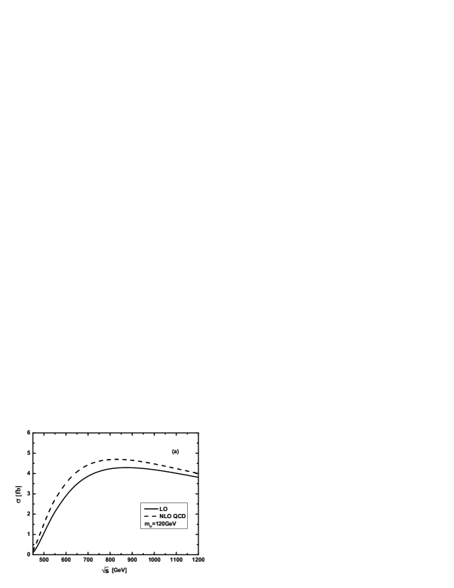
Figure 6: (a) The LO and QCD corrected cross sections for the process $e^{+}e^{-}\to t\bar{t}Z^{0}$ as the functions of colliding energy $\sqrt{s}$ with $m_{H}=120~{}GeV$. (b) The corresponding relative QCD radiative correction($\delta^{QCD}$) versus $\sqrt{s}$.

In Figs.7(a-b) we depict the curves of the LO cross section($\sigma_{0}$), ${\cal O}(\alpha_{ew})$ QED, weak, and total EW corrected cross sections($\sigma^{E,W,EW}\equiv\sigma_{0}+\Delta\sigma^{E,W,EW}$) as the functions of colliding energy $\sqrt{s}$ with $m_{H}=120~{}GeV$, and the corresponding relative radiative corrections($\delta^{E,W,EW}\equiv\frac{\Delta\sigma^{E,W,EW}}{\sigma_{0}}$) versus colliding energy are drawn in Fig.7(b). Figs.7(a-b) show that the QED and total EW corrections always suppress the LO cross section, while the weak correction part enhances the LO cross section, except it slightly suppresses the LO cross section in the region of $\sqrt{s}>1020~{}GeV$. The QED relative correction is about $-38.0\%$ at $t\bar{t}Z^{0}$ threshold and rises to $-2.8\%$ at $1.2~{}TeV$, but the weak relative correction is about $17.6\%$ at threshold and decreases to $-2.6\%$ at $1.2~{}TeV$. Thus the QED and weak contributions partially compensate each other when they combine to form the total EW correction, and yield the EW relative corrections of about $-20.4\%$ at threshold and $-5.4\%$ at $1.2~{}TeV$. Again, we see the Coulomb singularity effects on the curves of corrections $\delta^{E}$ and $\delta^{EW}$ in Fig.7(b) in the vicinity of threshold. There the curves for the QED, weak, and total EW relative corrections in Fig.7(b) demonstrate that the large EW corrections near the threshold region are mainly contributed by QED corrections which originate from the diagrams involving an instantaneous virtual photon in loop with a small spatial momentum. To show the numerical results presented in Figs.6(a-b) and Figs.7(a-b) more precisely, we list some typical numerical results for Born cross section($\sigma_{0}$), QCD, EW corrected cross sections($\sigma^{QCD}$, $\sigma^{EW}$) and QCD, EW relative corrections($\delta^{QCD,EW}\equiv\Delta\sigma^{QCD,EW}/\sigma_{0}$) for the process $e^{+}e^{-}\to t\bar{t}Z^{0}$ in Table 3. All these results show that when $\sqrt{s}$ goes up from $500~{}GeV$ to $1.2~{}TeV$, the relative QCD(EW) radiative correction, $\delta^{QCD}$($\delta^{EW}$), varies from $43.16\%$($-8.63\%$) to $4.99\%$($-5.42\%$).

Figure 7: (a) The LO cross section, QED, weak, and total EW corrected cross sections($\sigma^{E,W,EW}$) for the process $e^{+}e^{-}\to t\bar{t}Z^{0}$ as the functions of colliding energy $\sqrt{s}$ with $m_{H}=120~{}GeV$. (b) The corresponding relative QED, weak, and total EW radiative corrections ($\delta^{E,W,EW}$) versus $\sqrt{s}$.

$\sqrt{s}$ (GeV)	$\sigma_{0}(fb)$	$\sigma^{QCD}(fb)$	$\delta^{QCD}($%$)$	$\sigma^{EW}(fb)$	$\delta^{EW}($%$)$
500	1.0648(2)	1.5244(4)	43.16(3)	0.9729(6)	-8.63(5)
600	2.9432(4)	3.5741(7)	21.46(2)	2.805(2)	-4.70(7)
800	4.243(1)	4.698(2)	10.72(3)	4.070(4)	-4.07(7)
1000	4.187(1)	4.478(2)	6.93(4)	3.994(4)	-4.63(8)
1200	3.811(1)	4.001(2)	4.99(5)	3.604(4)	-5.42(8)

Table 3: The numerical results of the tree-level, one-loop QCD, EW corrected cross sections and the relative QCD, EW radiative corrections($\delta^{QCD,EW}\equiv\Delta\sigma^{QCD,EW}/\sigma_{0}$) for the process $e^{+}e^{-}\to t\bar{t}Z^{0}$ , by taking $m_{H}=120~{}GeV$ and $\sqrt{s}=500~{}GeV$, $600~{}GeV$, $800~{}GeV$, $1000~{}GeV$, $1200~{}GeV$, separately.

In Fig.8(a) we present the spectrums of the invariant mass of top-quark pair($M_{t\bar{t}}$) at LO, QCD(EW) one-loop order for the process $e^{+}e^{-}\to t\bar{t}Z^{0}$ by taking $m_{H}=120~{}GeV$ and $\sqrt{s}=500~{}GeV$. The distributions of the transverse momenta of top-quark($d\sigma_{0}/dp_{T}^{t}$, $d\sigma^{QCD,EW}/dp_{T}^{t}$) and $Z^{0}$-boson($d\sigma_{0}/dp_{T}^{Z}$, $d\sigma^{QCD,EW}/dp_{T}^{Z}$) are depicted in Fig.8(b) and (c), separately. Fig.8(a) shows that the QCD corrections always significantly enhance the LO differential cross section $d\sigma_{0}/dM_{t\bar{t}}$ in the whole plotted region, except the enhancement becomes much smaller when $M_{t\bar{t}}>400~{}GeV$, while the EW correction either slightly enhances the LO differential cross section of $d\sigma_{0}/dM_{t\bar{t}}$ in the region of $M_{t\bar{t}}<365~{}GeV$, or distinctly suppresses the differential cross section when $M_{t\bar{t}}>375~{}GeV$ as shown in Fig.8(a). All these three figures demonstrate that the QCD corrections induce the enhancement to the LO differential cross sections of the invariant mass of top-quark pair, the transverse momenta of top-quark and $Z^{0}$-boson. We can see from Figs.8(b) and (c) that the EW radiative corrections can only slightly reduce the LO differential cross sections of $d\sigma_{0}/dp_{T}^{t}$ and $d\sigma_{0}/dp_{T}^{Z}$ in all possible $p_{T}^{t}$ and $p_{T}^{Z}$ regions.

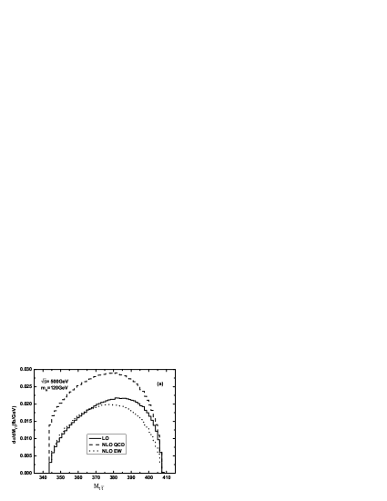
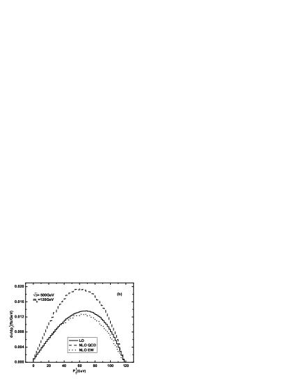
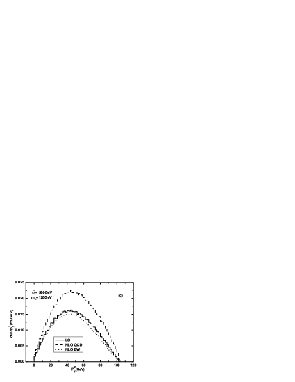
Figure 8: The spectrums for $e^{+}e^{-}\to t\bar{t}Z^{0}$ process at LO, QCD and EW one-loop order in conditions of $m_{H}=120~{}GeV$ and $\sqrt{s}=500~{}GeV$. (a) The spectrums of invariant mass of top-quark pair $M_{t\bar{t}}$. (b) The spectrums of the transverse momentum of top-quark $p_{T}^{t}$. (c) The spectrums of the transverse momentum of $Z^{0}$-boson $p_{T}^{Z}$.

VI. Summary

Probing precisely the top physics and searching for the signature of new physics are important tasks in present and future high energy physics experiments. The future $e^{+}e^{-}$ linear collider could provide much more efficient laboratory to put these measurements into practice with a cleanest environment. In this paper we have studied the full one-loop QCD and EW corrections to the $e^{+}e^{-}\to t\bar{t}Z^{0}$ process in the SM. We investigate the dependence of the effects coming from the QCD and EW contributions to the cross section of process $e^{+}e^{-}\to t\bar{t}Z^{0}$ on colliding energy $\sqrt{s}$. We find that the QCD correction enhances the tree-level cross section, while the one-loop EW correction suppresses the LO cross section. Our numerical results show that when $m_{H}=120~{}GeV$ and colliding energy has the values of $500~{}GeV$ and $1.2~{}TeV$, the corresponding relative QCD(EW) corrections are $43.16\%(-8.63\%)$ and $4.99\%(-5.42\%)$, respectively. We present also the LO, QCD and EW corrected differential cross sections of transverse momenta of final top-quark and $Z^{0}$-boson, and the distributions of top-quark pair invariant mass. We conclude that both the QCD and EW radiative corrections have relevant impact on the $e^{+}e^{-}\to t\bar{t}Z^{0}$ process, and should be included in any reliable analysis.

Acknowledgments: This work was supported in part by the National Natural Science Foundation of China(No.10575094), the National Science Fund for Fostering Talents in Basic Science(No.J0630319), Specialized Research Fund for the Doctoral Program of Higher Education(SRFDP)(No.20050358063) and a special fund sponsored by Chinese Academy of Sciences.

References

- [1] S. L. Glashow, Nucl. Phys. 22 (1961) 579; S. Weinberg, Phys. Rev. Lett. 1 (1967) 1264; A. Salam, Proc. 8th Nobel Symposium Stockholm 1968,ed. N. Svartholm (Almquist and Wiksells, Stockholm 1968) p.367; H. D. Politzer, Phys. Rep. 14 (1974) 129.
- [2] P. W. Higgs, Phys. Lett 12 (1964) 132, Phys. Rev. Lett. 13 (1964) 508; Phys. Rev. 145 (1966) 1156; F. Englert and R.Brout, Phys. Rev. Lett. 13 (1964) 321; G. S. Guralnik, C. R. Hagen and T. W. B. Kibble, Phys. Rev. Lett. 13 (1964) 585; T. W. B. Kibble, Phys. Rev. 155 (1967) 1554.
- [3] F. Abe, et al. (CDF Collaboration), Phys. Rev. Lett. 74, 2626 (1995).
- [4] S. Abachi, et al. (DØ Collaboration), Phys. Rev. Lett. 74, 2632 (1995).
- [5] D. Chakraborty, J. Konigsberg and D. Rainwater, Ann. Rev. Nucl. Part. Sci. 53, 301 (2003).
- [6] Tevatron Electroweak Working Group(for the CDF and D0 Collaborations), Fermilab-TM-2347-E, TEVEWWG/top 2006/01, CDF-8162, D0-5064, hep-ex/0603039v1.
- [7] W.M. Yao,et al. J. of Phys. G33,1 (2006).
- [8] C.F. Berger, M. Perelstein and F. Petriello, MADPH-05-1251, SLAC-PUB-11589, arXiv:hep-ph/0512053.
- [9] R.S. Chivukula, S.B. Selipsky and E.H. Simmons, Phys. Rev. Lett. 69, 575 (1992); R.S. Chivukula, E.H. Simmons and J. Terning, Phys. Lett. B331, 383 (1994); K. Hagiwara and N. Kitazawa, Phys. Rev. D52, 5374 (1995); U. Mahanta, Phys. Rev. D55, 5848 (1997) and Phys. Rev. D56, 402 (1997).
- [10] T. Abe et al. [American Linear Collider Working Group], in Proc of the APS/DPF/DPB Summer Study on the Future of Particle Physics(Snowmass 2001) ed. N. Graf, arXiv:hep-ex/0106057.
- [11] A. Djouadi, J.Ng, and T.G. Rizzo, SLAC-PUB-95-6772, GPP-UdeM-TH-95-17, TRI-PP-95-05, hep-ph/9504210; S.Y. Choi, and Hagiwara, Phys. Lett. B359,369(1005); M.S. Baek, S.Y. Choi, and C.S. Kim, Phys. Rev. D56,6835 (1997); P. Poulose and S.D. Rindani, Phys. Rev. D57,5444(1998); [61, 119902(E)(2002)]; Phys. Lett. B452,347(1999).
- [12] Hua Wang, Chong-Sheng Li, Hong-Yi Zhou, and Yu-Ping Kuang, Phys. Rev. D54 (1996) 4374.
- [13] Han Liang, Ma Wen-Gan, Yu Zeng-Hui, Phys. Rev. D56 (1997) 265.
- [14] Zhou Mian-Lai, Ma Wen-Gan, Han Liang, Jiang Yi, and Zhou Hong, Phys. Rev. D61, 033008(2000).
- [15] U. Baur, A. Juste, L.H. Orr, and D. Rainwater, Phys. Rev. D71, 054013 (2005).
- [16] K. Hagiwara, H. Murayama and I. Watanabe, Nucl. Phys. B367(1991), 257.
- [17] S. Bar-Shalom, D. Atwood, and A. Soni, Phys. LettB419(1998) 340.
- [18] B. Grzadkowski and J. Pliszka, Phys. Rev. D60(1999)115018.
- [19] A. Lazopoulos, T. McElmurry, K. Melnikov, F. Petriello, ’Next-to-leading order QCD corrections to production at the LHC’, UH-511-1125-08, arXiv:0804.2220v2[hep-ph]; A. Lazopoulos, K. Melnikov, F. Petriello, ’NLO QCD corrections to the production of in gluon fusion’, arXiv:0709.4044v1[hep-ph].
- [20] Parameters for Linear Collider, http://www.fnal.gov/directorate/icfa/LC_parameters.pdf
- [21] T. Hahn, Comput. Phys. Commun. 140 (2001)418.
- [22] A. Denner, Fortschr. Phys. 41, 307 (1993).
- [23] T. Hahn, M. Perez-Victoria, Comput. Phys. Commun. 118,(1999) 153; ”FormCalc5 User’s Guide”, http://www.feynarts.de/formcalc/.
- [24] G. J. van Oldenborgh, Phys Commun 66 (1991) 1, NIKHEF-H-90-15.
- [25] G.’t Hooft and M. Veltman, Nucl. Phys. B153, 365 (1979).
- [26] A. Denner and S. Dittmaier, Nucl. Phys. B658 (2003) 175.
- [27] E. Boos, V. Bunichev, et al., (the CompHEP collaboration), Nucl. Instrum. Meth. A534 (2004) 250-259, hep-ph/0403113.
- [28] G.P. Legage, J. Comput. Phys. 27, 192(1978); G.P. Legage,, VEGAS: An Adaptive Multidimensional Integration Program, Cornell University preprint CLNS-80/447(1980).
- [29] T. Kinoshita, J. Math. Phys. 3(1962) 650; T.D. Lee and M. Nauenberg, Phys. Rev. 133(1964) 1549.
- [30] B. W. Harris and J.F. Owens, Phys. Rev. D65 (2002) 094032, arXiv:hep-ph/0102128.
- [31] W. T. Giele and E. W. N. Glover, Phys. Rev. D46, 1980 (1992); W. T. Giele, E. W. Glover and D. A. Kosower, Nucl. Phys. B403, 633 (1993); S. Keller and E. Laenen, Phys. Rev. D59, 114004 (1999).
- [32] S. Dawson and L. Reina, Phys. Rev. D59, 054012 (1999),arXiv:hep-ph/9808443.
- [33] F. Legerlehner, DESY 01-029, arXiv:hep-ph/0105283.
- [34] R. Barate et al., Phys. Lett. B565 (2003) 61.
- [35] The LEP Collaborations ALEPH, DELPHI, L3, OPAL, and the LEP Electroweak Working Group. LEPEWWG/2007-01 and arxiv:0712.0929.
- [36] T. Ishikawa,et al., (MINMI-TATEYA collaboration) ”GRACE User’s manual version 2.0”, August 1, 1994.
- [37] A. Denner, U Nierste and R Scharf, Nucl. Phys. B367 (1991) 637.