The luminosity function of galaxies to $M_{BgVriz}\sim-14$ in $z\sim 0.3$ clusters

Abstract

We present deep composite luminosity functions in $B$, $g$, $V$, $r$, $i$ and $z$ for six clusters at $0.14<z<0.40$ observed with the Hubble Space Telescope Advanced Camera for Surveys. The luminosity functions reach to absolute magnitude of $\sim-14+5\log h$ mag. and are well fitted by a single Schechter function with $M^{*}_{BgVriz}=-19.8,\,-20.9\,-21.9,\,-22.0,\,-21.7,\,-22.3$ mag. and $\alpha\sim-1.3$ (in all bands). The observations suggest that the galaxy luminosity function is dominated by objects on the red sequence to at least 6 mags. below the $L^{*}$ point. Comparison with local data shows that the red sequence is well established at least at $z\sim 0.3$ down to $\sim 1/600^{th}$ of the luminosity of the Milky Way and that galaxies down to the regime of dwarf spheroidals have been completely assembled in clusters at this redshift. We do not detect a steepening of the luminosity function at $M>-16$ as is observed locally. If the faint end upturn is real, the steepening of the luminosity function must be due to a newly infalling population of faint dwarf galaxies.

1 Introduction

The galaxy luminosity function (hereafter LF) provides a $0^{th}$ order description of the gross properties of galaxy populations. Although it may be regarded as somewhat simplistic, in reducing galaxy properties to the two numbers ($M^{*}$ and $\alpha$) that describe the LF in the Schechter (1976) form, reproducing the observed LF is a fundamental test for any viable theory of galaxy formation, and one that has proven surprisingly complex to achieve until relatively recently (e.g., Croton et al. 2006).

Clusters of galaxies are, in several ways, ideal laboratories to study the LF and its evolution. Cluster galaxies may be considered as a volume limited sample of objects observed at the same cosmic epoch and occupy a relatively ‘constant’ environment corresponding to the highest density peaks at the redshift of observation. Operationally, cluster members have a much higher surface density on the sky than the surrounding field and often exhibit distinctive morphologies and colors (see Fig. 1 below). It is therefore possible to establish membership in a cluster (at least in a statistical sense) without resorting to observationally expensive redshift surveys.

On the other hand, clusters are obviously special places, containing only a small percentage ($5$–$10\%$) of all galaxies in the Universe. Their galaxy populations clearly implicate the cluster environment in a variety of processes that affect the morphological evolution of galaxies (e.g., Dressler 1980) and suppress or modify their star formation history (Lewis et al., 2002; Gomez et al., 2003). In order to use clusters as probes of galaxy evolution it is therefore important to understand the effects of environment and carry out careful comparisons with field samples. For local samples, this is now possible thanks to large redshift surveys such as 2dF (Colless et al., 2001) and SDSS (York et al., 2000).

Although bright galaxies appear to have formed the majority of their stellar populations and assembled their mass at least by $z=1.5$ (e.g., Andreon 2006a; De Propris et al. 2007; Muzzin et al. 2008 and references therein), there is considerable evidence that fainter galaxies undergo significant evolution since $z=1$. The red sequence in clusters in the EDisCS sample appears to be truncated at faint magnitudes (De Lucia et al., 2007), while Stott et al. (2007) show that the luminosity function of red cluster galaxies flattens at higher redshifts, as do Krick et al. (2008) for clusters in a deep Spitzer field. On the other hand, there are clusters with well-formed red sequences at redshifts approaching $1$ as well (Andreon, 2006b; Crawford et al., 2008). It may not be surprising that the faint end of the LF shows considerable variations from cluster to cluster, as one expects that dwarfs are more sensitive to environmental effects. Although the bright end of the LF ($M<-16$) is broadly universal, the faint end varies between clusters and may even change radially within clusters (Popesso et al., 2006; Barkhouse et al., 2007).

The evolution of the faint end slope of the total LF provides an interesting test of galaxy formation models. Even if the red sequence is truncated at faint luminosities at earlier epochs, one expects a steepening faint end as established by the initial power spectrum of fluctuations, which is very steep (Khochfar et al., 2007). In higher redshift clusters, there should be a steeper LF and a larger fraction of bluer dwarfs.

The purpose of this paper is to explore the evolution of the LF to very faint magnitudes in a sample of $z\sim 0.3$ clusters observed with the Hubble Space Telescope (HST), reaching well below the $L^{*}$ point and into the domain of dwarf spheroidal galaxies, using a multicolor imaging sample. This will allow to test scenarios for the evolution of dwarf galaxy populations in $\Lambda$CDM hierarchical models. The structure of this paper is as follows: we describe the data and photometry in the next section. We derive the composite LFs and then discuss the results in the context of galaxy formation models. We adopt the ‘consensus’ cosmology with $\Omega_{M}=0.27$, $\Omega_{\Lambda}=0.73$ and use H₀=100 km s^-1 Mpc^-1. All data are photometrically calibrated to the AB system, using the latest ACS zeropoints published on the HST Instrument Web page.

2 Observations and Data Analysis

Observations for this paper consist of deep HST imaging of six clusters at $0.14<z<0.40$ taken with the Advanced Camera for Surveys (ACS) in the $B$ (F435W), $g$ (F475W), $V$ (F555W), $r$ (F625W), $i$ (F775W) and $z$ (F850LP) bands with exposure times of 5,000–10,000 seconds in each band. Each cluster was observed in a single ACS exposure, covering about $200^{\prime\prime}$ on the sky. The data were originally taken for studies of gravitational lenses in these clusters. Table 1 shows the clusters observed, their redshifts, exposure times in each band, and HST proposal IDs. Table 2 summarizes some essential physical characteristics for the observed clusters. Most data are from the compilation of Wu et al. (1999), from which $r_{200}$ can be estimated via the formula of Carlberg et al. (1997), except for A1413 where $r_{200}$ was derived by Pointecouteau et al. (2005) from the X-ray profile. We were unable to find data in the literature for A1703.

The data were retrieved from the HST archive as fully reduced and flatfielded files (*.flt) and then processed through the Multidrizzle algorithm (Koekemoer et al., 2002) to produce fully registered and co-added images for each band. Fig. 1 shows color composites for our data. Full resolution JPEGs will be made available on the $AJ$ web site.

Detection of objects and photometry were carried out using Sextractor (Bertin & Arnouts, 1996). We experimented with Sextractor parameters to maximize our detections and minimize the number of spurious objects. All detections were visually examined to eliminate noise spikes, bleed trails from bright stars and other contaminants, especially the numerous arclets present in the images. The Sextractor parameters eventually employed are shown in Table 3. We used the same parameters for all images.

For each object we compute a total (Kron-like) magnitude and an aperture magnitude of area equivalent to the minimum number of connected pixels needed for detection. This provides an estimate of the central surface brightness for each object. The motivation behind this procedure is as follows. Detections of objects in deep images depends on their total magnitude but also on their central surface brightness. An object could be brighter than the magnitude threshold but be lost in the night sky because of low surface brightness (see discussion in Cross & Driver 2002). For this reason we need to determine both a limiting total magnitude for completeness and a surface brightness threshold for detection.

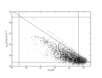
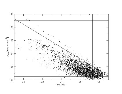
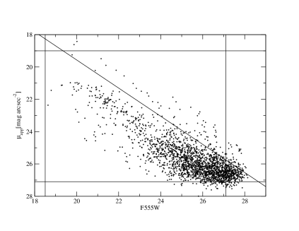
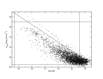
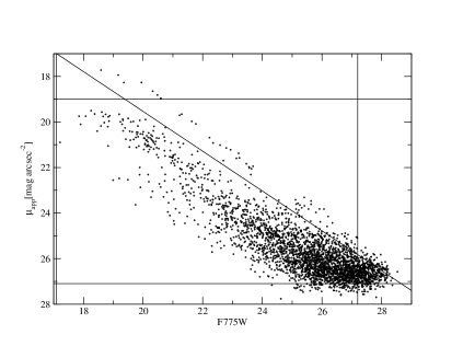
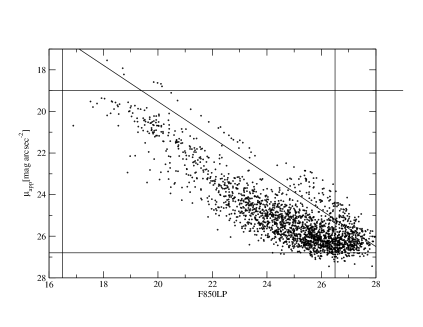
Figure 2: Mean central surface brightness vs. total magnitudes for objects in the Abell 1703 field. Selection lines show the star-galaxy separation, the surface brightness threshold and the magnitude completeness limit. Similar figures for all the other objects in our sample can be found in the electronic version of this paper.

We do this by plotting central surface brightness vs. total magnitude for all bands in Fig. 2. To save space we only show the data for Abell 1703, but equivalent figures for all other clusters are available on the $AJ$ web site. In these figures the sequence at high surface brightness that provides an upper limit to the scatter plot is caused by stars. We can therefore discriminate against stellar contamination in this way (cf. Garilli et al. 1999). The surface brightness threshold is chosen empirically. The limit is selected to include as many objects as possible, but avoiding regions of the parameter space where the sample is obviously very incomplete. Selection lines in surface brightness, apparent magnitude and the star-galaxy separation line are shown in Fig. 2.

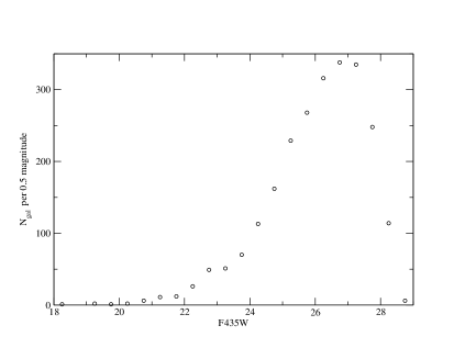
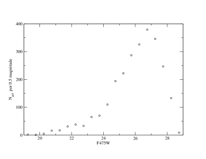
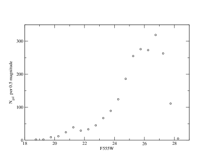
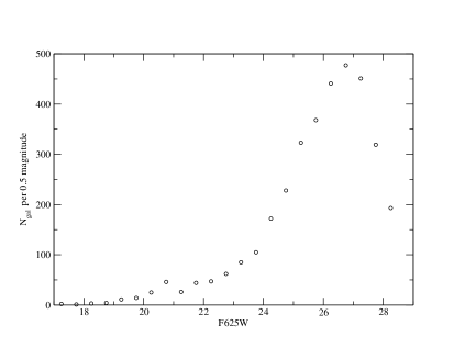
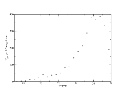
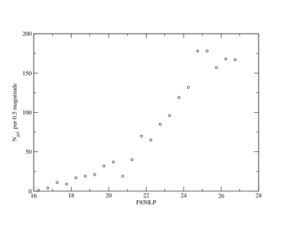
Figure 3: Raw galaxy number counts in the Abell 1703 field. See the electronic version of this paper for the relative figures for all other targets.

In order to determine a limiting magnitude, we plot the raw number counts for galaxies in the Abell 1703 field in Fig. 3. As for Fig. 2, figures for all the other clusters are made available electronically. The completeness magnitude is chosen to lie about 0.5 mag. brighter than the luminosity at which counts start to decrease, in order to select a highly complete sample of objects.

The only way to establish cluster membership for faint galaxies is by statistical background subtraction. In order to do so, we need to analyze ‘blank’ (cluster-less) comparison fields of similar or greater photometric depth. We choose to use the two GOODS fields (Giavalisco et al., 2004) as these are the deepest and widest fields where HST multicolor photometry is available.

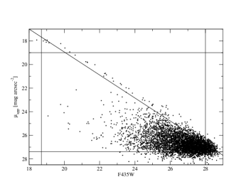
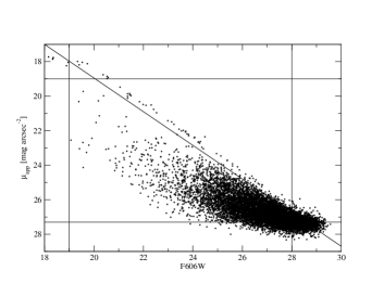
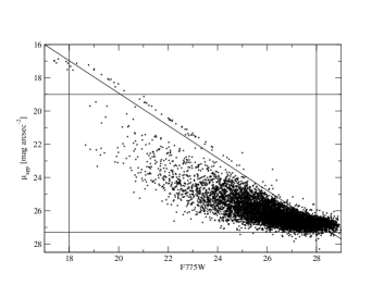
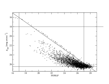
Figure 4: Same as Fig. 2, but for the combined GOODS fields. We only plot a random selection of 10% of the objects in the GOODS fields, for clarity.

We used the same Sextractor parameters as we used for the cluster fields and impose the same selection limits on the GOODS fields as we did for the target fields. Fig. 4 shows the detection and selection plots for the GOODS fields (similar to Fig. 2 above). The fields are much deeper than the cluster fields we use. It must be noted that we plot only $10\%$ of the detections in the GOODS fields in Fig. 4 to avoid saturating the figure.

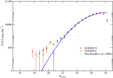
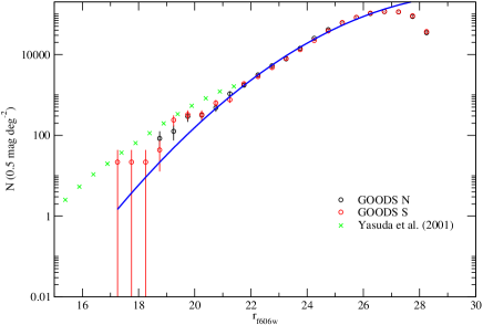
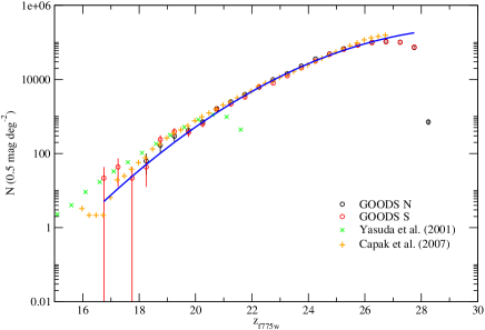
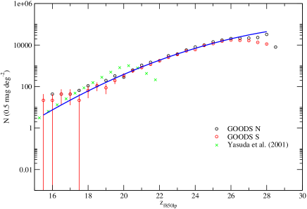
Figure 5: Number counts for the GOODS fields and quadratic fits. Literature counts (see text) are also shown.

Fig. 5 plots galaxy number counts for the GOODS fields and comparison galaxy number counts from the literature. The HST data were corrected to the SDSS and Johnson-Cousins systems using the transformations tabulated in Holberg & Bergeron (2006). GOODS number counts were fitted with a quadratic of the form $a_{0}+a_{1}x+a_{2}x^{2}$. The fit was carried out over galaxies brighter than the completeness limit shown in Fig. 4 and fainter than m$\sim 21$ mag. as GOODS counts for brighter galaxies are affected by small scale clustering. Table 4 shows the values of the coefficients for the quadratic fits.

3 Luminosity Functions

We now subtract the scaled contribution from fore/background counts from galaxy counts. Errors in galaxy counts for clusters and the GOODS fields are assumed to be Poissonian. We used our smoothed quadratic for the background counts, extrapolating for galaxies brighter than $m\sim 21$ mag. Field counts at these bright limits and over the small ($\sim 9$ arcmin²) covered by ACS are very small in any case. Clustering errors over the cluster and GOODS fields are estimated following the counts-in-cells approach and the fitting formula described by Huang et al. (1997).

It may be possible to further refine the selection of cluster members using photometric redshifts or color cuts. Contamination of the LF by background galaxies has been suggested as a possible cause of the faint end upturn (see below) by Valotto et al. (2001). However, this would lead to loss of generality. The argument by Valotto et al. (2001) may be correct for nearby clusters (although Andreon et al. 2005 point out that the simulations used by Valotto et al. 2001 are unrealistic and that the background subtraction approach used here works as long as proper care is taken of statistical uncertainties, see their §3.3.6), but it is not appropriate for these distant objects where the redshift is much larger than the typical scale of structure in the Universe (so that the counts should be smooth).

There are some mismatches between the GOODS data (used for background subtraction) and the cluster data. For the $g$ (F435W) and $r$ (F625W) bands, we can use the GOODS F475W and F606W counts (respectively), which are close matches to the bands used, however, for F555W ($V$) we used the average of the F475W and F606W counts. The LF in this bands is more uncertain, because we do not have an appropriate background field.

We $k$ and $e$ correct the LFs to $z=0$ for ease of comparison with local data. In order to do so we use a Bruzual & Charlot (2003) model for a solar metallicity elliptical formed at $z=3$ with an e-folding time of 1 Gyr. This is appropriate to the red ellipticals that dominate the bright end of cluster LFs. In effect this approach allows us to consider the differential evolution, if any, between the dwarfs and the giants, who appear to consist mainly of old galaxies with little or no recent star formation.

The LF of each individual cluster is relatively uncertain. We therefore build composite LFs in each band following the method by Colless (1989) in order to average out errors. The method assumes that the LF is broadly universal, but this appears to be borne out by observations at low redshift, at least for relatively bright galaxies (Popesso et al., 2006; Barkhouse et al., 2007).

Composite LFs are built as follows: the number of cluster galaxies in the $j^{th}$ magnitude bin of the composite LF is given by:

$$N_{cj}={N_{c0}\over m_{j}}{\sum_{i}{N_{ij}\over N_{i0}}}$$ (1)

where $N_{ij}$ is the (background corrected) number of galaxies in the $j^{th}$ magnitude bin of the LF of the $i^{th}$ cluster LF, $N_{i0}$ is the normalization of the cluster LF (to take care of the different richnesses of the clusters) and is taken to be the background corrected number of cluster galaxies brighter than $M_{B}=-19$ (or its equivalent in the other bands, assuming the color of an old elliptical), $m_{j}$ is the number of $i$ clusters contributing to the $j^{th}$ magnitude bin of the composite LF and $N_{c0}$ is the sum of all the $i$ normalizations.

$$N_{c0}=\sum_{i}N_{i0}$$ (2)

Essentially, this carried out a weighted average of the individual cluster LFs, scaled by the number of galaxies (in each cluster) brighter than approximately the $L^{*}$ point. The formal errors on $N_{cj}$ are computed as:

$$\delta N_{cj}={N_{c0}\over m_{j}}\left[\sum_{i}\left({\delta N_{ij}\over N_{i0}}\right)^{2}\right]^{1/2}$$ (3)

where $\delta N_{ij}$ are the errors on the number counts (including Poissonian and clustering contributions) for the $j^{th}$ magnitude bin of the $i^{th}$ cluster LF.

For each cluster we build the composite LF by summing up the individual LFs in absolute magnitude bins, after correcting for the distance modulus, extinction and $k+e$ correction to the common redshift of $z=0$.

The resulting LFs are presented in Fig. 6, together with the 1, 2 and 3$\sigma$ error countours. We fit the data to a single Schechter function (see discussion below, regarding the existence of a faint end upturn). In some cases we exclude the fainter and/or brighter magnitude bin from the fit, because these points are dominated by either the poorly sampled very massive galaxies or the fainter objects that suffer from complex incompleteness due to magnitude and surface brightness selection. The fit parameters are tabulated in Table 5, together with the $1\sigma$ errors for each parameter, marginalized over the remaining parameters.

4 Discussion

There are only a few deep cluster LFs having comparable depth to our own. In general, we are in good agreement with previous work, based on smaller and shallower samples (Driver et al., 1994; Trentham, 1998a; Boyce et al., 2001; Mercurio et al., 2003; Pracy et al., 2004; Andreon et al., 2005; Harsono & De Propris, 2007). The $M^{*}$ point we measure gets steadily brighter with increasing wavelength, tracking the color of old, passively evolving stellar populations that are the main component of bright elliptical galaxies (Cool et al., 2006). The value we find is also consistent with the local SDSS value by Popesso et al. (2006): this is not surprising, as it is well known that massive galaxies evolve passively since high redshift.

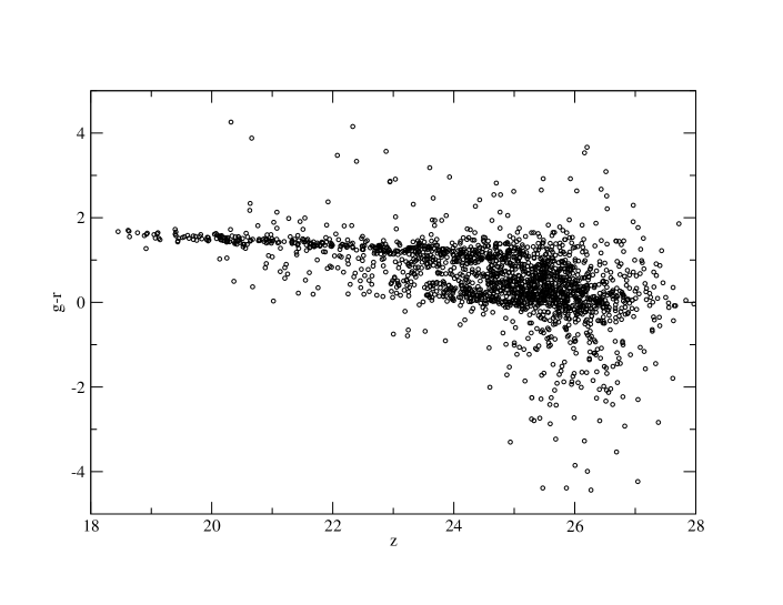
Figure 7: The color magnitude diagram for galaxies in A1703

The main interest of this investigation is in the evolution of the LF slope. The LF is well fitted by a single Schechter function, with a slope $\alpha\sim-1.3$ which is essentially the same in all bands. This suggests that the cluster LF is dominated by galaxies on the red sequence to a luminosity of $M\sim-14$ in all bands, and that therefore the red sequence continues at least to 6 magnitudes below the $L^{*}$ point even at $z\sim 0.3$. This can be clearly seen in Fig. 7 where we show the $g-r$ vs. $z$ color-magnitude relation for Abell 1703. The relation can be clearly followed at least to $z=25$ with little scatter. A more detailed analysis of the color-magnitude relation is deferred to a future paper (Harsono & De Propris 2008, in preparation). The red sequence appears to be well established and contain the majority of cluster populations even at a lookback time of $\sim 3.5$ Gyrs (cf. Andreon et al. 2006; Eisenhardt et al. 2007 for a similarly deep relation in local clusters).

The slope is very similar to the local value for $M<-16$ derived by Popesso et al. (2006) and Barkhouse et al. (2007). This argues that even galaxies to $M\sim-14$ have formed their stellar populations and assembled the majority of their mass at least at $z\sim 0.3$. We can therefore place a significant lower limit to the assembly epoch of galaxies down to 1/600^th of the mass of the Milky Way. Given the evidence for truncation of the red sequence at $z\sim 0.8$ (De Lucia et al., 2007; Stott et al., 2007; Krick et al., 2008), our data point to the $0.3<z<0.8$ interval as a crucial epoch to investigate the formation of the fainter galaxy populations.

The other issue we wish to address is the faint end upturn. This has been a controversial subject, ever since its original discovery by Driver et al. (1994) and De Propris et al. (1995). There have been a series of claims and counterclaims regarding the faint end slope and the existence of an upward inflection, sometimes even in the same cluster. For instance, De Propris et al. (1998); Trentham (1998b); Adami et al. (2007); Jenkins et al. (2007) and Milne et al. (2007) observe a steep LF at the faint end for the Coma cluster, while Bernstein et al. (1995); Adami et al. (1998) and Beijersbergen et al. (2002) quote much flatter slopes. In Virgo, Sabatini et al. (2005) claim a slope as steep as $\sim-1.6$, while Rines & Geller (2008) derive $\alpha=-1.3$. Baldry et al. (2008) review the existence of the upturn and the shape of the faint end of the LF and conclude that there is a steep mass function. The observation of the upturn in two composite LFs, derived by two different groups (Popesso et al., 2006; Barkhouse et al., 2007), suggests that the upward inflection of the LF is real (however, cf., Hilker et al. 2003; Penny & Conselice 2008).

Unlike Popesso et al. (2006) and Barkhouse et al. (2007) we do not find a steepening of the LF at $M>-16$. However, we must consider that the LF upturn is more pronounced at large clustercentric radii, while our fields generally cover only the central region of each cluster. The size of the ACS fields used in this study covers between 350 and 750 $h^{-1}$ kpc on the side. In terms of $R_{200}$ (the radius at which Popesso et al. 2006 and Barkhouse et al. (2007) normalize their LFs), the areas imaged by ACS cover between 20% and 40% of the area of the cluster out to $r_{200}$. We therefore only derive LFs for the cluster cores. This should not affect our comparisons with the bright end of the LF ($M<-16$), as this does not seem to vary significantly with radius. However, the steep upturn claimed by Popesso et al. (2006) and Barkhouse et al. (2007) is much more pronounced at large clustercentric radii, i.e., in the cluster outskirts. On the other hand it is possible to see the upturn even in the more central regions of the sample studied by Popesso et al. (2006), inside $\sim 0.3r_{200}$ (see Fig. 10 of Popesso et al. 2006), so our data should exhibit an upturn at faint magnitudes, although of course more clusters would be welcome to bolster the argument.

As we do not detect a steepening in the LF, we suggest that, if the steepening is real, the faint galaxies contributing to the upturn consist of a population of recently infalling objects (e.g., Smith et al. 2008) whose star formation is curtailed by the cluster environment. This would be consistent with the observation that about 1/2 of the fainter cluster dwarfs in Virgo and elsewhere have been forming stars until relatively recently (Conselice et al., 2001, 2003), until their star formation stopped and their colors moved to the red sequence. The newly infalling population may be the one now contributing to the steep upturn. In a ‘downsizing’ model, it may be expected that objects undergoing star formation suppression and cluster infall at the present epoch would indeed tend to be among the fainter and less massive galaxies and to have the steep LF characteristic of ‘pristine’ CDM power spectra.

Our observations imply that the passive evolution of bright galaxies can be extended to faint dwarfs, at least to $z\sim 0.3$ and suggest that the majority of galaxy evolution may have taken place at surprisingly early epochs even for the least massive objects.

Figure 1: Colour images of target clusters. From left to right: A1413, A1689, A2218, A1703, MS1358 and Cl0024. These figures exceed arXiv size limits and cannot be compressed further. They will appear as JPEG in AJ. Please email rdepropris@ctio.noao.edu for the figures to be sent to you via FTP (provide site) or email

Figure 6: Composite luminosity functions, best fits and error ellipses for the $B$ and $g$ bands

Figure 6: (Continued): for the $V$ and $r$ bands

Figure 6: (Continued): for the $i$ and $z$ bands

Table 1: Archival HST cluster observations

Cluster	redshift	$B$ Exposure	$g$	$V$	$r$	$i$	$z$	Proposal ID
Abell 1413	0.143	$\cdots$	$\cdots$	$\cdots$	$\cdots$	2440	2560	9292
Abell 2218	0.171	7048	5640	7048	8386	10732	5640	9452, 9717, 10325
Abell 1689	0.183	$\cdots$	9500	$\cdots$	9500	11800	16600	9289
Abell 1703	0.258	7050	5564	5564	9834	11128	17800	10325
MS 1358.4+6245	0.328	7928	5470	5482	9196	10952	15017	9292, 9717, 10325
Cl 0024.0+1652	0.395	6435	5072	5072	8971	10144	16328	10325

Table 2: Cluster properties

Cluster	redshift	$\sigma$ [km s-1]	$T$ (KeV)	$L_{X}$ ($10^{44}$ [ergs s-1]	$r_{200}$ (Mpc $h^{-1}$)	Coverage (% $r_{200}$)
Abell 1413	0.143	$\cdots$	$8.85\pm 0.50$	$36.01\pm 4.54$	1.71	21
Abell 2218	0.171	$1800\pm 207$	$9.02^{+0.40}_{-0.30}$	$55.73\pm 8.92$	2.94	14
Abell 1689	0.183	$1370^{+180}_{-220}$	$7.10\pm 0.20$	$21.96\pm 2.01$	2.24	19
Abell 1703	0.258	$\cdots$	$\cdots$	$\cdots$	$\cdots$	$\cdots$
MS 1358.4+6245	0.328	$937\pm 54$	$7.50\pm 4.30$	$21.81\pm 3.81$	2.40	28
Cl 0024.0+1652	0.395	$1339\pm 233$	$\cdots$	$4.26\pm 0.01$	1.95	39

Table 3: Sextractor parameters

Parameter	Value
DETECT MINAREA	7.0 pixels
DETECT THRESH	2.0
ANALYSIS THRESH	2.0
DEBLEND NTHRESH	32
PHOT APERTURES	1.5
PHOT AUTOPARAMS	2.5, 3.5

Table 4: Quadratic fits to GOODS counts

Band	a0	a1	a2
$g$ (F475W)	$-44.46$	3.544	$-0.06346$
$r$ (F606W)	$-23.58$	1.928	$-0.03196$
$i$ (F775W)	$-18.51$	1.590	$-0.02643$
$z$ (F850LP)	$-10.50$	0.9377	$-0.01417$

Table 5: Best fit parameters for composite LFs

Band	$M^{*}$	$\alpha$	$\chi^{2}_{\nu}$
$B$ (F435W)	$-19.80\pm 0.27$	$-1.29\pm 0.06$	$0.59$
$g$ (F475W)	$-20.94\pm 0.17$	$-1.31\pm 0.04$	$0.95$
$V$ (F555W)	$-21.86\pm 0.27$	$-1.27\pm 0.05$	$1.08$
$r$ (F625W)	$-21.95\pm 0.29$	$-1.33\pm 0.03$	$0.43$
$i$ (F775W)	$-21.66\pm 0.27$	$-1.27\pm 0.04$	$0.37$
$z$ (F850LP)	$-22.26\pm 0.30$	$-1.45\pm 0.02$	$0.94$

References

- Adami et al. (1998) Adami, C., Nichol, R. C., Mazure, A., Durret, F., Holden, B. & Lobo, C. 1998, A&A, 334, 765
- Adami et al. (2007) Adami, C., Picat, J. P., Durret, F., Mazure, A., Pelló, R. & West, M. 2007, A&A, 472, 749
- Andreon et al. (2005) Andreon, S., Punzi, G., Grado, A. 2005, MNRAS, 360, 727
- Andreon (2006a) Andreon, S. 2006a, A&A, 448, 447
- Andreon (2006b) Andreon, S. 2006b, MNRAS, 369, 969
- Andreon et al. (2006) Andreon, S., Cuillandre, J.-C., Puddu, E. & Mellier, Y. 2006, MNRAS, 372, 60
- Baldry et al. (2008) Baldry, I. K., Glazebrook, K. & Driver, S. P. 2008, MNRAS, 388, 945
- Barkhouse et al. (2007) Barkhouse, W. A., Yee, H. K. C. & Lopez-Cruz O. 2007, ApJ, 671, 1471
- Beijersbergen et al. (2002) Beijersbergen, M., Hoekstra, H., van Dokkum, P. G.& van der Hulst, T. 2002, MNRAS, 329, 385
- Bernstein et al. (1995) Bernstein, G. M., Nichol, R. C., Tyson, J. A., Ulmer, M. P. & Wittman, D. 1995, AJ, 110, 1507
- Bertin & Arnouts (1996) Bertin E., Arnouts S. 1996, A&AS, 117, 393
- Boyce et al. (2001) Boyce, P. J., Phillipps, S., Jones, J. B., Driver, S. P., Smith, R. M., & Couch, W. J. 2001, MNRAS, 328, 277
- Bruzual & Charlot (2003) Bruzual, G. & Charlot, S. 2003, MNRAS, 344, 1000
- Capak et al. (2007) Capak, P. et al. 2007, ApJS, 172, 99
- Carlberg et al. (1997) Carlberg, R. G., Yee, H. K. C. & Ellingson, E. 1997, ApJ, 478, 462
- Crawford et al. (2008) Crawford, S. M., Bershady, J. A. & Hoessel, J. G. 2008, astro.ph 0809.1661
- Colless (1989) Colless, M. M. 1989, MNRAS, 237, 799
- Colless et al. (2001) Colless, M. M. et al. 2001, MNRAS, 328, 1039
- Conselice et al. (2001) Conselice, C. J., Gallagher, J. S. & Wyse, R. F. G. 2001, ApJ, 559. 791
- Conselice et al. (2003) Conselice, C. J., Gallagher, J. S. & Wyse, R. F. G. 2003, AJ, 125, 66
- Cool et al. (2006) Cool, R. J., Eisenstein, D. J., Scranton, R., Brinkmann, J., Schneider, D. P. & Zehavi, I. 2006, AJ, 131, 736
- Cross & Driver (2002) Cross, N. J. G. & Driver, S. P. 2002, MNRAS, 329, 579
- Croton et al. (2006) Croton, D. et al. 2006, MNRAS, 365, 11
- De Lucia et al. (2007) De Lucia, G. et al. 2007, MNRAS, 374, 809
- De Propris et al. (1995) De Propris, R., Pritchet, C. J., Hartwick, F. D. A. & McClure, R. D. 1995, ApJ, 450, 534
- De Propris et al. (1998) De Propris, R., Eisenhardt, P. R., Stanford, S. A. & Dickinson, M. 1998, ApJ, 503, L45
- De Propris et al. (2007) De Propris, R., Stanford, S. A., Eisenhardt, P. R., Holden, B. P. & Rosati, P. 2007, AJ, 133, 2207
- Dressler (1980) Dressler, A. 1980, ApJ, 236, 351
- Driver et al. (1994) Driver, S. P., Phillipps, S., Davies, J. I., Morgan, I., Disney, M. J. 1994, MNRAS, 268, 393
- Eisenhardt et al. (2007) Eisenhardt, P. R., De Propris, R., Gonzalez, A. H., Stanford, S. A., Wang, M. & Dickinson, M. 2007, ApJS, 169, 225
- Garilli et al. (1999) Garilli, B., Maccagni, D. & Andreon, S. 1999, A&A, 353, 479
- Giavalisco et al. (2004) Giavalisco, M. et al. 2004, ApJ, 600, L93
- Gomez et al. (2003) Gomez, P. L. et al. 2003, ApJ, 584, 210
- Harsono & De Propris (2007) Harsono D. & De Propris R. 2007, MNRAS, 380, 1036
- Hilker et al. (2003) Hilker, M., Mieske, S. & Infante, L. 2003, A&A, 397, L9
- Holberg & Bergeron (2006) Holberg, J. B. & Bergeron P. 2006, AJ, 132, 1221
- Huang et al. (1997) Huang J.-S., Cowie L. L., Gardner J. P., Hu E. M., Songaila A., Wainscoat R. J. 1997, ApJ, 476, 12
- Jenkins et al. (2007) Jenkins, L. P., Hornschemeier, A. E., Mobasher, B., Alexander, D. M. & Bauer, F. E. 2007, ApJ, 666, 846
- Koekemoer et al. (2002) Koekemoer, A., Fruchter, A. S., Hook, R. N. & Hack, W. 2002, in The 2002 HST Calibration Workshop: Hubble after the installation of ACS and the NICMOS cooling system ed. by S. Arribas, A. Koekemoer, B. Whitmore (Baltimore: Space Telescope Science Institute), p. 337
- Khochfar et al. (2007) Khochfar, S., Silk, J., Windhorst, R. A. & Ryan, R. E. 2007, ApJ, 668, L115
- Krick et al. (2008) Krick, J. E., Surace, J. A., Thompson, D., Ashby, M. L. N., Hora, J. L., Gorjian, V. & Yan, L. 2008, astro-ph 0807.1565
- Lewis et al. (2002) Lewis, I. J. et al. 2002, MNRAS, 334, 673
- MacDonald et al. (2004) MacDonald, E. C. et al. 2004, MNRAS, 352, 1255
- Mercurio et al. (2003) Mercurio, A., Massarotti, M., Merluzzi, P., Girardi, M., La Barbera, F. & Busarello, G. 2003, MNRAS, 408, 57
- Milne et al. (2007) Milne, M. L., Pritchet, C. J., Poole, G. B., Gwyn, S. D. J., Kavelaars, J. J., Harris, W. E. & Hanes, D. A. 2007, AJ, 133, 177
- Muzzin et al. (2008) Muzzin, A., Wilson, G., Lacy, M., Yee, H. K. C. & Stanford, S. A. 2008, astro-ph 0807.0227
- Penny & Conselice (2008) Penny, S. J. & Conselice, C. J. 2008, MNRAS, 383, 247
- Pointecouteau et al. (2005) Pointecouteau, E., Arnaud, M. & Pratt, G. W. 2005, A&A, 435, 1
- Popesso et al. (2006) Popesso, P., Biviano, A., Böhringer, H. & Romaniello, M. 2006, A&A, 445, 29
- Pracy et al. (2004) Pracy, M., De Propris, R., Driver, S. P., Couch, W. J. & Nulsen, P. E. J. 2004, MNRAS, 352, 1135
- Rines & Geller (2008) Rines, K. & Geller, M. J. 2008, AJ, 135, 1837
- Sabatini et al. (2005) Sabatini, S., Davies, J. I., Scaramella, R., Smith, R., Baes, M., Linder, S. M., Roberts, S. & Testa, M. 2005, MNRAS, 357, 819
- Schechter (1976) Schechter, P. 1976, ApJ, 203, 297
- Smith et al. (2008) Smith, R. J. et al. 2008, MNRAS, 386, L96
- Stott et al. (2007) Stott, J. P., Smail, I., Edge, A. C., Ebeling, H., Smith, G. P., Kneib, J.-P. & Pimbblet, K. A. 2007, ApJ, 661, 95
- Trentham (1998a) Trentham, N. 1998a, MNRAS, 295, 360
- Trentham (1998b) Trentham, N. 1998b, MNRAS, 293, 71
- Valotto et al. (2001) Valotto, C., Moore, B. & Lambas, D. G. 2001, ApJ, 546, 157
- Wright (2006) Wright, E. L. 2006, PASP, 118, 1711
- Wu et al. (1999) Wu, X.-P., Xue, Y.-J. & Fang, L.-Z. 1999, ApJ, 524, 22
- Yasuda et al. (2001) Yasuda, N. et al. 2001, AJ, 122, 1104
- York et al. (2000) York, D. G. et al. 2000, AJ, 120, 1579