Dissecting the Red Sequence—I. Star Formation Histories of Quiescent Galaxies: The Color-Magnitude vs. the Color-$\sigma$ Relation

Abstract

We use a sample of $\sim$16,000 non-emission line galaxies from the SDSS to investigate the physical parameters underlying the well-known color-magnitude and color-$\sigma$ relations. Galaxies are sorted in terms of velocity dispersions ($\sigma$), luminosity ($L$), and color, and their spectra are stacked to obtain very high $S/N$ mean spectra for stellar population analysis. This allows us to map mean luminosity-weighted ages, [Fe/H], [Mg/H], and [Mg/Fe] in $\sigma$-$L$-color space. Our first result is that there are many different red sequences, with age, [Fe/H], [Mg/H], and [Mg/Fe] showing different amounts of slope and scatter when plotted versus $\sigma$, $L$, or color. These behaviors are explained if the star formation histories of the galaxies populate a two-dimensional parameter space. One parameter is the previously well-known increase in age, [Fe/H], [Mg/H], and [Mg/Fe] with $\sigma$. In addition to this, we find systematic variations at fixed $\sigma$, such that more luminous galaxies are younger, more Fe-rich, but have lower [Mg/Fe] than their fainter counterparts. The main $\sigma$ trends support a paradigm in which more massive galaxies form their stars more rapidly and at earlier times than less massive galaxies. The trends at fixed $\sigma$ are consistent with scatter in the duration of star formation for galaxies at a given $\sigma$. The co-variation of stellar population properties and $L$ residuals at fixed $\sigma$ that we present here has a number of implications: it explains the differing behavior of stellar population indicators when investigated versus $\sigma$ as compared to $L$, and it reveals that $L$ is not as efficient as $\sigma$ for indicating galaxy “size” in stellar population studies.

1. Introduction

Early type galaxies are observed to obey many scaling relations between their structural and spectral properties. Early work identified a number of one-dimensional relations, including a color-magnitude relation (Faber 1973; Sandage & Visvanathan 1978; Bower et al. 1992), color-line strength relations (Faber 1973), the Faber-Jackson relation between galaxy luminosity ($L$) and velocity dispersion ($\sigma$) (Faber & Jackson 1976), variations in galaxy mass-to-light ratio ($M/L$) versus $L$ (Tinsley 1981; Faber et al. 1987), and various correlations of $\sigma$ and $L$ with galaxy effective radius ($R_{e}$) and effective surface brightness ($\mu_{e}$) (Kormendy 1985), or with galaxy core radius ($r_{c}$) and central surface brightness ($I_{0}$) (Lauer 1985). It is clear however that early type galaxies actually comprise at least a two-parameter population in terms of their structure, as represented by the Fundamental Plane (FP) relation (Djorgovski & Davis 1987; Dressler et al. 1987). Projections of the FP appear narrow in some orientations, leading to the seemingly one-dimensional relations listed above.

In comparison to structure, our understanding of the stellar population scaling laws is less well developed and has primarily focused on one-dimensional relations, despite the evidence that early type galaxies form a two-parameter population, at least structurally. The stellar populations of early type galaxies are known to vary with galaxy “size”, where size is typically parameterized as either $\sigma$ or $L$, but sometimes also as stellar mass ($M_{*}$). Such relations include the color-magnitude and color-$\sigma$ relations (where it is assumed that the galaxy color is indicative of its stellar population) as well as absorption line strength-$\sigma$ relations (e.g., Burstein et al. 1984; Bender et al. 1993; Trager et al. 1998; Colless et al. 1999; Kuntschner et al. 2001; Bernardi et al. 2003b), which give potentially more detailed information about the stellar populations than do broad-band colors. In general, colors are observed to redden and metal line strengths to increase with increasing $\sigma$ or $L$.

The question of whether these variations are due primarily to variations in metallicity, or whether age variations may also play a role was first posed by Faber (1973) and is still debated in the literature. The age-metallicity degeneracy is such that differences in population age and differences in population metallicity affect colors and metal absorption lines in nearly indistinguishable ways. This can be loosely quantified by the “3/2” rule, that a fractional change in metallicity is roughly equivalent to a 1.5 times larger fractional change in age in terms of its effect on colors and metal lines (Worthey 1994). Many authors (e.g., Bower et al. 1992; Kodama & Arimoto 1997) have since claimed that the color-magnitude relation is driven primarily by metallicity variations rather than age variations, although Faber et al. (1995) argued that age effects were also important. Recently, Gallazzi et al. (2006) showed that galaxy metallicities increase by 100% along the red sequence, while ages increase by only 50%. Applying the 3/2 rule, metallicity variations should therefore account for $\sim 75$% of the observed color variation along the color-magnitude relation, while age variation provides the remaining $\sim 25$%.

Other recent work studying stellar population trends with $\sigma$ (rather than $L$) have demonstrated age variations with $\sigma$ that should make larger contributions to the color variation. Applying the 3/2 rule to these studies, age appears to contribute from $\sim 33$% (Thomas et al. 2005; Graves et al. 2007) to $\sim 40$% (Trager et al. 2000; Nelan et al. 2005; Smith et al. 2007a) of the observed color variation along the color-$\sigma$ relation.

In this paper, we tackle these subtle differences head-on, comparing the color-magnitude and color-$\sigma$ relations directly. We explore in detail the related stellar population variations, focusing on age, metallicity, and abundance ratio variations with $\sigma$ and separately with $L$. We then look at how stellar populations correlate with residuals from the mean $\sigma$-$L$ relation. This analysis explains how these systematic residual relations conspire to produce the similar yet subtly and confusingly different observed trends with $\sigma$ and $L$.

This is the first in a series of papers presenting a detailed exploration of stellar population properties of quiescent (non-star forming) galaxies, as well as the dependence of these properties on the structural parameters of the galaxies. The ultimate goal is to match up information about the star formation histories of quiescent galaxies (derived from stellar population analysis) to the mass assembly and structural evolution of these galaxies (as inferred from galaxy structure and morphology). We use a sample of $\sim$16,000 quiescent galaxies from the Sloan Digital Sky Survey (SDSS), stacking dozens or hundreds of similar galaxies to get very high signal-to-noise ($S/N$) spectra for detailed and accurate stellar population work. For the purpose of this analysis, we differentiate between “global variables”, which we use to identify similar galaxies for stacking, and “stellar population variables”, which are the mean ages, metal abundances, and abundance ratios derived from the stacked spectra.

This first paper focuses on the color-magnitude and color-$\sigma$ relations of quiescent galaxies; the global variables considered are therefore $\sigma$, $L$, and color. The goal is to understand where these relations come from, what causes scatter around the relations, and how and why the color-magnitude and color-$\sigma$ relations differ from one another. The color-magnitude relation is a natural place to begin this series of papers, as it is the most accepted and most widely used of the early type galaxy scaling laws, to the extent that it is even sometimes used to identify galaxy clusters in photometric surveys where no redshifts are available (e.g., Gladders & Yee 2000). The stellar population variables presented here include mean stellar age, total Fe abundance ([Fe/H]), total Mg abundance ([Mg/H]), and the relative abundance ratio of Mg and Fe ([Mg/Fe]).

Much work has already been done on these topics and not all of the results presented in this paper are new. However, the origin of the color-magnitude relation is fundamental to understanding the formation and evolution of early type galaxies, yet as discussed above, there is considerable confusion in the literature as to how the various scaling laws fit together. By directly investigating the various relations between $\sigma$, $L$, color, and stellar population properties simultaneously, we show that the various stellar population variables correlate quite strongly with some of the global variables but only very weakly with other global variables. In particular, $\sigma$ and $L$ are not interchangeable. For instance, age correlates strongly with $\sigma$ but rather weakly with $L$, while [Fe/H] shows the opposite behavior.

Briefly looking forward to the subsequent papers in this series, Paper II maps stellar population variations throughout the Fundamental Plane (FP). In Paper II we show that the stellar populations of galaxies on the FP vary only with $\sigma$; the second dimension of the face-on FP appears to be uncorrelated with the galaxy star formation histories. However, variations are observed through the thickness of the FP. Paper III demonstrates that the 2-D family of quiescent galaxy stellar populations can be mapped onto a 2-D cross-section through the FP and presents a toy model of galaxy star formation histories. Finally, Paper IV compares various stellar ($M_{\star}/L$) and dynamical ($M_{dyn}/L$) mass-to-light ratios for the galaxy sample. Paper IV demonstrates that the variations in $M_{\star}/L$ due to stellar population effects are inadequate to explain the observed variation in $M_{dyn}/L$, both along the FP and perpendicular to the plane.

In §2, we describe the sample of galaxies used in this analysis. Section 3 reviews known properties of the color magnitude relation for early type galaxies and the distribution of these galaxies in the three dimensional $\sigma$-$L$-color space as a motivation for the subsequent analysis. In §4, we discuss the process by which we deconstruct the color-magnitude relation and measure stellar population properties across the red sequence. Section 5 presents the results of the analysis and maps stellar population ages, [Fe/H], [Mg/H] and $\alpha$-enhancement in the three-dimensional $\sigma$-$L$-color space. This is followed by a brief discussion of the results in §6, and a summary of our conclusions in §7.

2. The Quiescent Galaxy Sample

The goal of this analysis is to achieve a fundamental understanding of the correlations between $\sigma$, $L$, and color for typical early type galaxies and their relation to stellar population properties. However, from the very outset we face challenges in defining a reasonable sample with which to explore these relations. Although there is a broad correspondance between galaxies with early type morphologies, galaxies that lie on the red sequence, and galaxies that are not actively forming stars, not all early type galaxies are on the red sequence, not all red sequence galaxies have early type morphology, and some early type galaxies are still actively forming stars.

Schawinski et al. (2007) identify a sample of morphologically selected SDSS early type galaxies and classify their emission line properties using the emission line ratio diagrams pioneered by Baldwin et al. (1981, hereafter BPT). Their early type sample consists of 81.5% quiescent galaxies (i.e., no $>3\sigma$ emission detections in H$\alpha$, H$\beta$, [Oiii]$\lambda$3727, or [Nii]$\lambda$6583), 1.5% Seyferts, 5.7% low ionization nuclear emission-line regions (LINERs), and 11.2% star-forming or transition objects (which host both star formation and AGN activity). The majority of their star-forming galaxies, transition objects, and Seyferts are not on the red sequence; clearly it would not make sense to include such objects in an analysis of the color-magnitude and color-$\sigma$ relations for passive galaxies. Schawinski et al. (2007) require $>3\sigma$ detections in all four emission lines listed above and therefore likely identify as “quiescent” numerous galaxies with low-level emission that may be detected in the strongest emission line but is below the $3\sigma$ threshold in weaker lines such as H$\beta$ or [Nii].

In a parallel study, Yan et al. (2006) classify a volume-limited color-selected sample of SDSS red sequence galaxies based on their emission line ratios, also using BPT diagrams. They identify as quiescent only galaxies that have no emission lines detected at the $3\sigma$ level. In practice, the strong H$\alpha$ and [Oii]$\lambda$3727 emission lines drive this definition. They find that only 47.8% of red sequence galaxies are quiescent, with a further 28.8% exhibiting LINER-like emission and 23.4% likely hosting Seyfert activity, star formation, or a combination of the two. Their red sequence galaxies almost certainly include dust-reddened star-forming galaxies, who dust-corrected colors would lie off of the red sequence.

In light of these studies, we have chosen to study the correlations between $\sigma$, $L$, color, and stellar populations for a sample of quiescent galaxies. Excluding galaxies with active star formation removes potential contamination from dust-reddened star-forming objects whose colors do not reflect their underlying stellar populations. The quiescent criterion also excludes Seyferts and LINERs. Many Seyferts have early type morphologies but typically have substantially younger stellar populations (Kauffmann et al. 2003), to the extent that they mostly do not fall on the red sequence (Schawinski et al. 2007) and are not relevant to the typical early type galaxy color-magnitude and color-$\sigma$ relations. Furthermore, a strong point source may contaminate global galaxy color determinations.

A substantially stronger case could be made for including galaxies with LINER emission because they are common on the red sequence and typically reside in early type hosts with red colors. In Graves et al. (2007), we analysed the stellar populations of non-star-forming red sequence galaxies, comparing quiescent galaxies with those hosting LINERs. We found that the LINER hosts had systematically younger ages, but the same metallicities and abundance patterns as quiescent red sequence galaxies at the same $\sigma$. They also have similar or slightly redder colors than their quiescent counterpart, suggesting that the color effects of their younger populations are offset by larger mean dust content. Excluding them from the sample in this analysis will remove many of the most recent arrivals on the red sequence.

However, we have decided to limit the analysis in this work to quiescent galaxies only, saving the LINERs for a future separate analysis. It can be difficult to distinguish between LINERs and transition objects (Schawinski et al. 2007). There is no real consensus in the literature as to the true nature of LINER sources, which may well represent a heterogeneous populations. Furthermore, there is some indication that the LINER sample of Graves et al. (2007) in fact contains two separate sub-populations. A preliminary analysis suggests that these sub-populations have different stellar population properties from one another and from the quiescent galaxy population, as well as different luminosity and mass distributions at fixed $\sigma$. As such, the LINER population warrant a separate and detailed analysis.

The sample discussed in this paper is therefore a sample of quiescent galaxies, chosen spectroscopically to be free of emission lines of any kind. It is not a representative sample of “early type galaxies” or “red sequence galaxies”, but instead provides a window onto the stellar population properties and star formation histories of galaxies that are no longer forming stars. The reader should bear in mind that the exclusion of LINERs from the sample may remove many galaxies whose star formation ended very recently and that the mean ages of the galaxies in this analysis are therefore biased toward older values. If the stellar population trends of the LINER host galaxies follow the same behavior as quiescent galaxies, the relative properties presented here should hold for the non-star-forming galaxy population as a whole even if the zeropoint of the age scale is uncertain. However, the properties of the LINER population must be explored in future work to verify this possibility.

2.1. SDSS Data

The galaxies used in this analysis are drawn from the Sloan Digital Sky Survey (SDSS, York et al. 2000), which was conducted with a dedicated 2.5m telescope at Apache Point Observatory (Gunn et al. 2006). Images are taken in drift-scanning mode with a mosaic CCD camera (Gunn et al. 1998), processed (Lupton et al. 2001; Stoughton et al. 2002; Pier et al. 2003), and calibrated (Hogg et al. 2001; Smith et al. 2002; Ivezić et al. 2004; Tucker et al. 2006). All galaxies used in this work are part of the spectroscopic Main Galaxy Sample (Strauss et al. 2002).

Redshifts ($z$), de Vaucouleurs model photometry ($ugriz$ apparent magnitudes, Fukugita et al. 1996), Galactic extinctions, and Petrosian radii enclosing 50% and 90% of the total galaxy light ($R_{50}$ and $R_{90}$, respectively) are taken from the NYU Value-Added Galaxy Catalog (Blanton et al. 2005) version of SDSS Data Release Four (Adelman-McCarthy et al. 2006). These are supplemented with measurements from the SDSS catalog archive server of velocity dispersions ($\sigma_{fib}$, as measured in the SDSS fiber aperture), $r$-band de Vaucouleurs radii ($R_{deV}$) and de Vaucouleurs profile axis ratios ($(a/b)_{deV}$), as well as the likelihoods of de Vaucouleurs and exponential fits to the galaxy light profiles. The catalog archive server also provides separate magnitudes of the de Vaucouleur and exponential components of each galaxy’s light (essentially a bulge-disk decomposition), along with the relative contribution of each, which can be used to construct model bulge $+$ disk magnitudes and colors for each galaxy.

The algorithm for measuring velocity dispersions has been updated in Data Release Six (DR6) to correct for small systematic biases present in the pre-DR6 measurements (Bernardi 2007). They are computed using the “direct-fitting” method (Burbidge et al. 1961; Rix & White 1992), based on fitting stellar templates convolved with gaussian broadening functions. Only $\sigma$ values above the $\sim 70$ km s^-1 instrumental resolution are considered reliable. We therefore only use galaxies with $\log\sigma>1.86$. Velocity dispersion measurement errors are typically $<10$% (0.04 dex), based on repeat measurements of individual SDSS galaxies.

There is a known problem with SDSS photometry of bright galaxies caused by scattered light that biases the sky background high. Because of this, the total luminosities and radii of bright galaxies are underestimated by the SDSS pipeline, as noted by Lauer et al. (2007), Bernardi et al. (2007), and Lisker et al. (2007). To correct for this effect, we use the results of the simulations reported on the SDSS website to compute magnitude and radius corrections as a function of apparent magnitude, which we apply to the galaxies in our sample. We additionally limit our sample to galaxies with $15<r<18$ to avoid the worst of the photometry errors caused by this effect. The Galactic extinction corrections from the NYU Value-Added Catalog are applied to all photometry.

The galaxy sample presented here is limited to a modest range in redshift ($0.04<z<0.08$). This has a number of advantages. The SDSS Main Galaxy Sample is limited to apparent magnitude $r<17.77$. For $0.04<z<0.08$, our galaxy sample is complete down to absolute magnitude $M_{r}=-20.12$, while the lower end of our redshift range provides data down to $M_{r}>-19$. The relatively small range in redshifts means that the range in lookback times over the entire sample is only $\Delta t\sim 0.5$ Gyr, which essentially eliminates the effects of evolution within our sample. At these redshifts, the SDSS spectral fibers (1.5^′′ radius) cover a significant portion of the galaxy, typically $\sim R_{deV}/2$. These spectra are therefore not nuclear spectra but sample a substantial fraction of the galaxy light.

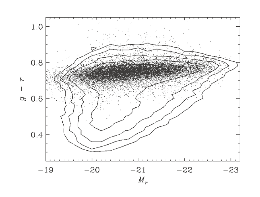
Figure 1.— Sample galaxies in the color-magnitude diagram. Points show the galaxies that meet the sample selection criteria described in §2, while contours show all galaxies at $0.04<z<0.08$. Galaxies in the sample are selected to be free of emission lines and to have light profiles characteristic of early type galaxies. No explicit color selection is applied, yet the resulting galaxy sample consists almost exclusively of red sequence galaxies. The remaining color outliers are not included in the stacked spectra. See §4.1 for details.

Throughout the rest of this paper, we will use velocity dispersion measurements that have been corrected to $1/8$ effective radius. Following Bernardi et al. (2003a) and Jørgensen et al. (1995), we use $\sigma=\sigma_{fib}(r_{fib}/\frac{1}{8}r_{\circ})^{0.04}$, where $r_{\circ}$ is the circular galaxy radius in arc seconds, computed as $r_{\circ}=R_{deV}\sqrt{(a/b)_{deV}}$, and $r_{fib}$ is the spectral fiber radius, 1.5^′′ for SDSS spectra. This allows us to provide consistent comparisons with past stellar population work, which typically uses central velocity dispersion measurements. In practice, velocity dispersion gradients are shallow, and this correction is small (of order $\sim 6$%). The $r$-band and $g$-band magnitudes used throughout this paper have been K-corrected to $z=0.0$ using the IDL code kcorrect v4.1.4 (Blanton et al. 2003) and converted to absolute magnitudes ($M_{r}$ and $M_{g}$) assuming a standard $\Lambda$CDM cosmology with $\Lambda=0.7$, $\Omega_{M}=0.3$ and $h=0.7$.

Spectra of the galaxies in our final sample were downloaded from the SDSS DR6 (Adelman-McCarthy 2007) version of the SDSS data archive server.

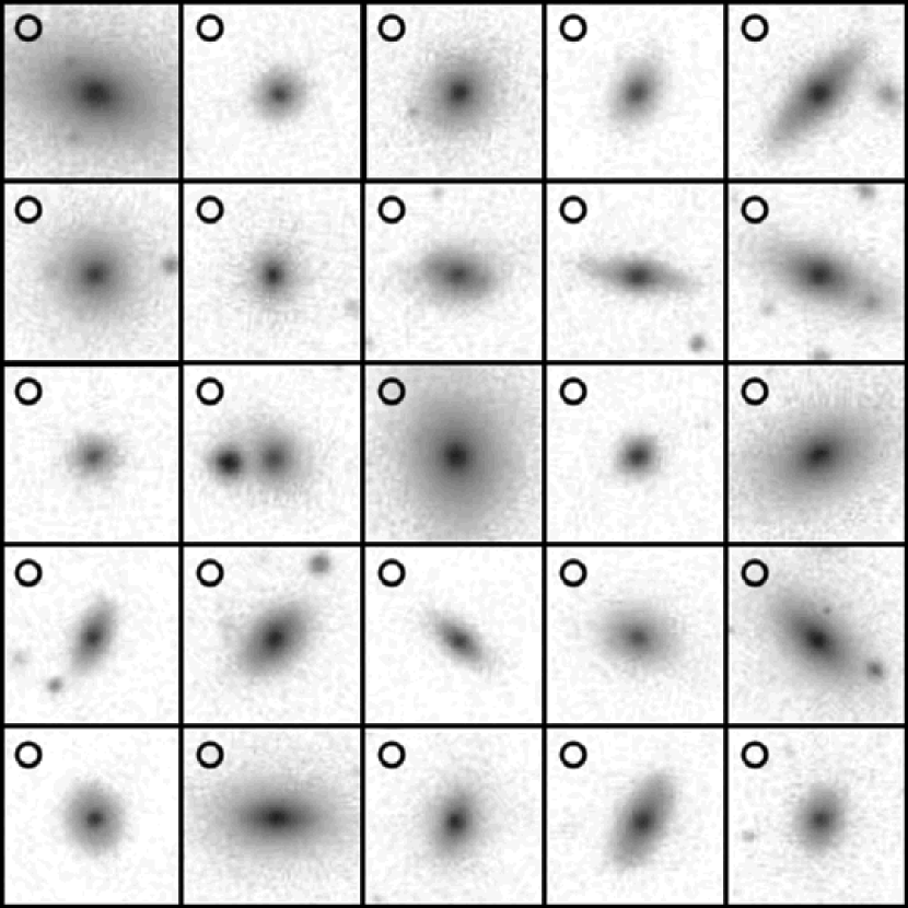
Figure 2.— Thumbnail images of a random selection of galaxies from the sample. Circles indicate the size of the 3^′′ SDSS spectral fibers. The sample is dominated by early type galaxies, but contains some bulge-dominated spirals as well at a range of orientations. Even where a disk is present, the spectral fiber predominantly samples light from the bulge.

2.2. Selection Criteria

To create a sample of passively evolving galaxies, we include only those galaxies with no emission from ionized gas. Specifically, we require that the measured equivalent widths of H$\alpha$ and [Oii]$\lambda$3727 emission be below a 2$\sigma$ detection threshold, as determined by Yan et al. (2006). In this sample, the typical 2$\sigma$ detection threshold corresponds to H$\alpha$ and [Oii] equivalent widths of $\sim 0.3$ Å and $\sim 1.7$ Å, respectively. This criterion excludes galaxies with significant ongoing star formation within the central portion of the galaxy covered by the spectral fiber, as well as active galactic nuclei (AGN) with optical emission lines (Yan et al. 2006).

Because the SDSS spectra only sample galaxy light with the 3^′′ spectral fiber radius, selecting quiescent galaxies in this way does not exclude disk galaxies with quiescent central bulge populations which harbor star formation in their outer regions. These galaxies are not truly quiescent galaxies, although they may have quiescent bulges. To limit contamination by these galaxies, we follow Bernardi et al. (2003a) in excluding galaxies with $R_{90}/R_{50}<2.5$ in the $i$-band (eliminating galaxies without centrally-concentrated light profiles) and for which the likelihood of a de Vaucouleurs light profile fit is less than 1.03 times the likelihood of an exponential fit. These further cuts reduce the sample size by $<10$%, leaving a total sample of 16,008 galaxies.

In summary, the galaxies in this study have been selected from the SDSS Main Galaxy Sample using the following criteria:

• Redshift range: $0.04<z<0.08$

• Apparent magnitude range: $15<r<18$

• No detected emission in H$\alpha$ and [Oii]$\lambda 3727$

• Concentrated light profiles: $R_{90}/R_{50}>2.5$ in the $i$-band

• Likelihood of a de Vaucouleurs light profile $\geq 1.03$ times larger than the likelihoood of an exponential light profile

Throughout the rest of this paper, we refer to the galaxies in our sample as quiescent or passive galaxies, with the understanding that this categorization refers to galaxies which are not actively forming stars.

In Figure 1, the galaxies used in this analysis are shown with respect to the color-magnitude distribution of all galaxies in this redshift range. The gray points show the galaxies included in the sample, while the contour lines show the underlying color-magnitude distribution of all galaxies with $0.04<z<0.08$ from the SDSS Main Galaxy spectroscopic sample. In choosing the sample presented here, no explicit color selection was applied, yet the resulting sample of galaxies populates a narrow red sequence relation between galaxy $M_{r}$ and color. Figure 2 shows thumbnail images for a randomly-selected set of galaxies from our final sample. The galaxies all have smooth morphologies. About 20% of the galaxies have significant disks, although all show evidence for prominant bulges. In the appendix, we show that the use of magnitudes and colors from de Vaucouleur fits to the galaxy light profiles (even in galaxies which have a disk component) has a negligible effect on our results.

Of our sample galaxies, 85% have bulge fractions above 0.8 while only 3% have bulge fractions below 0.5, making the sample galaxies highly bulge-dominated. Figure 2 shows that the sample contains a modest fraction of face-on and edge-on galaxy disks, however these do not dominate the light of the galaxies. Furthermore, the disk contribution to the measured spectrum will be substantially smaller than its contribution to the total galaxy light. The $3^{\prime\prime}$ SDSS spectral fibers (shown as circles in Figure 2) sample roughly 0.3–0.6 of the typical galaxy effective radius at these redshifts. In face-on disks, the SDSS $3^{\prime\prime}$ spectral fiber predominantly samples the galaxy bulge, while the spectra of inclined disks will contain a slightly increased light contribution from the galaxy disks. Edge-on disks in the sample must have negligible ongoing star formation in order to satisfy the stringent emission line cuts.

3. The Color-Magnitude Relation

The selection criteria defined above result in a sample of quiescent galaxies which populate the red sequence in the color-magnitude diagram. These galaxies show a clear color-magnitude relation (Figure 3, top panel), such that more luminous galaxies have redder colors. Data points are color-coded by bins in $\sigma$ as labelled in the lower figure panels. In the lower panels, the total galaxy sample is shown as a cloud of gray data points, with the total color-magnitude relation overplotted as the gray dotted line. In each panel, contours indicate the color-magnitude distribution of galaxies within a single bin in $\sigma$, as labeled. These $\sigma$ bins are used throughout this paper. The vertical dashed line in Figure 3 indicates the completeness limit of the SDSS Main Galaxy Sample in the redshift range used for this analysis. The solid line at $M_{r}=-19.7$ shows where we expect the sample is missing more than 50% of the galaxies at these magnitudes. Thus the lack of galaxies at fainter magnitudes is likely a selection effect rather than a genuine lack of galaxies at $M_{r}>-19.7$.

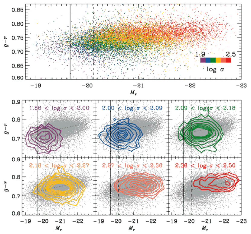
Figure 3.— Top panel: The color-magnitude relation for all galaxies in our sample. Data points are color-coded by $\sigma$, with purple (red) indicating the lowest (highest) $\sigma$ bin. The dashed vertical lines show the completeness limit of the sample, while the solid vertical lines show the magnitude at which the sample is missing 50% of the galaxies (i.e., where the sample becomes severely incomplete). Lower panels: The color–magnitude relation for galaxies at fixed $\sigma$. Gray points show the color-magnitude relation for the total galaxy sample, while over-plotted contours show the color-magnitude distribution of galaxies within a limited range in $\sigma$, as labeled. Contour lines indicate a number density of 5, 10, 20, 40, 60, 80, 100, and 120 galaxies per bin, where bins in $M_{r}$ and $g-r$ are defined by the tickmarks on the axes. The gray dotted line indicates the color-magnitude relation for the total sample. Galaxies with larger values of $\sigma$ tend to be brighter and redder than those at lower $\sigma$. However, galaxies at fixed $\sigma$ span a substantial range in both color and magnitude, so that different bins in $\sigma$ show a large amount of overlap in both color and magnitude. At fixed $\sigma$, there is no color-magnitude relation. Combining galaxies from all $\sigma$ bins results in an overall color-magnitude relation.

What is notable about the contours in Figure 3 is that they show no color-magnitude relation at fixed $\sigma$, in agreement with the work of Bernardi et al. (2005). In each panel, which illustrates a narrow range in $\sigma$, the contours in the color-magnitude diagram are horizontal. However, galaxies with larger $\sigma$ (red points) are generally more luminous and have redder colors than those with smaller $\sigma$ (blue and purple points), so that superposing the various $\sigma$ bins results in a net color-magnitude relation.

In contrast, the color-$\sigma$ relation is readily apparent at fixed $M_{r}$ (Figure 4, top). Here, colored data points indicate bins in luminosity, with dark green, light green, yellow, orange, pink, and purple data points corresponding to $-18.8>M_{r}>-20.0$, $-20.0>M_{r}>-20.4$, $-20.4>M_{r}>-20.8$, $-20.8>M_{r}>-21.2$, $-21.2>M_{r}>-21.6$, and $-21.6>M_{r}>-23$, respectively. A clear color-$\sigma$ relation is apparent at fixed $M_{r}$ (e.g., purple data points), with roughly the same slope at the total color-$\sigma$ relation. This color-$\sigma$ correlation is stronger and tighter than the color-magnitude relation shown in Figure 3.

Finally, the bottom panel of Figure 4 shows the $\sigma$-magnitude or Faber-Jackson relation, color-coded by galaxy $g-r$ color. Dark blue, medium blue, light blue, pale pink, medium pink, and dark pink data points represent $g-r<0.74$, $0.74<g-r<0.76$, $0.76<g-r<0.78$, $0.78<g-r<0.80$, $0.80<g-r<0.82$, and $0.82<g-r$, respectively. The $\sigma$-magnitude relation is tight for the most luminous galaxies, but shows considerable spread for faint galaxies. The spread is correlated with galaxy color, such that bluer galaxies tend to have lower $\sigma$ at fixed luminosity. This may indicate that fainter, bluer galaxies have a larger degree of rotational support, resulting in lower values of $\sigma$ for a given $M_{*}$.

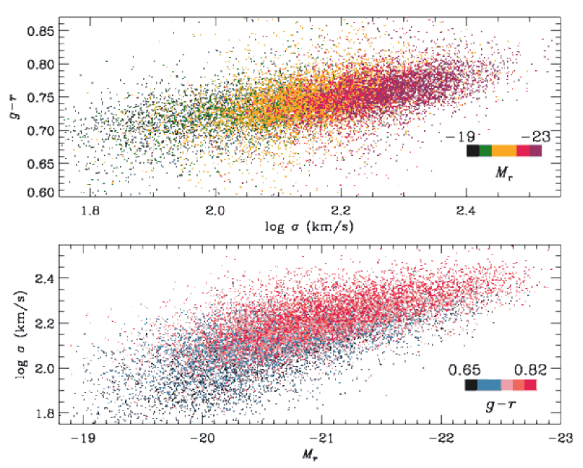
Figure 4.— Top panel: The color-$\sigma$ relation, with data points color-coded by galaxy luminosity. Dark green (purple) points show the faintest (brightest) luminosity bins. A color-$\sigma$ relation exists at fixed $M_{r}$ (e.g., purple data points alone) with roughly the same slope as the total color-$\sigma$ relation. The color-$\sigma$ trend is stronger and narrower than the color-magnitude relation in Figure 3. Bottom panel: The $\sigma$-magnitude relation, color-coded by galaxy $g-r$ color. Dark blue (dark pink) points show the bluest (reddest) galaxies. The $\sigma$-magnitude relation is broader for fainter galaxies. This is correlated with galaxy color, such that bluer galaxies tend to have lower $\sigma$ at fixed $M_{r}$. This may be due to a greater degree of rotational support in fainter and bluer early type galaxies, showing lower $\sigma$ for the same $M_{*}$.

It is clear that $\sigma$, luminosity, and color are all correlated in early type galaxies. Bernardi et al. (2005) argue that the fundamental relations are $\sigma$-color and $\sigma$-magnitude and that the color-magnitude relation results from a combination of these two correlations. The color-$\sigma$ relation (Figure 4, top) exists independent of galaxy luminosity (i.e., at fixed $M_{r}$). Likewise, the $\sigma$-magnitude relation (Figure 4, bottom) exists independent of galaxy color. However, the color-magnitude relation does not exist at fixed $\sigma$ (Figure 3), indicating that the $\sigma$ dependence of both color and magnitude is what leads to the observed color-magnitude relation.

From Figure 3, it is also clear that galaxies with very similar values of $\sigma$ show a substantial spread in $M_{r}$. The low–$\sigma$ bins suffer from incompleteness effects, but in the higher $\sigma$ bins (e.g., those with $\log\sigma\geq 2.18$), it is clear that galaxies with a range of only 0.09 dex in $\log\sigma$ span roughly 2 mag (0.8 dex) in $M_{r}$. Similarly, the substantial overlap of the $\sigma$ bins in the color-magnitude diagram means that galaxies at fixed $M_{r}$ have a range of $\sigma$.

These arguments illustrate that optical luminosity $L$ is not a good proxy for $\sigma$. This is expected from the fact that galaxies populate the FP and the Faber-Jackson relation is not an edge-on projection of the FP (Dressler et al. 1987). The two parameters are, however, often used interchangeably in the literature as measures of galaxy size or mass. We will see in §5.1 that using $L$ versus using $\sigma$ as the controlling variable in stellar population studies can lead to substantially different stellar population scaling relations, because stellar population properties vary systematically with $L$ at fixed $\sigma$.

4. Dissecting the Color-Magnitude Relation

Accurate stellar population parameters can only be derived from high $S/N$ spectra ($S/N\geq 100$ Å^-1; Cardiel et al. 1998). As individual SDSS galaxy spectra in our sample typically have $S/N\approx 20$ Å^-1, dozens or more spectra must be combined to achieve the necessary $S/N$. If galaxies are combined randomly, the average spectra would all look very similar. The challenge in this method is to identify useful ways of sorting the galaxies in advance, in order to do the best possible job of populating the full range of galaxy star formation histories, without averaging out all the interesting variations.

In this section, we define a three-dimensional parameter space of $\sigma$ (which is not sensitive to stellar population effects) along with $L$ and color (which are) and sort galaxies into bins in this space. We then stack the spectra of galaxies within each bin and measure absorption line strengths. In §5, we combine the observed line strengths with stellar population models to obtain the fundamental stellar population parameters of galaxies along and across the color-magnitude relation.

4.1. Binning by $\sigma$, $L$, and color

In §3, we divided our sample of quiescent galaxies into six bins based on $\sigma$. To study how stellar populations vary at fixed $\sigma$, we further divide those same $\sigma$ bins into three bins in color by three bins in $L$ for a total of 54 bins. Figure 5 illustrates this process for the $\log\sigma=2.18$–2.27 bin. Cuts in color and $L$ are defined with fixed width, such that each $L$ bin is 0.8 mag wide in $M_{r}$ and each color bin is 0.032 mag wide in $g-r$. The 3x3 grid of sub-bins is centered on the median $M_{r}$ and $g-r$ for all the galaxies in the given $\sigma$ bin. The median values of $\sigma$, $M_{r}$, and $g-r$ for each of the 54 bins are listed in Table 2, along with the total number of galaxies in each bin.

The central sub-bin in color–$L$ space contains more galaxies than the outer bins, but all bins are sufficiently well populated to produce high $S/N$ stacked spectra. Defining the color–$L$ grid in this way excludes color and $L$ outliers from each $\sigma$ bin, which ensures that the stacked spectra will not be biased by very deviant or misidentified objects.

In the lowest $\sigma$ bins, the magnitude limit of the sample presented here means that the fainter galaxies at that $\sigma$ are under-represented. Under the assumption that the missing faint galaxies at $z\sim 0.08$ are not substantially different from those at $z\sim 0.04$ which are included in the sample, the fainter bins are not strongly biased but are less populated than they ought to be. Comparisons between galaxies at different $L$ in the same $\sigma$ bin should therefore be robust to completeness effects. However, because these $\sigma$ bins are missing the faintest galaxies, the median $M_{r}$ used to locate the color–$L$ grid may be biased brighter than the underlying galaxy population at that $\sigma$.

4.2. Constructing the stacked spectra

In each of the 54 bins in $\sigma$–$L$–color space, we combine spectra of the galaxies in the bin in order to produce a very high $S/N$ average spectrum. Regions around the bright skylines at 5577Å, 6300Å, and 6363Å are masked in the individual galaxy spectra, which are then shifted to the restframe. The individual spectra are normalized so that all galaxies in the bin contribute equally to the averaged spectrum. The normalization uses the median flux in the 4100–5000Å range without modifying the continuum shape, as the flux-calibrated spectral shape affects the Lick index measurements. In practice, because the galaxies in a given bin have very similar colors, the shape of the continuum is nearly identical for all galaxies in the bin.

The stellar absorption features in higher $\sigma$ galaxies are effectively observed at lower resolution than those in lower $\sigma$ galaxies, due to the increased intrinsic Doppler smoothing of the lines from stellar motions within the galaxy. This intrinsic smoothing has non-negligible effects on the measured absorption line strengths. In order to compare all galaxies at the same effective resolution, we smooth lower–$\sigma$ galaxies up to match the highest-$\sigma$ galaxies in our sample, $\sigma\approx 300$ km s^-1. The algorithm we use to stack the galaxy spectra first averages the unsmoothed spectra of galaxies within narrow $\sigma$ sub-bins, with a routine that rejects very deviant pixels. The average clean sub-bin spectra are then smoothed to the maximum $\sigma$ of the sample ($\sim 300$ km s^-1) and coadded. The result is a stacked spectrum for each $\sigma$–$L$–color bin from which outlier pixels have been rejected and which has been smoothed to an effective resolution identical to all the other bins. The error spectrum is also computed from the individual SDSS galaxy error spectra by adding the individual pixel errors in quadrature to produce an error spectrum for each stacked spectrum.

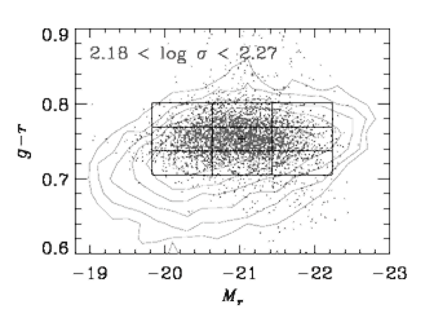
Figure 5.— Method used to bin galaxies by $L$ and color at fixed $\sigma$. The color-magnitude relation for the total quiescent galaxy sample in this typical $\sigma$ bin is indicated by the gray contours. Overplotted as gray points are all galaxies with $2.18<\log\sigma<2.27$. Within this $\sigma$ bin, there is no color-magnitude relation. The median point in $M_{r}$ and $g-r$ is shown as the black cross in the center. Galaxies in this $\sigma$ bin are divided into a 3x3 grid in color-magnitude space, with the grid centered on the median point and with fixed grid spacing of 0.8 mag in $M_{r}$ and 0.032 mag in $g-r$. Defining the grid in this way eliminates color and $L$ outliers which may bias the average properties of the bins. Galaxies in each of the six $\sigma$ bins are sorted in this way into nine sub-bins in color–$L$ space, and the galaxies in each sub-bin are stacked as described in §4.2 to produce high $S/N$ mean spectra for all 54 bins in $\sigma$–$L$–color space.

4.3. Lick Index absorption strengths

We measure the full set of Lick indices in each of the stacked spectra. These include the Balmer lines H$\beta$, H$\gamma_{F}$, and H$\delta_{F}$ (also broad definitions of H$\gamma_{A}$ and H$\delta_{A}$), and a set of Fe-dominated lines (Fe4383, Fe4531, Fe5015, Fe5270, Fe5335, Fe5406, Fe5709, and Fe5782), as well as numerous lines that are sensitive to abundances of elements other than Fe (Mg₁, Mg₂, Mg b, CN₁, CN₂, C₂4668, Ca4227, Ca4455, NaD, TiO₁, and TiO₂). The index definitions are taken from Worthey et al. (1994) and Worthey & Ottaviani (1997), and line strengths are measured using the Lick_EW code that is available online as part of the EZ_Ages code package (Graves & Schiavon 2008). The Lick_EW code also computes statistical errors for each Lick index based on the error spectra, using equations 33 and 37 of Cardiel et al. (1998). Because the Lick indices are defined as equivalent widths, they are insensitive to dust extinction effects.

All the stacked spectra have been smoothed to $\sigma=300$ km s^-1. Combined with the intrinsic resolution of the SDSS spectrograph, the spectra are at lower resolution than the Lick/IDS resolution at which the Lick indices are defined. A correction must be applied to the measured line strengths to bring them back onto the Lick index system. These corrections are included in the Lick_EW computation, based upon smooth single stellar population spectra, as given in Schiavon (2007) Table A2a. All of the spectra have been smoothed to the same $\sigma$ and corrected in the same way so that uncertainties in the velocity dispersion correction should not affect relative lines strength measurements. The corrected Lick index measurements and statistical errors for each of the 54 stacked spectra are given in Table 3. We do not attempt to match the zeropoints of the SDSS spectra to those of the Lick system as defined by Schiavon (2007). This should only introduce minor zero-point uncertainties because the Schiavon models are based on flux-calibrated spectra and the SDSS spectra are also flux calibrated (see Schiavon 2007, section 2.2.2).

4.4. Stellar population modelling

We compare the Lick index measurements for each of the stacked spectra to the stellar population models of Schiavon (2007) to derive fundamental stellar population parameters from the line strengths. The Schiavon (2007) models are single burst models which include the effect of variable abudance ratios by combining theoretical stellar isochrones (Girardi et al. 2000) with a library of empirical stellar spectra (Jones 1999) and individual line strength sensitivities to elemental abundance variations computed from theoretical stellar atmospheres (Korn et al. 2005). With these models, a set of Lick index measurements can be used to determine the mean luminosity-weighted stellar population age, iron abundance ([Fe/H]), and abundance ratios for the elements Mg, C, N, and Ca ([Mg/Fe], [C/Fe], [N/Fe], and [Ca/Fe]) using the algorithm described in Graves & Schiavon (2008) and implemented in the publicly available code EZ_Ages. Briefly, the Graves & Schiavon (2008) method determines a fiducial mean age and [Fe/H] from a combination of Balmer and Fe-dominated indices, then uses other indices which are sensitive to Mg, C, N, and Ca to adjust the element abundance ratios until the model index predictions match the ensemble of Lick index data. The basic modelling process has not changed since the original analysis of red sequence galaxies with LINER-like emission in Graves et al. (2007); subsequent minor updates to the EZ_Ages code have improved the robustness of the code at runtime and produce results that match those of Graves et al. (2007) within the quoted errors. EZ_Ages estimates stastical errors for each of the stellar population parameters, based on the measurements errors in the Lick indices. The errors in these various parameters are not independent; an analysis of the correlated errors is presented in Figure 3 of Graves & Schiavon (2008). The reader is referred to that article for additional details on the age and abundance fitting process.

Graves & Schiavon (2008) have shown that this fitting method is robust to the choice of Lick indices used in the analysis. Here we use the “standard set” of Lick indices from Graves & Schiavon (2008)—H$\beta$, $\langle$Fe$\rangle$ (which is an average of the Fe5270 and Fe5335 indices), Mg b, C₂4668, CN₁, and Ca4227—with the EZ_Ages code to fit a mean luminosity-weighted age, [Fe/H], [Mg/Fe], [C/Fe], [N/Fe], and [Ca/Fe] for each of the 54 average galaxy spectra. We can thus track each of these stellar population parameters as a function of $\sigma$, $L$, and color for the galaxies in our sample.

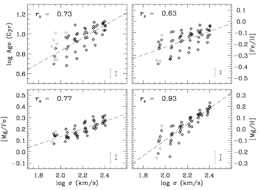
Figure 6.— Mean stellar population parameters for each of the 54 stacked galaxy spectra, shown as a function of median $\sigma$ for the galaxies in each bin. The error bars in the lower right corner of each panel show the median statistical error in the derived population parameters, based on the uncertainties in the Lick index measurements. The data have been separated into those with small statistical errors (black) and those with larger statistical errors (gray), as indicated by the corresponding error bars. “Large” statistical errors are defined as those more than two standard deviations larger than the median error. Mean luminosity-weighted stellar age, [Fe/H], [Mg/H], and [Mg/Fe] all increase with increasing $\sigma$. Dashed lines show linear least squares fits of the stellar population properties onto $\log\sigma$, computed using the black data points only. The Spearman rank correlation coeffecients ($r_{s}$) of the correlations are specified in each panel. The scatter in mean age and [Fe/H] is significantly larger than that expected due to measurement errors, implying genuine variation in these population parameters at fixed $\sigma$. The spread in age is small for the highest–$\sigma$ galaxies, all of which show old ages, while the lowest–$\sigma$ galaxies cover a substantial factor in mean age. There is only modest scatter in either [Mg/Fe] or [Mg/H] at fixed $\sigma$. The correlation bewteen $\sigma$ and [Mg/H] is particulary strong, as indicated by the very high value of $r_{s}$.

In this analysis, we focus on the stellar population age, [Fe/H], [Mg/H], and [Mg/Fe], leaving the analysis of other abundance ratios for future work. The results of the stellar population analysis for the stacked spectra are presented in Table 3. Of the $\alpha$-elements, Mg is the only one that is relatively straightfoward to measure in optical galaxy spectra. For the purposes of this type of stellar population work, it is typically assumed that all $\alpha$-elements scale together and thus that [Mg/Fe] is equivalent to [$\alpha$/Fe]. There is some observational evidence that $\alpha$ elements may not always vary in lock-step (e.g., Fulbright et al. 2007; Humphrey & Buote 2006) but, lacking an alternative, we will use [Mg/Fe] as an estimate of the total [$\alpha$/Fe]. The Schiavon (2007) models are computed at fixed [Fe/H] rather than at fixed total metallicity ([Z/H]), so that enhancements in individual elements also change the total metallicity of the galaxy.

It is important to keep in mind that the stellar population parameters based on modelling absorption line indices give ages and abundances averaged over the ensemble of stars in the galaxy. The contribution of each star to the average age or abundance measurement is proportional to the light contributed at the wavelength of the absorption feature in question, and also to the equivalent width of the particular absorption feature of that star. When comparing ages of galaxies, a younger mean luminosity-weighted age in one galaxy compared to another does not necessarily mean that all of the stars in the galaxy are younger: a galaxy may contain a fraction of young stars that skew the average age to lower values. The luminosity-weighted ages presented here are also averaged over the ensemble of galaxies in the bin and should thus be treated as a statistical description of galaxies in that bin rather than as “true” ages for all of the stars in an individual galaxy.

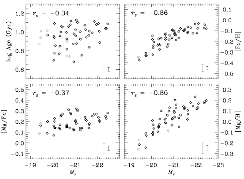
Figure 7.— Mean stellar population parameters as a function of galaxy $L$. The results of the stellar population analysis are plotted against the median $M_{r}$ for the galaxies in each bin. Statistical errors in the derived population parameters are shown in the lower right corner of each panel. The data have been separated into those with small statistical errors (black) and those with larger statistical errors (gray), as indicated by the corresponding error bars. The Spearman rank correlation coefficient ($r_{s}$) is given for each relation. The strong increases in mean age and [Mg/Fe] visible in Figure 6 when plotted against $\sigma$ are considerably washed out when plotted against $M_{r}$, while the trend between [Fe/H] and $M_{r}$ is much tighter than the $\sigma$–[Fe/H] relation. The [Mg/H]–$M_{r}$ is still strong, although $r_{s}$ indicates it is slightly weaker than the $\sigma$–[Mg/H] correlation.

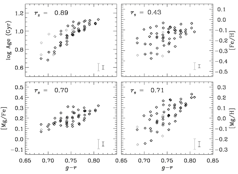
Figure 8.— Mean stellar population parameters as a function of galaxy color. The results of the stellar population analysis are plotted against the median $g-r$ color for the galaxies in each bin. Statistical errors in the derived population parameters are shown in the lower right corner of each panel. The data have been separated into those with small statistical errors (black) and those with larger statistical errors (gray), as indicated by the corresponding error bars. The Spearman rank correlation coefficienct ($r_{s}$) is given for each relation. Here, mean age increases with color, similar to the $\sigma$–age trend observed in Figure 6 although with somewhat smaller scatter in log age at fixed $g-r$ than was seen at fixed $\sigma$. However, [Fe/H] shows only a very weak trend with color, while [Mg/Fe] and [Mg/H] increase significantly in redder galaxies. Neither the [Mg/Fe]–color nor [Mg/H]–color trends are as strong as the those with $\sigma$, as indicated by $r_{s}$.

5. Stellar Populations on the Red Sequence

5.1. Age, [Fe/H], [Mg/H], and [Mg/Fe] as Functions of $\sigma$, $L$, and Color

Figure 6 shows the age, [Fe/H], [Mg/H], and [Mg/Fe] results of the stellar population analysis as a function of galaxy $\sigma$. The stellar population parameters derived from the stacked spectra are plotted against the median value of $\sigma$ for the ensemble of galaxies in each of the 54 bins. The median statistical errors in the derived population parameters are shown in the lower right corner of each panel. The Spearman rank correlation coefficient ($r_{s}$) is shown for each pair of parameters, indicating the strength of the correlation. Age, [Fe/H], [Mg/H], and [Mg/Fe] all show correlations with $\sigma$, such that higher–$\sigma$ galaxies have older mean ages, higher iron abundances, higher magnesium abundances, and higher levels of Mg-enhancement, which strongly suggests that higher–$\sigma$ galaxies also have higher total metallicities. These results are in agreement with numerous previous authors (e.g., Bernardi et al. 2003b; Thomas et al. 2005; Nelan et al. 2005; Smith et al. 2007a; see summary in Table 8 of Graves et al. 2007), although these trends are not universally observed in all early type galaxy samples (e.g., Kelson et al. 2006; Trager et al. 2008).

The [Mg/H]-$\sigma$ and [Mg/Fe]-$\sigma$ relations are particularly tight compared to the typical measurement errors. This implies that at fixed $\sigma$ [Mg/H] and [Mg/Fe] vary only weakly with the other two global parameters studied here ($L$ and color). At high $\sigma$, [Mg/H] shows almost no variation at fixed $\sigma$. A linear least-squares fit of [Mg/Fe] onto $\sigma$ gives a slope of 0.34, which is consistent with previous results.

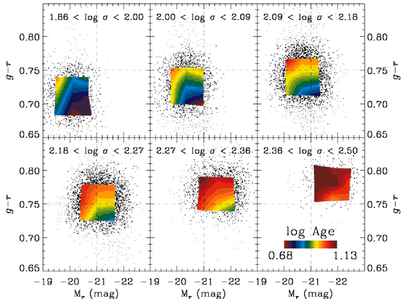
Figure 9.— Mean luminosity-weighted age as a function of $\sigma$, $L$, and color. Each panel shows the color-magnitude diagram for a slice in $\sigma$, corresponding to the six $\sigma$ bins in Figure 3. Black points represent galaxies that fall within 1.2 mag of the median $M_{r}$ and within 0.048 mag of the median $g-r$ for the $\sigma$ bin. Gray points show galaxies that fall outside these boundaries and which are excluded from the stacked spectra, as described in §4.1. Overplotted are contours of mean luminosity-weighted galaxy age, derived from the stellar population modelling in §4.4. The dashed lines are reference lines to guide the eye when comparing between $\sigma$ bins. Stellar population age increases with increasing $\sigma$, but shows substantial scatter within a fixed $\sigma$ slice. There is more age variation amongst low–$\sigma$ galaxies than in high–$\sigma$ galaxies. At fixed $\sigma$, lines of constant age run roughly diagonally across the color-magnitude diagram, with younger galaxies having bluer colors and brighter luminosities, while older galaxies have redder colors and fainter luminosities. When the various $\sigma$ slices are stacked together into the observed red sequence, the decrease in age with $L$ at fixed $\sigma$ counter-acts the overall increase of age with $\sigma$, erasing the age trend when $L$ is used to parameterize galaxies instead of $\sigma$ (as in Figure 7). See §5.2 for details.

Unlike [Mg/H] and [Mg/Fe], both age and [Fe/H] show scatter at fixed $\sigma$ that is large compared to the statistical error bars. For [Fe/H], the scatter is roughly the same at all $\sigma$, whereas the spread in mean ages at fixed $\sigma$ appears to be larger for lower–$\sigma$ galaxies. It is noteworthy that some low–$\sigma$ galaxies have mean ages nearly as old as some of the highest-$\sigma$ galaxy bins. Thus any model for galaxy formation that predicts a correlation between galaxy $\sigma$ and galaxy age must also be able to accommodate low–$\sigma$ galaxies with old ages.

Because $\sigma$ correlates with both $L$ and color (see §3), one might expect to see similar correlations between stellar population properties and $L$ or color as were seen for $\sigma$. Figure 7 shows the derived stellar population parameters as functions of $L$, while Figure 8 shows the same as functions of galaxy color. Interestingly, when the stellar population properties are plotted against $L$ instead of $\sigma$, the correlations with age and [Mg/Fe] are nearly erased, while the correlation with [Fe/H] is much tighter. Conversely, when they are plotted against color, the correlation with mean stellar age is slightly tighter than with $\sigma$, while the [Fe/H] and [Mg/Fe] correlations are weaker than with $\sigma$. Of the four stellar population parameters, [Mg/H] alone shows relatively strong correlations with all three global parameters, although it is most strongly correlated with $\sigma$.

Figures 6–8 show that, although $\sigma$, $L$, and color are all correlated with one another, the various stellar population parameters show significantly different behavior with each of the global parameters. Residuals from the $\sigma$–stellar population relations must correlate with $L$ and color in such a way as to erase some trends and strengthen others when $L$ or color are used instead of $\sigma$. This correlation of residuals immediately suggests that quiescent galaxies populate a multi-dimensional stellar population parameter space. To explore these effects in detail, we must investigate the dependence of stellar age, [Fe/H], [Mg/H], and [Mg/Fe] on all three global parameters simultaneously.

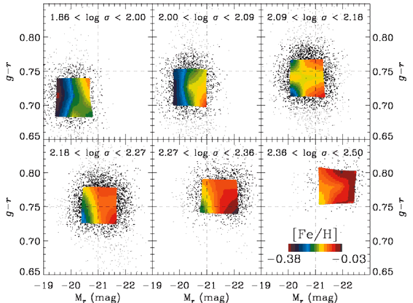
Figure 10.— [Fe/H] as a function of $\sigma$, $L$, and color. As in Figure 9, panels show the color-magnitude diagram for slices of fixed $\sigma$. Black points show galaxies included in the stacked spectra, while gray points show color and $M_{r}$ outliers that have been excluded from this analysis. Overplotted are contours of [Fe/H] derived from the stellar population modelling of §4.4. [Fe/H] increases with increasing $\sigma$. Lines of constant [Fe/H] run approximately vertically in color-magnitude space at fixed $\sigma$, with the most luminous galaxies being the most Fe-rich. When the various $\sigma$ slices are stacked together into the observed color-magnitude relation, the increase in [Fe/H] with $L$ at fixed $\sigma$ reinforces the increase in [Fe/H] with $\sigma$, causing the $L$–[Fe/H] relation to be tighter and steeper than the $\sigma$–[Fe/H] relation. Comparisons with Figure 9 show that, at fixed $\sigma$, age and [Fe/H] are roughly anti-correlated, helping to preserve the tightness of the total color–$\sigma$ relation.

5.2. Mapping Stellar Populations Across the Red Sequence

Figure 9 shows contours of stellar population age as a function of $\sigma$, $L$, and color. The six panels contain data for our six standard $\sigma$ slices corresponding to the panels in Figure 3. Black and gray data points in each panel show the color-magnitude relation at that $\sigma$, with gray points indicating galaxies in the $\sigma$ range which were excluded from the stacked spectra.

Plotted over the color-magnitude relations in each bin are color contours representing the mean luminosity-weighted ages derived from the stacked spectra. The age contours were constructed as follows: age values from the stacked spectra in each $\sigma$ range were plotted at the median values of $M_{r}$ and $g-r$ for each bin, forming a 3x3 grid of age values in color-magnitude space. Values of age were linearly interpolated (in log age) between the nine grid points to produce age contours across the color-magnitude relation. The color bar in the lower right panel indicates the scaling of the age contours, with the lowest and highest values indicated. The dashed lines at $M_{r}=-21$ and $g-r=0.75$ are the same in all panels and exist merely to guide the eye. As $\sigma$ increases, galaxies become systematically both brighter and redder with respect to the dashed lines.

The age contours in Figure 9 illustrate the same trends that were visible in Figure 6. As $\sigma$ increases from low (upper left panel) to high values (lower right panel), the average age indicated by the contours increases. However, in each slice in $\sigma$, a range of ages exists. The spread in ages at fixed $\sigma$ is large in the low–$\sigma$ bins and becomes increasingly smaller toward the highest–$\sigma$ bins.

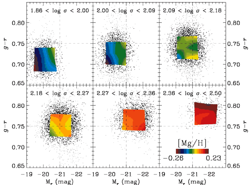
Figure 11.— [Mg/H] as a function of $\sigma$, $L$, and color. Panels show the color-magnitude diagram for slices of fixed $\sigma$. Black points shows galaxies included in the stacked spectra, while gray points show color and $M_{r}$ outliers that have been excluded from this analysis. Overplotted are contours of [Mg/H] derived from the stellar population modelling of §4.4. Mg is used to trace $\alpha$-elements, thus contours of [Mg/H] here are a proxy for contours of [$\alpha$/H]. [Mg/H] increases with increasing $\sigma$, showing the least variation at fixed $\sigma$ of any of the stellar population parameters. In the lower–$\sigma$ bins, [Mg/H] behaves similarly to [Fe/H], with lines of constant [Mg/H] running nearly vertically in color–magnitude space.

The contours also illustrate the behavior of stellar population age at fixed $\sigma$ across the color-magnitude relation. Lines of constant age thus run roughly diagonally in color-magnitude space at fixed $\sigma$, with young ages in the lower right corner (bright and blue) and old ages in the upper left corner (faint and red). This trend is approximately repeated in each $\sigma$ slice, although at high $\sigma$ the dynamic range is less. The variation at fixed $\sigma$ cannot be explained by errors in $\sigma$ that result in galaxies being assigned to the wrong stacked spectrum because this would result in the opposite effect: galaxy contamination from higher–$\sigma$ bins would tend to make the more luminous galaxies appear older, not younger.

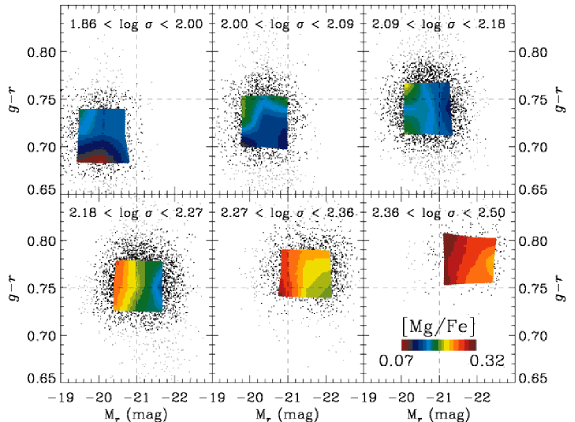
Figure 12.— [Mg/Fe] as a function of $\sigma$, $L$, and color. Panels show the color-magnitude diagram for slices of fixed $\sigma$. Black points shows galaxies included in the stacked spectra, while gray points show color and $M_{r}$ outliers that have been excluded from this analysis. Overplotted are contours of [Mg/Fe] derived from the stellar population modelling of §4.4. Mg is used to trace $\alpha$-elements, thus contours of [Mg/Fe] here are a proxy for contours of [$\alpha$/Fe]. [Mg/Fe] increases with increasing $\sigma$. There is limited variation in [Mg/Fe] at fixed $\sigma$. A comparisons with Figure 9 shows that [Mg/Fe] varies similarly to age, such that fainter galaxies at fixed $\sigma$ are older and have higher [Mg/Fe]. This variation runs in the opposite sense of variation in [Fe/H] at fixed $\sigma$, which increases with increasing luminosity. When the various $\sigma$ slices are stacked together in the observed red sequence, the decrease of [Mg/Fe] with increasing $L$ at fixed $\sigma$ counter-acts the trend of increasing [Mg/Fe] with increasing $\sigma$, thus the $\sigma$–[Mg/Fe] relation is substantially weakened when $L$ is used to parameterize galaxies instead of $\sigma$

Figure 10 shows the same slices through the color-magnitude relation, this time with color contours indicating [Fe/H]. Again, the trends of Figure 6 are visible: [Fe/H] increases with $\sigma$ from the lowest–$\sigma$ bins to the highest, and a range in [Fe/H] exists within each slice in $\sigma$. However, the variation in [Fe/H] at fixed $\sigma$ is markedly different from the age variation seen in Figure 9. Lines of constant [Fe/H] run nearly vertically in the color-magnitude diagram for fixed $\sigma$, such that more luminous galaxies have higher [Fe/H].

The contours of [Mg/H] shown in Figure 11 are similar to those in [Fe/H] for the same $\sigma$ slices through the color-magnitude relation. In addition to the total increase in [Mg/H] with $\sigma$, the brightest galaxies at fixed $\sigma$ have the highest values of [Mg/H]. However, [Mg/H] shows less variation at fixed $\sigma$ than does [Fe/H], particularly in the high–$\sigma$ bins. This is as expected from Figure 6. Although the spread in [Mg/H] at fixed $\sigma$ seen here and in Figure 6 is small, Figure 11 strongly suggests that these variations are in fact real because they are consistent across the $\sigma$ bins.

Finally, Figure 12 shows $\sigma$ slices overlaid with contours of constant [Mg/Fe], directly comparing the differences in Fe and Mg enrichment. Again, [Mg/Fe] increases with increasing $\sigma$, as expected from Figure 6. Like [Mg/H], the variation at fixed $\sigma$ is mild and therefore somewhat more difficult to categorize than the variation in age and [Fe/H], but broadly [Mg/Fe] behaves similarly to age, showing larger enhancements in fainter galaxies at fixed $\sigma$. Because Mg is produced by supernovae Type II (SNe II) on short timescales while Fe is produced by supernovae Type Ia (SNe Ia) on longer timescales, the observed overabundance of Mg relative to the solar abundance pattern is typically interpreted to indicate a short timescale for star formation, leaving the stellar population of the galaxy enhanced in SN II products but not in SN Ia products.

These maps of age, [Fe/H], [Mg/H], and [Mg/Fe] across the color-magnitude relation confirm that quiescent galaxies form a multi-parameter family in stellar population properties. Age, [Fe/H], [Mg/H], and [Mg/Fe] all increase with $\sigma$, but show variations at fixed $\sigma$ depending on their $L$. Of the four stellar population parameters presented in Figures 9–12, only age shows a strong dependence on color as well as $L$. Variations in age and [Mg/Fe] with $L$ at fixed $\sigma$ are similar (both increase toward fainter galaxies) and are opposite to the variations in [Fe/H] and [Mg/H] (both of which increase toward brighter galaxies). This suggests that the oldest galaxies in the universe formed their stars over short timescales, while younger quiescent galaxies experienced more extended star formation.

Using these stellar population maps, the differing trends with $\sigma$ and with $L$ illustrated in Figures 6 and 7 can be understood by superposing the various $\sigma$ slices of the color-magnitude relation. Although we have seen that age and [Fe/H] both increase with $\sigma$, Figures 9 and 10 show that age and [Fe/H] exhibit opposite behavior from one another at fixed $\sigma$, namely that age decreases and [Fe/H] increases for brighter galaxies at fixed $\sigma$. Because of this difference, superposing the various $\sigma$ slices to form the total color-magnitude relation acts to reinforce the $\sigma$–[Fe/H] relation into an even tighter $L$–[Fe/H] relation. At the same time, the age trends at fixed $\sigma$ counteract the $\sigma$–age relation, resulting in almost no $L$–age relation. The explains why stellar population studies as a function of $L$ or $M_{*}$ find weak or non-existant $L$–age relations (e.g., Kuntschner & Davies 1998; Terlevich & Forbes 2002; Gallazzi et al. 2005), while stellar population studies as a function of $\sigma$ turn up significant $\sigma$–age correlations (e.g., Bernardi et al. 2003b; Thomas et al. 2005; Nelan et al. 2005; Smith et al. 2007a; Graves et al. 2007).

In this scenario, although the $L$–[Fe/H] correlation is stronger than the $\sigma$–[Fe/H] correlation, we interpret the $\sigma$–[Fe/H] trend as the primary relation, with the increased tightness of the $L$–[Fe/H] relation being caused by correlated residuals from the $\sigma$–$L$ and $\sigma$–[Fe/H] relations. In the next section, we use principal components analysis to show that the family of stellar populations in quiescent galaxies is nearly two-dimensional, with the first dimension parameterized by $\sigma$ and the second dimension parameterized by correlated residuals from the various $\sigma$–$L$, $\sigma$–color, and $\sigma$–stellar population trends.

5.3. Principal Components Analysis and Stellar Population Residuals

To quantitatively explore the multi-dimensional space of global and stellar population parameters illustrated in the previous section, we have performed a principal components analysis (PCA; see, e.g., Faber 1973; Trager et al. 2000) in the seven dimensional space parameterized by $\sigma$, $L$, color, age, [Fe/H], [Mg/H], and [Mg/Fe]. All parameters are “standardized” to have a mean of zero and a variance of one before performing the PCA. The results are shown in Table 1. Although the parameter space is nominally seven dimensional, there are only six principal components (PCs) because [Mg/H] $\equiv$ [Mg/Fe] $+$ [Fe/H]. The first two PCs account for 91% of the variance in the population, indicating that the quiescent galaxy population can be well-described by a two-dimensional hyperplane.

The first PC (PC1) accounts for a full 70% of the observed variation and is comprised of positive contributions from all of the input parameters. This illustrates quantitatively that all the parameters presented here are correlated with one another. We saw in §3 that the color-magnitude relation is the result of fundamental $\sigma$-color and $\sigma$-magnitude relations. It therefore seems reasonable to treat $\sigma$ as the primary global parameter behind PC1.

Table 1Principal Component Analysis

Parameter	PC1	PC2	PC3	PC4	PC5	PC6
log $\sigma$	$0.43$	$0.03$	$0.31$	$0.37$	$-0.53$	$0.55$
log $L$	$0.37$	$-0.40$	$0.04$	$0.59$	$0.58$	$-0.14$
$g-r$	$0.40$	$0.23$	$-0.62$	$-0.25$	$0.32$	$0.50$
log Age	$0.32$	$0.53$	$-0.33$	$0.32$	$-0.27$	$-0.57$
[Fe/H]	$0.32$	$-0.55$	$-0.22$	$-0.29$	$-0.33$	$-0.21$
[Mg/H]	$0.43$	$-0.21$	$0.14$	$-0.40$	$-0.08$	$-0.21$
[Mg/Fe]	$0.36$	$0.39$	$0.59$	$-0.34$	$0.31$	$-0.11$
Eigenvalue	$4.88$	$1.49$	$0.35$	$0.18$	$0.07$	$0.03$
Percentage of variance	69.7	21.3	5.0	2.6	1.0	0.4
Cumulative percentage	69.7	91.0	96.0	98.6	99.6	100.0

Note. — Parameters are “standardized” to have a mean of zero and a variance of one before performing PCA. Although seven parameters are reported here, there are only six principal components because [Mg/H] $\equiv$ [Fe/H] $+$ [Mg/Fe].

The second PC (PC2) encompasses another 21% of the variance and includes significant contributions from all parameters except for $\sigma$. PC2 therefore represents the correlated residuals from the mean relations between $\sigma$ and the other parameters. The contributions of $g-r$, age, and [Mg/Fe] to PC2 are positive while those of $L$, [Fe/H], and [Mg/H] are negative. This indicates that at fixed $\sigma$, $g-r$, age, and [Mg/Fe] are correlated with one another and are anti-correlated with $L$, [Fe/H], and [Mg/H]. Of the global parameters, $L$ contributes the most to PC2.

5.4. Stellar Population Residuals from $\sigma$ Relations

Residuals in the four stellar population parameters ($\Delta\log$ age, $\Delta$[Fe/H], $\Delta$[Mg/H], and $\Delta$[Mg/Fe]) are defined as the difference between the observed values and the mean relations with $\sigma$, as indicated by the dashed lines in Figure 6. The correlated stellar population residuals associated with PC2 are shown in Figure 13. In each panel, high and low $S/N$ data are indicated by filled and open circles, respectively. The error ellipses in the lower left corner of each panel indicate the stastical errors from the stellar population modelling process, with solid black (dashed gray) lines showing the median statistical errors for high (low) $S/N$ data. Measurement errors in the index absorption line strengths produce correlated errors in the derived stellar population parameters. These are determined from Monte Carlo simulations in Graves & Schiavon (2008) and are indicated by the error ellipse orientation. In all panels, residuals are color-coded by luminosity residuals; the green circles represent the central bin in $L$ at fixed $\sigma$ (centered on the median $L$ for that $\sigma$, as in Figure 5) while blue and red circles indicate brighter ($\Delta L\approx-0.8$ mag in $r$) and fainter ($\Delta L\approx+0.8$ mag in $r$) luminosity bins.

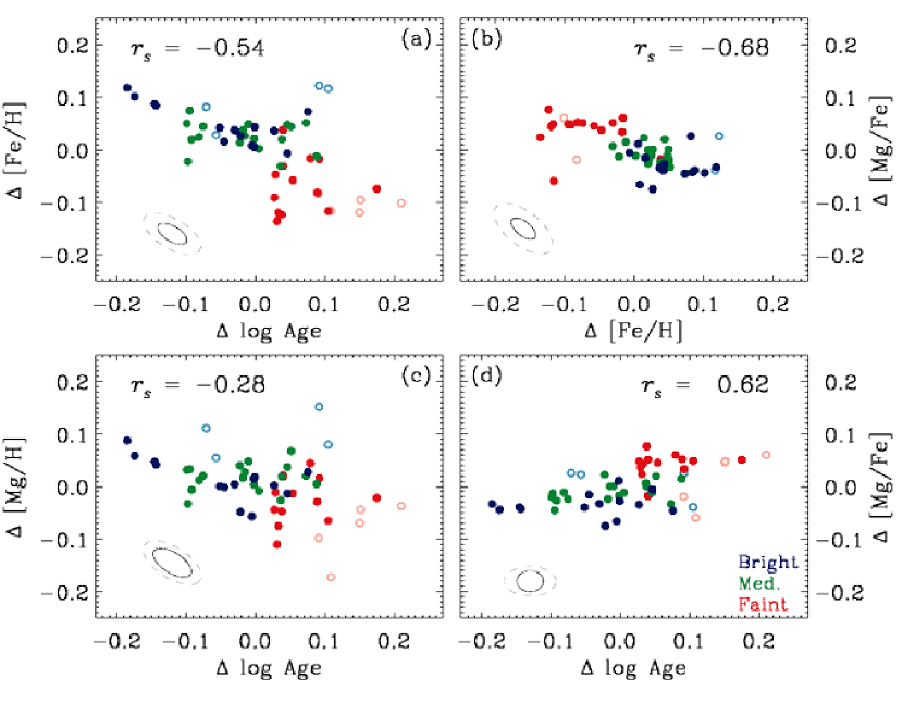
Figure 13.— Correlated residuals in stellar population parameters at fixed $\sigma$. Residuals $\Delta\log$ Age, $\Delta$[Fe/H], $\Delta$[Mg/H], and $\Delta$[Mg/Fe] were computed by subtracting off the trends with $\sigma$ (dashed lines in Figure 6) from the observed values. Data are color-coded by luminosity bin ($\Delta L$) as indicated. Filled (open) circles show high (low) $S/N$ data, while solid (dashed) error ellipses show the corresponding correlated errors from stellar population modelling. The Spearman rank correlation coefficient ($r_{s}$) is indicated for each pair of residuals. Residuals from the mean relations with $\sigma$ are related such that residuals in age and [Mg/Fe] are correlated with one another and are anti-correlated with residuals in [Fe/H] and [Mg/H]. These correlated residuals are also correlated with $\Delta L$, such that the brighter galaxies (blue points) at a given $\sigma$ have lower ages, lower [Mg/Fe], higher [Fe/H], and higher [Mg/H] than their fainter counterparts (red points). Although the residuals are in many cases correlated in the same direction as the correlated errors from stellar population modelling, the relation between the stellar population residuals and $\Delta L$ could not be produced by stellar population modelling errors and indicates that the residual correlations are real.

Panel (a) shows an anti-correlation between $\Delta\log$ age and $\Delta$[Fe/H], such that older galaxies are typically Fe-poor compared to younger galaxies at the same $\sigma$. This anti-correlation at fixed $\sigma$ has been reported by numerous previous authors (e.g., Worthey et al. 1995; Colless et al. 1999; Jørgensen 1999; Trager et al. 2000) and was quantified by Trager et al. (2000) as the “metallicity hyperplane”. The anti-correlation conspires to keep the color–$\sigma$ relation tight (c.f., Figure 4). In contrast to the observed age–[Fe/H] anti-correlation at fixed $\sigma$, we saw in Figure 7 that at fixed $L$, there is significant scatter in age but almost no scatter in [Fe/H] (although see Poggianti et al. 2001). This implies that age differences will produce color variations at fixed $L$ which cannot be offset by correlated variations in [Fe/H]. Thus, the color-magnitude relation should show more color variation at fixed $L$ than is observed in the color-$\sigma$ relation at fixed $\sigma$, consistent with Figures 3 and 4. Furthermore, the observed color spread in the color-magnitude relation should correlate with age, such that bluer galaxies are younger than redder galaxies at fixed $L$. This is consistent with Figure 9 and also with the results of Cool et al. (2006).

In addition to the age–[Fe/H] anti-correlation evident in Figure 13a, a similar anti-correlation is present between age and [Mg/H] (Figure 13c), although it is significantly weaker. A further anti-correlation is observed between [Fe/H] and [Mg/Fe] (Figure 13b), such that Fe-poor galaxies are more Mg-enhanced than their comparitively Fe-rich counterparts at fixed $\sigma$. Finally, Figure 13d shows a positive correlation between age and [Mg/Fe], such that older galaxies are more Mg-enhanced with respect to the solar abundance pattern than their younger counterparts at fixed $\sigma$.

In panels a–c, the slopes of the observed anti-correlations are similar to those expected from correlated errors in stellar population modelling, as indicated by the error ellipses. However, the observed anti-correlations cannot be due to correlated statistical errors for several reasons. Firstly, the typical statistical errors are too small to produce the observed spread in stellar population properties. More conclusively, if the observed anti-correlations were due to measurement errors, they would not be systematically correlated with $\Delta L$. The observed $L$–dependence of stellar population properties at fixed $\sigma$ argues strongly that the anti-correlation is real. In appendix B, we verify that the observed anti-correlations are not due to systematic effects in the stellar population modelling process caused by using single burst models to fit integrated galaxy spectra, which are almost certainly not single burst populations.

It is evident from Figure 13 that, not only are the various stellar population residuals correlated with one another, they are also strongly correlated with $\Delta L$, as quantified by the PCA analysis in the previous section. Collecting all parameters together, the residual trends can be summarized as follows: at fixed $\sigma$, galaxies fainter than the median are older, Fe-poor, somewhat Mg-poor, and more Mg-enhanced than typical galaxies at that $\sigma$, while galaxies brighter than the median are younger, Fe-rich, somewhat Mg-rich, and less Mg-enhanced.

6. Discussion

We have shown that (1) stellar population age, [Fe/H], [Mg/H], and [Mg/Fe] all increase with increasing galaxy $\sigma$ (Figure 6), and (2) that the star formation histories of galaxies vary systematically at fixed $\sigma$ such that fainter galaxies are older, Fe-poor, and Mg-enhanced compared to their bright counterparts at the same $\sigma$ (Figure 13). The first of these results is in agreement with a substantial number of earlier works (e.g, Bernardi et al. 2003b; Thomas et al. 2005; Nelan et al. 2005; Smith et al. 2007a; Graves et al. 2007). In particular, the increase in age with $\sigma$ is consistent with “archeological downsizing” (Thomas et al. 2005), in which massive galaxies form their stars predominantly at early times, while lower mass galaxies show evidence of younger stellar populations.

The anti-correlation of age and [Fe/H] at fixed $\sigma$ shown in this analysis is not a new result and is in agreement with the metallicity hyperplane of Trager et al. (2000) and with the recent work of Smith et al. (2007b) for individual galaxies. However, an important new result of this work is that this anti-correlation is correlated with galaxy luminosity, such that the more luminous galaxies at fixed $\sigma$ are the younger, Fe-rich galaxies while the fainter galaxies are older and more Fe-poor. This confirms that the observed anti-correlation of age and [Fe/H] must be genuine, rather than an effect of correlated stellar population modelling errors.

The co-variation of age, [Fe/H], and [Mg/Fe] we observe at fixed $\sigma$ cannot be driven by large-scale environment. The age–[Fe/H] anti-correlation is observed separately in the Trager et al. (2000) data, which include only field galaxies, and in the Smith et al. (2007b) data, which include only cluster galaxies. It is also observed in our stacked spectra, which average over all environments.

The observed co-variation of age, [Fe/H], and [Mg/Fe] is qualitatively consistent with a scenario in which all galaxies at the same $\sigma$ start forming stars at the same $z$ but the duration of star formation varies between galaxies. At fixed $\sigma$, galaxies with short star formation timescales end star formation early and consequently have older mean stellar ages. They also have less time for enrichment in SN Ia products, resulting in lower [Fe/H] and higher [Mg/Fe]. To the extent that $\sigma$ measures the depth of the gravitational potential, the loss of metals through winds should be consistent for all galaxies at the same $\sigma$ if they experience comparable galactic winds. Thus early truncation of star formation should have little effect on [Mg/H] but should result in a genuine underabundance of [Fe/H], as observed. To also be consistent with the general trends of Figure 6, these variations in the duration of star formation must be superimposed on a staged star formation model, similar to the Noeske et al. (2007) model, where the redshift at which star formation peaks and the duration of star formation depend on $\sigma$. Unlike the Noeske model, the data presented here additionally require a spread in star formation duration at fixed $\sigma$. A quantitative test of such a model requires the construction of chemical evolution models, which we defer to future work. Furthermore, this scenario postulates a range of star formation timescales at fixed $\sigma$ but does not propose a physical mechanism to produce the observed variation.

A key result of this analysis is that the co-variation of age, [Fe/H], and [Mg/Fe] at fixed $\sigma$ also correlates with galaxy luminosity, such that the brighter galaxies are younger, Fe-rich, and less $\alpha$-enhanced than the fainter galaxies at the same $\sigma$. If the above scenario is correct, the more luminous galaxies at fixed $\sigma$ would be those which experienced more extended star formation histories. This at first appears to be a trivial result, since galaxies with more extended star formation and younger mean ages are expected to have lower $M/L$ and therefore higher $L$ at fixed $\sigma$. However, the differences in $M/L$ predicted from stellar population models are too small to account for the observed variation in $L$. This will be shown in detail in future papers in this series, but can also be inferred from Figure 3. This figure shows that the range in galaxy colors at fixed $\sigma$ is small, suggesting that the range of $M/L$ is likewise small. In fact, the variation in $L$ at fixed $\sigma$ turns out to be dominated by variation in total stellar mass at fixed $\sigma$, while $M/L$ variations contribute only a modest amount. Thus any physical mechanism invoked to explain the observed co-variation in stellar population properties at fixed $\sigma$ must also reproduce differing total stellar mass content in the galaxies.

7. Conclusions

This analysis has used very high $S/N$ stacked spectra of $\sim 16,000$ SDSS early type galaxies to map out variations in stellar population age, [Fe/H], [Mg/H], and [Mg/Fe] with galaxy $\sigma$, $L$, and color. In addition to studying the mean trends in stellar populations with each of these three global properties individually, we have mapped out variations in age, [Fe/H], [Mg/H], and [Mg/Fe] in the three dimensional $\sigma$–$L$–color parameter space. This allows us to understand the differing behavior of stellar populations as a function of $\sigma$ versus $L$, and to explore the systematic variations in stellar populations at fixed $\sigma$.

We find the following results for quiescent galaxies:

• Luminosity and $\sigma$ both increase with galaxy mass, yet these “size” measures are not the same. Fundamental stellar population variables such as age, [Fe/H], [Mg/H], and [Mg/Fe] scale differently with respect to $L$ and to $\sigma$, and also with respect to galaxy color.

• Higher $\sigma$ galaxies are typically more luminous and redder than lower $\sigma$ galaxies. However, at fixed $\sigma$, there is no color–magnitude relation, despite the substantial variation in $M_{r}$. The color-magnitude relation of passive galaxies is therefore a result of combining the $\sigma$–$L$ and $\sigma$–color relations, in agreement with Bernardi et al. (2005).

• Mean luminosity-weighted stellar population age, [Fe/H], [Mg/H], and [Mg/Fe] all correlate with $\sigma$ such that galaxies with higher $\sigma$ tend to be older and have higher [Fe/H], [Mg/H], and [Mg/Fe]. At fixed $\sigma$, the spread in [Mg/H] and [Mg/Fe] is small, while both [Fe/H] and age show significant spread.

• At fixed $\sigma$, brighter galaxies have lower age, higher [Fe/H], slightly higher [Mg/H], and lower [Mg/Fe] than their fainter counterparts. The anti-correlation of age and [Fe/H] conspires to keep the color–magnitude relation flat at fixed $\sigma$ and contributes to the overall narrowness of the color–$\sigma$ relation.

• At fixed $\sigma$, age is also correlated with color such that younger galaxies are both brighter and bluer at fixed $\sigma$ than the fainter, redder, older galaxies. In contrast, [Fe/H] and [Mg/H] do not vary systematically with color, while [Mg/Fe] varies only mildly with color.

• The variation in stellar population properties with $L$ at fixed $\sigma$ acts to reinforce the $\sigma$–[Fe/H] trend, resulting in a strong and tight $L$–[Fe/H] correlation. In contrast, the $\sigma$–age and $\sigma$–[Mg/Fe] correlations are opposed by the variations with $L$ at fixed $\sigma$, leaving only weak $L$–age and $L$–[Mg/Fe] correlations. In a similar way, residuals in color correlate with stellar population properties such that there is a strong color–age trend but only weak color–[Fe/H] and color–[Mg/Fe] trends. Age correlates most closely with color, [Fe/H] correlates most closely with $L$, and [Mg/H] and [Mg/Fe] correlate most closely with $\sigma$. Only $\sigma$ (and not $L$ or color) correlates strongly with all four stellar population properties.

• Trends in age, [Fe/H], [Mg/H], and [Mg/Fe] at fixed $\sigma$ are likely not driven by environment. The age–[Fe/H] anti-correlation at fixed $\sigma$ is detected in samples of individual galaxies which reside in similar environments (e.g., the field galaxies in Trager et al. 2000 and the cluster galaxies in Smith et al. 2007b) and also in our sample of stacked spectra, which average over all environments.

The variations in stellar population properties at fixed $\sigma$ presented here illustrate that the narrow, seemingly one-dimensional color magnitude relation of quiescent galaxies conceals an underlying set of star formation histories that populate a two-parameter family. Not only do the star formation histories of galaxies vary systematically with their $\sigma$, but there is clearly a range of processes at work in galaxies of the same $\sigma$. These result in an anti-correlation between galaxy age and [Fe/H] at fixed $\sigma$ and a weaker but positive age–[Mg/Fe] correlation. Moreover, these properties are linked to the present day luminosities of the galaxies, such that brighter galaxies are younger, more metal-rich, and less $\alpha$-enhanced than fainter galaxies at the same $\sigma$. The companion papers in this series will explore in more detail the connection between galaxy structure and galaxy stellar populations, providing evidence for the ways in which the star formation history of a galaxy is linked to its mass assembly and structural evolution.

Appendix A Bulge $+$ Disk vs. de Vaucouleurs Magnitudes and Colors

This analysis is based on magnitudes and colors measured from de Vaucouleur fits to the galaxy light profiles. However, given that a fraction of the galaxies in the sample have a visible disk component it is important to verify that the de Vaucouleurs magnitudes and colors are a reasonable approximation to the total galaxy magnitudes and colors.

The Petrosian magnitudes measured by the SDSS pipeline have larger errors (typically 5% in the $r$-band) than the de Vaucouleurs model fits (typically 2% in the $r$-band) as determined by repeat observations of targeted galaxies. However, they have the benefit of being independent of the galaxy light profile. We compare Petrosian $r$-band magnitudes to the de Vaucouleurs magnitudes used in our analysis and find that the de Vaucouleurs magnitudes are systematically brighter by $<0.1$ mag (consistent with Blanton et al. 2001), with rms scatter of $0.04$ mag. This scatter is much smaller than the 0.8 mag bin widths used to sort and stack galaxy spectra and should therefore have little impact on the analysis presented here.

Color effects may be more important, both because the color differences observed in our sample galaxies are intrinsically small and because disk galaxies may exhibit substantial color gradients. We combine the separate de Vaucouleurs and exponential fits to galaxy light profiles, weighting each component by the fractional contribution of each component (the SDSS pipeline value fracDeV) to produce composite bulge $+$ disk galaxy magnitudes and colors. We compare the $g-r$ colors from the bulge $+$ disk models to the de Vaucouleurs profile colors in Figure 14. In the top panel we show the distribution of color differences for all galaxies that go into our stacked spectra (i.e., after the color- and magnitude-outliers have been removed from each $\sigma$ bin). The majority of galaxies show $<0.001$ mag difference between the composite and de Vaucouleur color values because the galaxies are highly bulge-dominated. Removing these and examining the distribution of color differences for galaxies with color differences larger than 0.001 mag (bottom panel), we find that the distribution is roughly gaussian, with $\mu=0.0015$ mag and $\sigma=0.0069$ mag.

Given that the rms error for $g-r$ color photometry in SDSS is $\sim 2$% (0.022 mag, dotted lines in Figure 14), the color differences from the different model light profiles are within this error for $>97$% of our galaxy sample. We therefore conclude that the use of de Vaucouleurs model fits for the magnitudes and colors in this analysis does not have a significant effect on the results.

Figure 14.— Distribution of $g-r$ color differences between composite bulge $+$ disk and de Vaucouleurs model light profiles for our sample galaxies. In the bottom panel, the galaxies with color differences $<0.001$ mag have been removed, showing the nearly Gaussian distribution of the remaining color differences. Overall, $>97$% of the color differences are less than the $0.022$ mag rms error in the $g-r$ colors measured from SDSS photometry (dotted lines). We conclude that using magnitudes and colors derived from de Vaucouleurs fits to the galaxy light profiles does not substantially affect the results presented here.

Appendix B The Effect of Young Sub-Populations

Because the observed age–[Fe/H] anti-correlation at fixed $\sigma$ is in the same sense as the age-metallicity degeneracies that plague stellar population studies, it is necessary to confirm that systematic errors in the modelling process are not producing a spurious anti-correlation. We showed in §13 that the age–[Fe/H] anti-correlation at fixed $\sigma$ is not due to random observational errors. However, the models used in this work are single stellar population (SSP) models, whereas galaxies are composite populations with extended star formation histories. The mean age measured from an SSP model is a mean luminosity-weighted age for all the stars contributing to the total light. Because young populations have lower mass-to-light ratios and stronger Balmer absorption lines, a sub-population of intermediate age stars (either a younger sub-population within individual galaxies or a subset of significantly younger galaxies in the bin) will contribute disproportionately to the total galaxy light, skewing the SSP age to low values. If the young sub-population greatly strengthens the Balmer absorption lines without changing the Fe absorption lines much, the resulting model grid inversion may infer higher metallicities just due to the stronger Balmer lines rather than a genuine difference in metallicity.

This is in the correct sense to account for the anti-correlation we see between galaxy age and [Fe/H] at fixed $\sigma$. However, it alone cannot account for metallicity differences at fixed $\sigma$, as illustrated in Figure 15. This figure shows a stellar population model grid for the $\langle$Fe$\rangle$ and H$\beta$ indices. Solid lines connect models of constant [Fe/H], while dotted lines connect models of constant age. Triangles show the index measurements for stacked spectra in this work, with colors indicating the $\sigma$ range represented (purple shows the lowest $\sigma$ bin, red the highest $\sigma$ bin, as in Figure 3). We have averaged over the three different color bins so the three points shown for each $\sigma$ bin represent three different sub-bins in $L$. The gray track with diamonds shows the effect of adding a young sub-population to an underlying old population. The old population has age = 14.1 Gyr and [Fe/H] = -0.4, while the young sub-population has the same [Fe/H] and age = 1.2 Gyr. Gray diamonds indicate the fraction of the total luminosity at 5000 Å provided by the burst, starting at 0% at the bottom and increasing in increments of 5%.

It is clear that the trajectory in index-index space covered by composite burst models with fixed [Fe/H] is very different from the observed co-variation in galaxy age and [Fe/H]. It is true that the [Fe/H] inferred for a composite burst would be skewed slightly high, since the gray track in Figure 15 lies consistently to the right of the [Fe/H] = -0.4 grid line despite the fact that both sub-populations in the composite models have [Fe/H] = -0.4. However, the effect is small compared to the observed variation in $\langle$Fe$\rangle$ at fixed $\sigma$ in the galaxy sample. The data therefore require genuine variations in mean [Fe/H] at fixed $\sigma$, in addition to age variations.

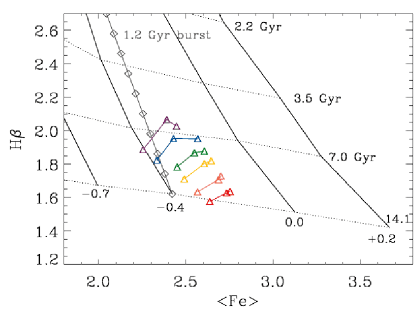
Figure 15.— Stellar population model grid showing the effect of adding a young burst to an underlying old population. The model grid is for a solar-scale abundance pattern model from Schiavon (2007). Solid (dotted) lines connect models with the same [Fe/H] (age). The gray track shows the effect of taking an old population with age = 14.1 Gyr and [Fe/H] = -0.4, and adding to it varying fractions of a 1.2 Gyr burst with the same [Fe/H]. Gray diamonds indicate the fraction of the total luminosity at 5000Å provided by the young burst, starting at 0% at the bottom and increasing in increments of 5%. Index values from the stacked spectra are overplotted as triangles, with colors indicating the $\sigma$ range of the stacked spectrum, as in Figure 3 (purple shows the lowest $\sigma$ bin, red the highest $\sigma$ bin). The three data points at fixed $\sigma$ show the three different bins in $L$. The age–[Fe/H] anticorrelation observed at fixed $\sigma$ cannot simply be due to the presence of a young sub-population in the brighter galaxies because the trajectory of a young burst at constant [Fe/H] is nearly orthogonal to the observed co-variation of $\langle$Fe$\rangle$ and H$\beta$ at fixed $\sigma$. The brighter galaxies must have higher average [Fe/H] than their faint counterparts at the same $\sigma$, in addition to having younger mean ages.

Appendix C

Table 2Properties of Galaxy Bins and Stacked Spectra

				Median	Median	Median
	$\sigma$ bin	$M_{r}$ bin	$g-r$ bin	$\log\sigma$	$M_{r}$	$(g-r)_{deV}$	Number	$S/N$
				(km s-1)	(mag)	(mag)		(Å-1)
1	$1.86<\log\sigma<2.00$	$-21.29<M_{r}<-20.49$	$0.665$–$0.697$	1.95	-20.76	0.685	52	149
2			$0.697$–$0.729$	1.97	-20.64	0.712	85	170
3			$0.729$–$0.761$	1.97	-20.65	0.741	57	128
4		$-20.49<M_{r}<-19.69$	$0.665$–$0.697$	1.94	-20.05	0.684	177	219
5			$0.697$–$0.729$	1.95	-20.08	0.713	390	325
6			$0.729$–$0.761$	1.95	-20.12	0.741	233	252
7		$-19.69<M_{r}<-18.89$	$0.665$–$0.697$	1.92	-19.40	0.685	55	113
8			$0.697$–$0.729$	1.94	-19.46	0.715	122	171
9			$0.729$–$0.761$	1.95	-19.46	0.740	63	130
10	$2.00<\log\sigma<2.09$	$-21.54<M_{r}<-20.74$	$0.680$–$0.712$	2.05	-20.94	0.699	81	189
11			$0.712$–$0.744$	2.07	-20.92	0.728	176	288
12			$0.744$–$0.776$	2.07	-20.95	0.753	87	188
13		$-20.74<M_{r}<-19.94$	$0.680$–$0.712$	2.05	-20.29	0.702	290	317
14			$0.712$–$0.744$	2.05	-20.32	0.727	724	511
15			$0.744$–$0.776$	2.06	-20.33	0.755	357	360
16		$-19.94<M_{r}<-19.14$	$0.680$–$0.712$	2.04	-19.75	0.702	93	158
17			$0.712$–$0.744$	2.05	-19.78	0.728	166	235
18			$0.744$–$0.776$	2.05	-19.76	0.753	80	164
19	$2.09<\log\sigma<2.18$	$-21.84<M_{r}<-21.04$	$0.693$–$0.725$	2.15	-21.31	0.713	170	355
20			$0.725$–$0.757$	2.15	-21.24	0.741	376	488
21			$0.757$–$0.789$	2.15	-21.23	0.768	142	287
22		$-21.04<M_{r}<-20.24$	$0.693$–$0.725$	2.13	-20.63	0.715	483	479
23			$0.725$–$0.757$	2.14	-20.63	0.741	1138	731
24			$0.757$–$0.789$	2.14	-20.61	0.767	552	507
25		$-20.24<M_{r}<-19.44$	$0.693$–$0.725$	2.12	-20.07	0.715	174	231
26			$0.725$–$0.757$	2.13	-20.05	0.740	376	367
27			$0.757$–$0.789$	2.13	-20.08	0.767	141	235
28	$2.18<\log\sigma<2.27$	$-22.23<M_{r}<-21.43$	$0.705$–$0.737$	2.23	-21.63	0.726	206	427
29			$0.737$–$0.769$	2.24	-21.62	0.753	398	568
30			$0.769$–$0.801$	2.24	-21.64	0.779	150	337
31		$-21.43<M_{r}<-20.63$	$0.705$–$0.737$	2.21	-21.05	0.727	420	520
32			$0.737$–$0.769$	2.22	-21.03	0.753	1057	844
33			$0.769$–$0.801$	2.23	-21.02	0.780	533	596
34		$-20.63<M_{r}<-19.83$	$0.705$–$0.737$	2.21	-20.36	0.728	221	301
35			$0.737$–$0.769$	2.22	-20.38	0.754	482	485
36			$0.769$–$0.801$	2.22	-20.44	0.779	166	283
37	$2.27<\log\sigma<2.36$	$-22.66<M_{r}<-21.86$	$0.718$–$0.750$	2.31	-22.11	0.741	138	385
38			$0.750$–$0.782$	2.32	-22.08	0.766	299	536
39			$0.782$–$0.814$	2.33	-22.05	0.790	111	334
40		$-21.86<M_{r}<-21.06$	$0.718$–$0.750$	2.29	-21.51	0.742	250	476
41			$0.750$–$0.782$	2.31	-21.48	0.766	671	785
42			$0.782$–$0.814$	2.32	-21.44	0.790	246	462
43		$-21.06<M_{r}<-20.26$	$0.718$–$0.750$	2.29	-20.72	0.743	113	258
44			$0.750$–$0.782$	2.30	-20.79	0.766	313	443
45			$0.782$–$0.814$	2.30	-20.82	0.791	149	325
46	$2.36<\log\sigma<2.50$	$-23.02<M_{r}<-22.22$	$0.732$–$0.764$	2.39	-22.37	0.757	45	242
47			$0.764$–$0.796$	2.40	-22.39	0.780	116	380
48			$0.796$–$0.828$	2.40	-22.46	0.803	52	257
49		$-22.22<M_{r}<-21.42$	$0.732$–$0.764$	2.38	-21.76	0.756	88	319
50			$0.764$–$0.796$	2.38	-21.86	0.781	228	497
51			$0.796$–$0.828$	2.40	-21.96	0.803	88	320
52		$-21.42<M_{r}<-20.62$	$0.732$–$0.764$	2.38	-21.11	0.755	54	218
53			$0.764$–$0.796$	2.38	-21.11	0.779	109	304
54			$0.796$–$0.828$	2.40	-21.06	0.810	38	187

Table 3Lick Indices and Stellar Population Properties of Stacked Spectra

	H$\beta$		$\langle$Fe$\rangle$		Mg $b$		Age		[Fe/H]		[Mg/H]		[Mg/Fe]
	(Å)		(Å)		(Å)		(Gyr)		(dex)		(dex)		(dex)
1	2.10 $\pm$	0.05	2.34 $\pm$	0.06	3.16 $\pm$	0.05	5.5 $\pm$	0.5	-0.22 $\pm$	0.03	-0.08 $\pm$	0.04	0.14 $\pm$	0.03
2	2.09 $\pm$	0.04	2.42 $\pm$	0.05	3.38 $\pm$	0.04	5.5 $\pm$	0.4	-0.16 $\pm$	0.03	-0.01 $\pm$	0.03	0.15 $\pm$	0.02
3	1.88 $\pm$	0.06	2.58 $\pm$	0.07	3.78 $\pm$	0.06	8.0 $\pm$	0.8	-0.12 $\pm$	0.03	0.03 $\pm$	0.05	0.15 $\pm$	0.03
4	2.17 $\pm$	0.03	2.39 $\pm$	0.04	2.99 $\pm$	0.03	5.0 $\pm$	0.3	-0.18 $\pm$	0.02	-0.11 $\pm$	0.03	0.07 $\pm$	0.02
5	2.07 $\pm$	0.03	2.35 $\pm$	0.03	3.20 $\pm$	0.03	6.0 $\pm$	0.4	-0.24 $\pm$	0.02	-0.10 $\pm$	0.03	0.14 $\pm$	0.02
6	1.96 $\pm$	0.03	2.43 $\pm$	0.04	3.41 $\pm$	0.03	7.1 $\pm$	0.4	-0.21 $\pm$	0.02	-0.07 $\pm$	0.03	0.14 $\pm$	0.02
7	1.98 $\pm$	0.06	2.24 $\pm$	0.07	2.88 $\pm$	0.06	7.5 $\pm$	0.9	-0.34 $\pm$	0.04	-0.25 $\pm$	0.05	0.09 $\pm$	0.04
8	1.89 $\pm$	0.04	2.23 $\pm$	0.05	3.14 $\pm$	0.04	8.7 $\pm$	0.7	-0.38 $\pm$	0.02	-0.22 $\pm$	0.03	0.16 $\pm$	0.02
9	1.80 $\pm$	0.06	2.30 $\pm$	0.06	3.41 $\pm$	0.05	10.3 $\pm$	1.1	-0.35 $\pm$	0.03	-0.17 $\pm$	0.05	0.18 $\pm$	0.05
10	2.16 $\pm$	0.04	2.49 $\pm$	0.04	3.34 $\pm$	0.04	4.8 $\pm$	0.3	-0.10 $\pm$	0.02	0.02 $\pm$	0.03	0.12 $\pm$	0.02
11	1.92 $\pm$	0.03	2.51 $\pm$	0.03	3.48 $\pm$	0.03	7.5 $\pm$	0.4	-0.17 $\pm$	0.02	-0.04 $\pm$	0.03	0.13 $\pm$	0.02
12	1.77 $\pm$	0.04	2.70 $\pm$	0.04	3.92 $\pm$	0.04	9.6 $\pm$	0.7	-0.09 $\pm$	0.04	0.03 $\pm$	0.05	0.12 $\pm$	0.02
13	2.07 $\pm$	0.03	2.35 $\pm$	0.03	3.18 $\pm$	0.03	5.9 $\pm$	0.4	-0.24 $\pm$	0.02	-0.10 $\pm$	0.03	0.14 $\pm$	0.02
14	1.96 $\pm$	0.02	2.47 $\pm$	0.03	3.44 $\pm$	0.03	7.1 $\pm$	0.3	-0.18 $\pm$	0.01	-0.05 $\pm$	0.02	0.13 $\pm$	0.01
15	1.82 $\pm$	0.03	2.47 $\pm$	0.03	3.61 $\pm$	0.03	9.1 $\pm$	0.5	-0.22 $\pm$	0.02	-0.05 $\pm$	0.03	0.17 $\pm$	0.02
16	1.85 $\pm$	0.05	2.33 $\pm$	0.05	3.10 $\pm$	0.04	9.3 $\pm$	0.8	-0.33 $\pm$	0.03	-0.24 $\pm$	0.04	0.09 $\pm$	0.03
17	1.85 $\pm$	0.03	2.30 $\pm$	0.04	3.42 $\pm$	0.03	9.3 $\pm$	0.6	-0.33 $\pm$	0.02	-0.13 $\pm$	0.03	0.20 $\pm$	0.02
18	1.77 $\pm$	0.05	2.37 $\pm$	0.05	3.56 $\pm$	0.05	10.3 $\pm$	0.9	-0.31 $\pm$	0.03	-0.11 $\pm$	0.04	0.20 $\pm$	0.03
19	2.05 $\pm$	0.02	2.58 $\pm$	0.02	3.60 $\pm$	0.02	5.6 $\pm$	0.3	-0.08 $\pm$	0.02	0.06 $\pm$	0.02	0.14 $\pm$	0.01
20	1.85 $\pm$	0.02	2.54 $\pm$	0.02	3.50 $\pm$	0.02	8.4 $\pm$	0.3	-0.17 $\pm$	0.01	-0.05 $\pm$	0.02	0.12 $\pm$	0.01
21	1.73 $\pm$	0.03	2.70 $\pm$	0.03	3.97 $\pm$	0.03	10.1 $\pm$	0.5	-0.11 $\pm$	0.01	0.03 $\pm$	0.03	0.14 $\pm$	0.02
22	2.00 $\pm$	0.02	2.49 $\pm$	0.02	3.59 $\pm$	0.02	6.6 $\pm$	0.3	-0.14 $\pm$	0.01	0.02 $\pm$	0.02	0.16 $\pm$	0.02
23	1.86 $\pm$	0.02	2.50 $\pm$	0.02	3.67 $\pm$	0.02	8.4 $\pm$	0.3	-0.18 $\pm$	0.01	-0.01 $\pm$	0.01	0.17 $\pm$	0.01
24	1.75 $\pm$	0.02	2.65 $\pm$	0.02	3.92 $\pm$	0.02	9.9 $\pm$	0.4	-0.13 $\pm$	0.01	0.02 $\pm$	0.02	0.15 $\pm$	0.02
25	1.87 $\pm$	0.03	2.29 $\pm$	0.04	3.39 $\pm$	0.03	8.7 $\pm$	0.6	-0.32 $\pm$	0.02	-0.12 $\pm$	0.03	0.20 $\pm$	0.02
26	1.82 $\pm$	0.03	2.57 $\pm$	0.03	3.83 $\pm$	0.03	9.0 $\pm$	0.4	-0.15 $\pm$	0.01	0.01 $\pm$	0.03	0.16 $\pm$	0.02
27	1.65 $\pm$	0.03	2.49 $\pm$	0.04	3.97 $\pm$	0.03	12.3 $\pm$	0.7	-0.26 $\pm$	0.02	-0.03 $\pm$	0.03	0.23 $\pm$	0.02
28	1.95 $\pm$	0.02	2.61 $\pm$	0.02	3.84 $\pm$	0.02	6.9 $\pm$	0.2	-0.06 $\pm$	0.01	0.11 $\pm$	0.02	0.17 $\pm$	0.02
29	1.79 $\pm$	0.01	2.65 $\pm$	0.02	3.84 $\pm$	0.01	9.2 $\pm$	0.2	-0.12 $\pm$	0.01	0.02 $\pm$	0.02	0.14 $\pm$	0.02
30	1.72 $\pm$	0.02	2.68 $\pm$	0.02	4.10 $\pm$	0.02	10.3 $\pm$	0.4	-0.11 $\pm$	0.01	0.07 $\pm$	0.02	0.18 $\pm$	0.02
31	1.91 $\pm$	0.02	2.53 $\pm$	0.02	3.78 $\pm$	0.02	7.5 $\pm$	0.2	-0.14 $\pm$	0.01	0.04 $\pm$	0.02	0.18 $\pm$	0.02
32	1.79 $\pm$	0.01	2.60 $\pm$	0.01	4.05 $\pm$	0.01	9.1 $\pm$	0.2	-0.13 $\pm$	0.01	0.08 $\pm$	0.01	0.21 $\pm$	0.01
33	1.70 $\pm$	0.01	2.69 $\pm$	0.02	4.23 $\pm$	0.01	10.6 $\pm$	0.3	-0.10 $\pm$	0.01	0.10 $\pm$	0.02	0.20 $\pm$	0.02
34	1.78 $\pm$	0.03	2.38 $\pm$	0.03	3.82 $\pm$	0.03	10.0 $\pm$	0.5	-0.28 $\pm$	0.01	-0.03 $\pm$	0.02	0.25 $\pm$	0.02
35	1.68 $\pm$	0.02	2.49 $\pm$	0.02	4.05 $\pm$	0.02	11.5 $\pm$	0.4	-0.24 $\pm$	0.01	0.02 $\pm$	0.02	0.26 $\pm$	0.02
36	1.67 $\pm$	0.03	2.60 $\pm$	0.03	4.28 $\pm$	0.03	11.3 $\pm$	0.5	-0.17 $\pm$	0.02	0.10 $\pm$	0.03	0.27 $\pm$	0.02
37	1.88 $\pm$	0.02	2.68 $\pm$	0.02	4.16 $\pm$	0.02	7.7 $\pm$	0.2	-0.03 $\pm$	0.01	0.17 $\pm$	0.01	0.20 $\pm$	0.01
38	1.71 $\pm$	0.01	2.71 $\pm$	0.02	4.27 $\pm$	0.01	10.2 $\pm$	0.2	-0.08 $\pm$	0.01	0.13 $\pm$	0.01	0.21 $\pm$	0.01
39	1.60 $\pm$	0.02	2.71 $\pm$	0.02	4.42 $\pm$	0.02	12.3 $\pm$	0.5	-0.12 $\pm$	0.01	0.12 $\pm$	0.02	0.24 $\pm$	0.01
40	1.80 $\pm$	0.02	2.65 $\pm$	0.02	4.14 $\pm$	0.02	8.8 $\pm$	0.2	-0.08 $\pm$	0.01	0.13 $\pm$	0.01	0.21 $\pm$	0.01
41	1.69 $\pm$	0.01	2.69 $\pm$	0.01	4.31 $\pm$	0.01	10.6 $\pm$	0.2	-0.10 $\pm$	0.01	0.12 $\pm$	0.02	0.22 $\pm$	0.02
42	1.62 $\pm$	0.02	2.72 $\pm$	0.02	4.46 $\pm$	0.02	11.8 $\pm$	0.3	-0.10 $\pm$	0.01	0.14 $\pm$	0.01	0.24 $\pm$	0.01
43	1.69 $\pm$	0.03	2.45 $\pm$	0.03	4.19 $\pm$	0.03	11.4 $\pm$	0.6	-0.25 $\pm$	0.02	0.06 $\pm$	0.03	0.31 $\pm$	0.02
44	1.64 $\pm$	0.02	2.58 $\pm$	0.02	4.33 $\pm$	0.02	11.9 $\pm$	0.4	-0.18 $\pm$	0.01	0.10 $\pm$	0.01	0.28 $\pm$	0.01
45	1.57 $\pm$	0.02	2.67 $\pm$	0.03	4.54 $\pm$	0.02	13.1 $\pm$	0.6	-0.14 $\pm$	0.01	0.13 $\pm$	0.02	0.27 $\pm$	0.02
46	1.67 $\pm$	0.03	2.73 $\pm$	0.03	4.48 $\pm$	0.03	10.9 $\pm$	0.6	-0.08 $\pm$	0.02	0.17 $\pm$	0.03	0.25 $\pm$	0.02
47	1.65 $\pm$	0.02	2.78 $\pm$	0.02	4.48 $\pm$	0.02	10.9 $\pm$	0.4	-0.05 $\pm$	0.01	0.19 $\pm$	0.02	0.23 $\pm$	0.02
48	1.59 $\pm$	0.03	2.74 $\pm$	0.03	4.69 $\pm$	0.03	12.2 $\pm$	0.6	-0.08 $\pm$	0.02	0.20 $\pm$	0.03	0.28 $\pm$	0.02
49	1.73 $\pm$	0.02	2.69 $\pm$	0.03	4.43 $\pm$	0.02	9.8 $\pm$	0.4	-0.07 $\pm$	0.01	0.18 $\pm$	0.03	0.25 $\pm$	0.02
50	1.56 $\pm$	0.01	2.70 $\pm$	0.02	4.56 $\pm$	0.01	13.0 $\pm$	0.4	-0.12 $\pm$	0.01	0.15 $\pm$	0.01	0.27 $\pm$	0.01
51	1.59 $\pm$	0.02	2.81 $\pm$	0.03	4.77 $\pm$	0.02	12.0 $\pm$	0.4	-0.04 $\pm$	0.01	0.23 $\pm$	0.02	0.27 $\pm$	0.02
52	1.61 $\pm$	0.04	2.57 $\pm$	0.04	4.48 $\pm$	0.03	12.7 $\pm$	0.8	-0.19 $\pm$	0.02	0.12 $\pm$	0.03	0.31 $\pm$	0.02
53	1.58 $\pm$	0.03	2.65 $\pm$	0.03	4.62 $\pm$	0.02	12.8 $\pm$	0.6	-0.14 $\pm$	0.01	0.16 $\pm$	0.03	0.30 $\pm$	0.02
54	1.54 $\pm$	0.04	2.69 $\pm$	0.04	4.80 $\pm$	0.04	13.4 $\pm$	1.0	-0.12 $\pm$	0.02	0.20 $\pm$	0.03	0.32 $\pm$	0.03

References

- Adelman-McCarthy et al. (2006) Adelman-McCarthy, J. K., et al. 2006, ApJS, 162, 38
- Adelman-McCarthy (2007) Adelman-McCarthy, J. K., et al. 2007, ArXiv e-prints, 707
- Baldwin et al. (1981) Baldwin, J. A., Phillips, M. M., & Terlevich, R. 1981, PASP, 93, 5
- Bender et al. (1993) Bender, R., Burstein, D., & Faber, S. M. 1993, ApJ, 411, 153
- Bernardi (2007) Bernardi, M. 2007, AJ, 133, 1954
- Bernardi et al. (2007) Bernardi, M., Hyde, J. B., Sheth, R. K., Miller, C. J., & Nichol, R. C. 2007, AJ, 133, 1741
- Bernardi et al. (2003a) Bernardi, M., et al. 2003a, AJ, 125, 1817
- Bernardi et al. (2003b) Bernardi, M., et al. 2003b, AJ, 125, 1882
- Bernardi et al. (2005) Bernardi, M., Sheth, R. K., Nichol, R. C., Schneider, D. P., & Brinkmann, J. 2005, AJ, 129, 61
- Blanton et al. (2003) Blanton, M. R., et al. 2003, AJ, 125, 2348
- Blanton et al. (2001) Blanton, M. R., et al. 2001, AJ, 121, 2358
- Blanton et al. (2005) Blanton, M. R., et al. 2005, AJ, 129, 2562
- Bower et al. (1992) Bower, R. G., Lucey, J. R., & Ellis, R. S. 1992, MNRAS, 254, 601
- Burbidge et al. (1961) Burbidge, E. M., Burbidge, G. R., & Fish, R. A. 1961, ApJ, 133, 393
- Burstein et al. (1984) Burstein, D., Faber, S. M., Gaskell, C. M., & Krumm, N. 1984, ApJ, 287, 586
- Cardiel et al. (1998) Cardiel, N., Gorgas, J., Cenarro, J., & Gonzalez, J. J. 1998, A&AS, 127, 597
- Colless et al. (1999) Colless, M., Burstein, D., Davies, R. L., McMahan, R. K., Saglia, R. P., & Wegner, G. 1999, MNRAS, 303, 813
- Cool et al. (2006) Cool, R. J., Eisenstein, D. J., Johnston, D., Scranton, R., Brinkmann, J., Schneider, D. P., & Zehavi, I. 2006, AJ, 131, 736
- Djorgovski & Davis (1987) Djorgovski, S. & Davis, M. 1987, ApJ, 313, 59
- Dressler et al. (1987) Dressler, A., Lynden-Bell, D., Burstein, D., Davies, R. L., Faber, S. M., Terlevich, R., & Wegner, G. 1987, ApJ, 313, 42
- Faber (1973) Faber, S. M. 1973, ApJ, 179, 731
- Faber et al. (1987) Faber, S. M., Dressler, A., Davies, R. L., Burstein, D., & Lynden-Bell, D. 1987, in Nearly Normal Galaxies: From the Planck Time to the Present, ed. S. M. Faber, 175–183
- Faber & Jackson (1976) Faber, S. M. & Jackson, R. E. 1976, ApJ, 204, 668
- Faber et al. (1995) Faber, S. M., Trager, S. C., Gonzalez, J. J., & Worthey, G. 1995, in IAU Symposium, Vol. 164, Stellar Populations, ed. P. C. van der Kruit & G. Gilmore, 249
- Fukugita et al. (1996) Fukugita, M., Ichikawa, T., Gunn, J. E., Doi, M., Shimasaku, K., & Schneider, D. P. 1996, AJ, 111, 1748
- Fulbright et al. (2007) Fulbright, J. P., McWilliam, A., & Rich, R. M. 2007, ApJ, 661, 1152
- Gallazzi et al. (2006) Gallazzi, A., Charlot, S., Brinchmann, J., & White, S. D. M. 2006, MNRAS, 370, 1106
- Gallazzi et al. (2005) Gallazzi, A., Charlot, S., Brinchmann, J., White, S. D. M., & Tremonti, C. A. 2005, MNRAS, 362, 41
- Girardi et al. (2000) Girardi, L., Bressan, A., Bertelli, G., & Chiosi, C. 2000, A&AS, 141, 371
- Gladders & Yee (2000) Gladders, M. D. & Yee, H. K. C. 2000, AJ, 120, 2148
- Graves et al. (2007) Graves, G. J., Faber, S. M., Schiavon, R. P., & Yan, R. 2007, ApJ, 671, 243
- Graves & Schiavon (2008) Graves, G. J. & Schiavon, R. P. 2008, ArXiv e-prints, 802
- Gunn et al. (1998) Gunn, J. E., et al. 1998, AJ, 116, 3040
- Gunn et al. (2006) Gunn, J. E., et al. 2006, AJ, 131, 2332
- Hogg et al. (2001) Hogg, D. W., Finkbeiner, D. P., Schlegel, D. J., & Gunn, J. E. 2001, AJ, 122, 2129
- Humphrey & Buote (2006) Humphrey, P. J. & Buote, D. A. 2006, ApJ, 639, 136
- Ivezić et al. (2004) Ivezić, Ž., et al. 2004, Astronomische Nachrichten, 325, 583
- Jones (1999) Jones, C. D. 1999, PhD thesis, Univ. of Washington
- Jørgensen (1999) Jørgensen, I. 1999, MNRAS, 306, 607
- Jørgensen et al. (1995) Jørgensen, I., Franx, M., & Kjaergaard, P. 1995, MNRAS, 276, 1341
- Kauffmann et al. (2003) Kauffmann, G., et al. 2003, MNRAS, 346, 1055
- Kelson et al. (2006) Kelson, D. D., Illingworth, G. D., Franx, M., & van Dokkum, P. G. 2006, ApJ, 653, 159
- Kodama & Arimoto (1997) Kodama, T. & Arimoto, N. 1997, A&A, 320, 41
- Kormendy (1985) Kormendy, J. 1985, ApJ, 295, 73
- Korn et al. (2005) Korn, A. J., Maraston, C., & Thomas, D. 2005, A&A, 438, 685
- Kuntschner & Davies (1998) Kuntschner, H. & Davies, R. L. 1998, MNRAS, 295, L29
- Kuntschner et al. (2001) Kuntschner, H., Lucey, J. R., Smith, R. J., Hudson, M. J., & Davies, R. L. 2001, MNRAS, 323, 615
- Lauer (1985) Lauer, T. R. 1985, ApJ, 292, 104
- Lauer et al. (2007) Lauer, T. R., et al. 2007, ApJ, 662, 808
- Lisker et al. (2007) Lisker, T., Grebel, E. K., Binggeli, B., & Glatt, K. 2007, ApJ, 660, 1186
- Lupton et al. (2001) Lupton, R., Gunn, J. E., Ivezić, Z., Knapp, G. R., & Kent, S. 2001, in Astro. Soc. of the Pacific Conf. Ser., Vol. 238, ed. F. R. Harnden, Jr., F. A. Primini, & H. E. Payne, 269
- Nelan et al. (2005) Nelan, J. E., Smith, R. J., Hudson, M. J., Wegner, G. A., Lucey, J. R., Moore, S. A. W., Quinney, S. J., & Suntzeff, N. B. 2005, ApJ, 632, 137
- Noeske et al. (2007) Noeske, K. G., et al. 2007, ApJ, 660, L47
- Pier et al. (2003) Pier, J. R., Munn, J. A., Hindsley, R. B., Hennessy, G. S., Kent, S. M., Lupton, R. H., & Ivezić, Ž. 2003, AJ, 125, 1559
- Poggianti et al. (2001) Poggianti, B. M., et al. 2001, ApJ, 562, 689
- Rix & White (1992) Rix, H.-W. & White, S. D. M. 1992, MNRAS, 254, 389
- Sandage & Visvanathan (1978) Sandage, A. & Visvanathan, N. 1978, ApJ, 223, 707
- Schawinski et al. (2007) Schawinski, K., Thomas, D., Sarzi, M., Maraston, C., Kaviraj, S., Joo, S.-J., Yi, S. K., & Silk, J. 2007, MNRAS, 382, 1415
- Schiavon (2007) Schiavon, R. P. 2007, ApJS, 171, 146
- Smith et al. (2002) Smith, J. A., et al. 2002, AJ, 123, 2121
- Smith et al. (2007a) Smith, R. J., Lucey, J. R., & Hudson, M. J. 2007a, MNRAS, 381, 1035
- Smith et al. (2007b) —. 2007b, ArXiv e-prints, 712
- Stoughton et al. (2002) Stoughton, C., et al. 2002, Proceedings of the SPIE Vol. 4836, ed. Tyson, J. A.; & Wolff, S., 339–349
- Strauss et al. (2002) Strauss, M. A., et al. 2002, AJ, 124, 1810
- Terlevich & Forbes (2002) Terlevich, A. I. & Forbes, D. A. 2002, MNRAS, 330, 547
- Thomas et al. (2005) Thomas, D., Maraston, C., Bender, R., & Mendes de Oliveira, C. 2005, ApJ, 621, 673
- Tinsley (1981) Tinsley, B. M. 1981, MNRAS, 194, 63
- Trager et al. (2008) Trager, S. C., Faber, S. M., & Dressler, A. 2008, MNRAS, 441
- Trager et al. (2000) Trager, S. C., Faber, S. M., Worthey, G., & González, J. J. 2000, AJ, 120, 165
- Trager et al. (1998) Trager, S. C., Worthey, G., Faber, S. M., Burstein, D., & Gonzalez, J. J. 1998, ApJS, 116, 1
- Tucker et al. (2006) Tucker, D. L., et al. 2006, Astronomische Nachrichten, 327, 821
- Worthey (1994) Worthey, G. 1994, ApJS, 95, 107
- Worthey et al. (1994) Worthey, G., Faber, S. M., Gonzalez, J. J., & Burstein, D. 1994, ApJS, 94, 687
- Worthey & Ottaviani (1997) Worthey, G. & Ottaviani, D. L. 1997, ApJS, 111, 377
- Worthey et al. (1995) Worthey, G., Trager, S. C., & Faber, S. M. 1995, in Astro. Soc. of the Pacific Conf. Ser., Vol. 86, ed. A. Buzzoni, A. Renzini, & A. Serrano, 203
- Yan et al. (2006) Yan, R., Newman, J. A., Faber, S. M., Konidaris, N., Koo, D., & Davis, M. 2006, ApJ, 648, 281
- York et al. (2000) York, D. G., et al. 2000, AJ, 120, 1579