Gaussian wave packets in phase space: The Fermi $g_{F}$ function

Abstract

Any pure quantum state can be equivalently represented by means of its wave function $\psi(q)$ or of the Fermi function $g_{F}(q,p)$, with $q$ and $p$ coordinates and conjugate momenta of the system under investigation. We show that a Gaussian wave packet can be conveniently visualized in phase space by means of the curve $g_{F}(q,p)=0$. The evolution in time of the $g_{F}=0$ curve is then computed for a Gaussian packet evolving freely or under a constant or a harmonic force. As a result, the spreading or shrinking of the packet is easily interpreted in phase space. Finally, we discuss a gedanken prism microscope experiment for measuring the position-momentum correlation. This gedanken experiment, together with the well-known Heisenberg microscope and von Neumann velocimeter, is sufficient to fully determine the state of a Gaussian packet.

I Introduction

The free propagation of a Gaussian wave packet is the simplest application of the time-dependent Schrödinger equation. In their first quantum mechanics course, students soon learn that, for a free particle, a minimum-uncertainty Gaussian packet spreads in time. They also learn that, for a harmonic oscillator, such minimum packet does not spread. Since, according to the Ehrenfest theorem, a quantum wave packet follows a beam of classical orbits as long as the packet remains narrow, one can conclude that the harmonic motion of a minimum packet can be described by means of classical mechanics.

On the other hand, it should be stressed that:

(i) If we call $q$ and $p$ the coordinate and momentum of the system under investigation, then also a beam of classical orbits can spread along $q$. That is, the spreading is not necessarily a quantum phenomenon.

(ii) Gaussian wave packets can also contract along $q$, namely the position uncertainty can narrow along $q$. Given an arbitrarily long time $\tau$, it is possible to build packets that shrink up to that time. klein

Heisenberg uncertainty principle forbids the notion of trajectories in quantum mechanics. However, a comparison between classical and quantum dynamics can be made by studying the evolution in time of the classical and quantum phase space distributions. lee ; heller ; qcbook2 ; brumer ; zurek ; davidovich ; habib The classical phase space distribution $\rho_{C}(q,p,t)$ determines the probability $\rho_{C}(q,p,t)\,dq\,dp$ that a particle is found at time $t$ in the infinitesimal phase space volume $dq\,dp$ centered at $(q,p)$. The evolution in time of $\rho$ is governed by the Liouville’s equation. goldstein A convenient phase space formulation of quantum mechanics is obtained using the Wigner distribution function $\rho_{W}(q,p,t)$. wigner ; wignerreview Such distribution evolves according to a quantum Liouville equation. However, the Wigner function in general is not positive definite and therefore requires the introduction of delicate concepts such as that of quasiprobability.

In this paper, we follow a different phase space approach, based on an old paper by Fermi. fermi The relevant quantity here is the Fermi $g_{F}$ function, or more precisely the $g_{F}(q,p,t)=0$ curve. We will show that the $g_{F}$ function provides a nice intuitive phase space picture of Gaussian wave packets and of their evolution in time. In particular, the spreading or shrinking of a Gaussian packet evolving freely or under a constant or a harmonic force are easily interpreted in the Fermi-function picture. Finally, we will discuss gedanken experiments determining the $g_{F}=0$ Fermi curve for Gaussian packets. In particular, we will focus on a prism microscope capable of measuring the position-momentum correlation. It turns out that the prism microscope, together with the well-known Heisenberg microscope and von Neumann’s velocimeter, fully determines the $g_{F}=0$ curve for Gaussian packets.

II The Fermi $g_{F}$ function

For the sake of simplicity, we consider the case of a single particle moving along a straight line. In classical mechanics, it is possible to determine the state of such system by measuring at some time $t$ the values of the position $q$ and momentum $p$ or, equivalently, by measuring two independent functions $f(q,p)$ and $g(q,p)$, from which the values of $q$ and $p$ can be obtained.

In quantum mechanics, due to Heisenberg uncertainty principle, a simultaneous exact measurement of $q$ and $p$ is not possible. An exact measurement is in principle possible only for one physical quantity: $q$ or $p$ or any function $g(q,p)$. Of course different choices of $g(q,p)$ lead to different determinations of the system. For instance, an exact measurement of $q$ implies a complete indetermination of $p$, and vice versa.

As pointed out by Fermi, fermi the state of a quantum system at a given time $t$ may be defined in two completely equivalent ways: (i) by its wave function $\psi(q,t)$ or (ii) by measuring a physical quantity $g_{F}(q,p,t)$. Indeed, given the measurement outcome $g_{F}(q,p,t)=\bar{g}$, then $\psi(q,t)$ is obtained as solution of the eigenvalue equation $g_{F}(q,p,t)\psi(q,t)=\bar{g}\psi(q,t)$, where $p=-i\hbar{\partial_{q}}$. On the other hand, given the wave function $\psi(q,t)$ it is always possible to find an operator $g_{F}(q,p,t)$ such that

$$g_{F}(q,p,t)\psi(q,t)=0.$$ (1)

Using the polar decomposition

$$\psi(q,t)=\rho(q,t)e^{i\theta(q,t)},$$ (2)

where $\rho$ and $\theta$ are real ($\rho\geq 0$), it is easy to check that identity (1) is indeed fulfilled by taking

$${g}_{F}\left(q,-i\hbar\partial_{q},t\right)=\left[-i\hbar\partial_{q}-\hbar\partial_{q}\theta(q,t)\right]^{2}+\hbar^{2}\frac{\partial_{qq}^{2}\rho(q,t)}{\rho(q,t)}.$$ (3)

Equation (1) implies that the corresponding physical quantity $g_{F}(q,p,t)$ takes the value $\bar{g}=0$. Therefore, the equation

$$g_{F}(q,p,t)=\left[p-\hbar\partial_{q}\theta(q,t)\right]^{2}+\hbar^{2}\frac{\partial_{qq}^{2}\rho(q,t)}{\rho(q,t)}=0$$ (4)

defines a curve in the two-dimensional phase space, parametrically dependent on time $t$. In other words, as expected from Heisenberg uncertainty principle, we cannot identify a quantum particle by means of a point $(q,p)$ but we need a curve $g_{F}(q,p,t)=0$. We call $g_{F}$ the Fermi function and we are interested in the phase space curve $g_{F}=0$. It is also possible to write equation (4) in the form

$$p_{\pm}=\hbar\partial_{q}\theta(q,t)\pm\sqrt{-\hbar^{2}\frac{\partial_{qq}^{2}\rho(q,t)}{\rho(q,t)}}.$$ (5)

This equation locates two points $(q,p_{+})$ and $(q,p_{-})$ in the phase space for any $q$ such that $\partial_{qq}^{2}\rho(q,t)<0$ and $\rho(q,t)\neq 0$. footnote

III The Fermi $g_{F}$ function for Gaussian wave packets

In this section, we discuss the phase space curve $g_{F}(q,p,t)=0$ corresponding to the wave function $\psi(q,t)$ solution to the one-dimensional Schrödinger equation

$$i\hbar\partial_{t}\psi(q,t)=\left[-\frac{\hbar^{2}}{2m}{\partial_{qq}^{2}}+V(q)\right]\psi(q,t),$$ (6)

for various time-independent potentials $V(q)$ such that an initially Gaussian wave packet $\psi(q,0)$ remains Gaussian at all times.

III.1 Free particle

We have $V(q)=0$ and consider as initial condition the Gaussian minimum uncertainty wave packet

$$\psi(q,0)=\frac{1}{\sqrt{\sqrt{\pi}\delta}}\exp\left\{-\frac{(q-q_{0})^{2}}{2\delta^{2}}+\frac{i}{\hbar}[p_{0}(q-q_{0})]\right\}.$$ (7)

The solution to the Schrödinger equation (6) with this initial condition reads

$$\begin{array}[]{c}{\displaystyle\psi(q,t)=\frac{1}{\sqrt{\sqrt{\pi}\left(1+i\frac{\hbar t}{m\delta^{2}}\right)\delta}}\exp\left\{-\frac{\left(q-q_{0}-\frac{p_{0}t}{m}\right)^{2}}{2\delta^{2}\left(1+i\frac{\hbar t}{m\delta^{2}}\right)}\right.}\\ \\ {\displaystyle\left.+\frac{i}{\hbar}\left[p_{0}(q-q_{0})-\frac{p_{0}^{2}t}{2m}\right]\right\}.}\end{array}$$ (11)

We now apply operator (3) to this wave function, thus obtaining

$$f(t)g_{F}(q,p,t)=\frac{\tilde{q}^{2}}{\delta^{2}}+\frac{\delta^{2}}{\hbar^{2}}\left(1+\frac{\hbar^{2}t^{2}}{m^{2}\delta^{4}}\right)\tilde{p}^{2}-\frac{2t}{m\delta^{2}}\tilde{q}\tilde{p}-1,$$ (12)

where for later convenience we have multiplied the Fermi function by $f(t)=\frac{\delta^{2}}{\hbar^{2}}\left(1+\frac{\hbar^{2}t^{2}}{m^{2}\delta^{4}}\right)$ and we have defined

$$\tilde{q}=q-q_{0}-\frac{p_{0}t}{m},\quad\tilde{p}=p-p_{0}.$$ (13)

The $g_{F}(q,p,t)=0$ curve is the ellipse

$$a\tilde{q}^{2}+b\tilde{p}^{2}+2c\tilde{q}\tilde{p}=1,$$ (14)

where

$$a=\frac{1}{\delta^{2}},\quad b=\frac{\delta^{2}}{\hbar^{2}}\left(1+\frac{\hbar^{2}t^{2}}{m^{2}\delta^{4}}\right),\quad c=-\frac{t}{m\delta^{2}}.$$ (15)

As shown in Fig. 1, the shape of the ellipse changes over time. However, its area

$$A=\frac{\pi}{\sqrt{ab-c^{2}}}=\pi\hbar$$ (16)

remains constant.

Figure 1: Phase space curves $g_{F}=0$ at different times (from left to right, $\tau=\frac{\hbar t}{m\delta^{2}}=-3,-2,-1,0,1,2,3$) for a free particle, whose state at $t=0$ is a minimum uncertainty Gaussian wave packet centered at $\left(\frac{q_{0}}{\delta}=0,\frac{\delta p_{0}}{\hbar}=2\right)$.

III.2 Uniformly accelerating particle

We have $V(q)=-F_{0}q$. In this case, the solution to the Schrödinger equation (6) with initial condition the Gaussian minimum uncertainty wave packet (7) reads

$$\begin{array}[]{c}{\displaystyle\psi(q,t)=}\\ {\displaystyle\frac{1}{\sqrt{\sqrt{\pi}\left(1+i\frac{\hbar t}{m\delta^{2}}\right)\delta}}\exp\left\{-\frac{\left(q-q_{0}-\frac{p_{0}t}{m}-\frac{F_{0}t^{2}}{2m}\right)^{2}}{2\delta^{2}\left(1+i\frac{\hbar t}{m\delta^{2}}\right)}\right.}\\ \\ {\displaystyle\left.+\frac{i}{\hbar}\left[p_{0}(q-q_{0})-\frac{p_{0}^{2}}{2m}t+\phi\right]\right\},}\end{array}$$ (21)

where

$$\phi=F_{0}qt-\frac{F_{0}p_{0}t^{2}}{2m}-\frac{F_{0}^{2}t^{3}}{6m}.$$ (22)

The Fermi $g_{F}$ function is again given by equation (12), but with the center of the ellipse accelerating uniformly, namely we have

$$\tilde{q}=q-q_{0}-\frac{p_{0}t}{m}-\frac{F_{0}t^{2}}{2m},\quad\tilde{p}=p-p_{0}-F_{0}t.$$ (23)

The deformation with time of the ellipse $g_{F}=0$ is independent of the force $F_{0}$, which simply displaces the center $(\tilde{q},\tilde{p})$ of the ellipse along the parabola

$$q=q_{0}+\frac{p_{0}}{mF_{0}}(p-p_{0})+\frac{(p-p_{0})^{2}}{2mF_{0}}.$$ (24)

The curves $g_{F}=0$ at different times are shown in Fig. 2.

Figure 2: Same as in Fig. 1, but for a uniformly accelerating particle with $\frac{m\delta^{3}F_{0}}{\hbar^{2}}=1.5$. The $t=0$ minimum uncertainty Gaussian wave packet is centered at $\left(\frac{q_{0}}{\delta}=0,\frac{\delta p_{0}}{\hbar}=0\right)$.

III.3 Harmonic oscillator

We have $V(q)=\frac{1}{2}m\omega_{0}^{2}q^{2}$. A Gaussian solution to the Schrödinger equation (6) is given by

$$\psi(q,t)=N(t)\exp\left\{-\frac{1}{2}A(t)[q-Q(t)]^{2}+i\chi(q,t)\right\},$$ (25)

where

$$N(t)=\sqrt{\frac{\alpha}{\sqrt{\pi}}}\frac{1}{\sqrt{C(t)+i\sqrt{B}S(t)}},$$ (26)

$$C(t)=\cos(\omega_{0}t+\phi),\;S(t)=\sin(\omega_{0}t+\phi),\;B=\frac{\hbar^{2}\alpha^{4}}{m^{2}\omega_{0}^{2}},$$ (27)

$$A(t)=A_{r}(t)+iA_{i}(t),$$ (28)

$$A_{r}(t)=\frac{m\omega_{0}\sqrt{B}}{\hbar[C^{2}(t)+BS^{2}(t)]},$$ (29)

$$A_{i}(t)=\frac{m\omega_{0}(1-B)C(t)S(t)}{\hbar[C^{2}(t)+BS^{2}(t)]},$$ (30)

$$Q(t)=Q_{0}C(t),$$ (31)

$$\chi(q,t)=-\frac{\omega_{0}m}{\hbar}Q_{0}qS(t)+\frac{m\omega_{0}}{2\hbar}Q_{0}^{2}C(t)S(t).$$ (32)

Different values of the parameters $\alpha$, $Q_{0}$ and $\phi$ correspond to different solutions to the Schrödinger equation. Note that, for the sake of simplicity, we have not considered in (25) the most general Gaussian wave packet for the harmonic oscillator. dodonov

Due to the time dependence of $A(t)$, it is not immediate to grasp the evolution of the Gaussian packet (25). A clear illustration is provided by the Fermi function. The $g_{F}(q,p,t)=0$ curve is derived from equation (4) and again is a (parametrically dependent on $t$) ellipse in phase space, whose equation can be written in the form (14), with

$$a=\frac{A_{r}^{2}+A_{i}^{2}}{A_{r}},\quad b=\frac{1}{\hbar^{2}A_{r}},\quad c=\frac{A_{i}}{\hbar A_{r}},$$ (33)

$$\tilde{q}=q-Q(t),\quad\tilde{p}=p-m\dot{Q}(t).$$ (34)

Note that the area of the ellipse remains constant: $A=\pi\hbar$. Owing to the term proportional to $\tilde{q}\tilde{p}$, the ellipse in general does not have its axes parallel to the coordinate axes $q,p$. This term disappears when $A_{i}=0$, that is, for $B=1$ ($\alpha^{2}=\frac{m\omega_{0}}{\hbar}$). This special case corresponds to coherent states, for which the $g_{F}=0$ curve becomes, in the coordinate plane $\left(q,\frac{p}{m\omega_{0}}\right)$, a rigidly moving circle:

$$[q-Q(t)]^{2}+\frac{[p-m\dot{Q}(t)]^{2}}{m^{2}\omega_{0}^{2}}=\frac{\hbar}{m\omega_{0}}.$$ (35)

A more generic example (squeezed state) is shown in Fig. 3.

Figure 3: Same as in Fig. 1, but for the squeezed state (25) of a harmonic oscillator, with $\frac{m\omega_{0}Q_{0}^{2}}{\hbar}=20$, $B=0.1$ and $\omega_{0}t+\phi$ ranging from $0$ to $7\pi/4$, in steps of $\pi/4$.

IV Measuring the position-momentum correlation: A gedanken experiment

It is easy to check that, for the examples discussed above, the evolution of the phase space region enclosed by the $g_{F}(q,p,t)=0$ curve is the same as for the corresponding classical phase space distribution $\rho_{C}(q,p,t)$, uniform inside such region and zero-valued outside and evolving according to the Liouville equation. Due to this equivalence, the conservation of the area of this region is assured by the Liouville theorem. goldstein However, we should stress that the spreading or the shrinking of a wave packet are quantum effects, in the sense that the wave packet refers to a single particle, while the distribution function $\rho_{C}(q,p,t)$ describes a classical ensemble of orbits. No physical meaning should be attached to each point inside the $g_{F}=0$ curve. Due to Heisenberg principle it is not possible to assign with arbitrarily small uncertainties both position and momentum.

For Gaussian states, the area enclosed by the Fermi $g_{F}$ function has a simple interpretation in terms of Heisenberg uncertainty principle. To illustrate this point, let us compute the variances

$$(\Delta q)^{2}=\langle(q-\langle q\rangle)^{2}\rangle,\quad(\Delta p)^{2}=\langle(p-\langle p\rangle)^{2}\rangle$$ (36)

and the position-momentum correlation

$$K=\frac{1}{2}\langle(q-\langle q\rangle)(p-\langle p\rangle)+(p-\langle p\rangle)(q-\langle q\rangle)\rangle$$ (37)

for the examples discussed in the previous section. In the case of a free or uniformly accelerating particle we obtain

$$(\Delta q)^{2}=\frac{\delta^{2}}{2}\left(1+\frac{\hbar^{2}t^{2}}{m^{2}\delta^{4}}\right),\;(\Delta p)^{2}=\frac{\hbar^{2}}{2\delta^{2}},\;K=\frac{\hbar^{2}t}{2m\delta^{2}},$$ (38)

while for the harmonic oscillator

$$\begin{array}[]{c}{\displaystyle(\Delta q)^{2}=\frac{1}{2A_{r}},\;(\Delta p)^{2}=\frac{\hbar^{2}(A_{r}^{2}+A_{i}^{2})}{2A_{r}},}\\ {\displaystyle K=-\frac{\hbar(1-B)CS}{2\sqrt{B}}.}\end{array}$$ (39)

In both cases, the generalized uncertainty relation robertson ; dodonov ; sudarshan

$$(\Delta q)^{2}(\Delta p)^{2}-K^{2}=\frac{\hbar^{2}}{4}$$ (40)

is fulfilled. Moreover, the parameters determining the $g_{F}=0$ ellipse can be expressed as follows: $a=\frac{2}{\hbar^{2}}(\Delta p)^{2}$, $b=\frac{2}{\hbar^{2}}(\Delta q)^{2}$ and $c=\frac{2}{\hbar^{2}}K$ (for the free or uniformly accelerating particle) or $c=-\frac{2}{\hbar^{2}}K$ (for the harmonic oscillator). This implies that in these examples the experimental determination of the $g_{F}=0$ ellipse is possible once the quantities $\langle q\rangle$, $(\Delta q)^{2}$, $\langle p\rangle$, $(\Delta p)^{2}$ and $K$ are measured.

A simple consequence is that the spreading (in $q$) of a Gaussian wave packet for a free or uniformly accelerating particle as well as the oscillations in time of the $q$ and $p$ variances for a harmonic oscillator can be simply visualized in terms of the evolution in time of the $g_{F}=0$ curve or, equivalently, of the phase space region enclosed by this curve. We stress that here the conservation of the area of the $g_{F}=0$ ellipse is equivalent to the validity of the generalized uncertainty relation (40) at all times. The product $\Delta q\Delta p$ may grow or even reduce in time. This can be clearly seen from Figs. 1 and 2: $\Delta q\Delta p$ grows if we start from a minimum uncertainty state; on the other hand, if we start from a different state, $\Delta q\Delta p$ may decrease until the minimum uncertainty state is reached and then starts growing.

Notwithstanding the behaviour of $\Delta q\Delta p$, the uncertainty in the measurement of the state in phase space is constant, provided that we measure not only position and momentum but also their correlation $K$. For the complete determination of the $g_{F}=0$ ellipse we need three thought experiments:

(i) The measurement of $\langle q\rangle$ and $(\Delta q)^{2}$. This can be done by means of Heisenberg microscope.

(ii) The mesurement of $\langle p\rangle$ and $(\Delta p)^{2}$, possible using von Neumann velocimeter.

(iii) The measurement of the position-momentum correlator $K$.

The first two gedanken experiments are well known and their description can be found, for instance, in Ref. vonNeumann . In order to measure the correlator $K$, one can use Heisenberg microscope with the addition of a prism after the objective, grassistrini see Fig. 4.

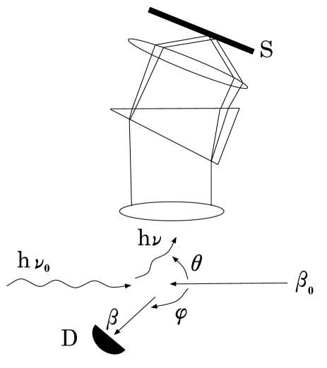
Figure 4: Schematic drawing of a thought microscope, measuring the position-momentum correlation of a particle. The scattered light is collected on the screen $S$. Note that a coincidence system with the detector $D$ of the scattered particle is necessary, in order to fix the scattering angle.

The main idea of this prism microscope gedanken experiment is suggested by the objective prism spectroscopy used for astronomical spectroscopy. In that case, a prism is placed in front of the objective lens of a telescope. As a result, the light coming from stars within the field of view of the telescope is dispersed by the prism depending on its frequency. Therefore, the telescope can be used for simultaneously measuring the spectra of many stars. physicstoday In our case, the prism is located after the lens of the microscope (see Fig. 4), so that, if the refractive index of the prism is a suitable function of the wave length of the scattered photon, then such photon strikes the screen $S$ in a position dependent of the position-momentum correlation of the measured particle.

We now sketch the working of the prism microscope. We first write the equations of the Compton effect for the scattering between the photon (our probe) and the measured particle. Considering a scattering event on the plane of Fig. 4, the nonrelativistic energy-momentum conservation laws read as follows:

$$\left\{\begin{array}[]{l}\displaystyle h\nu_{0}+\frac{1}{2}mc^{2}\beta_{0}^{2}=h\nu+\frac{1}{2}mc^{2}\beta^{2},\\ \displaystyle h\nu_{0}-m\beta_{0}c^{2}=h\nu\cos\theta+m\beta c^{2}\cos\varphi,\\ \displaystyle h\nu\sin\theta-m\beta c^{2}\sin\varphi=0,\end{array}\right.$$ (41)

where $h$ is Planck constant, $c$ the speed of light in vacuum, $m$ the particle mass, $\nu_{0}$ and $\nu$ ($\beta_{0}c$ and $\beta c$) denote the photon frequency (the particle velocity) before and after the collision, $\theta$ and $\varphi$ are the scattering angles.

There are five unknown parameters in the Compton scattering equations (41): $\nu,\beta_{0},\beta,\theta,\varphi$. If we fix $\varphi$ and exploit (41), then we can obtain a single equation $F(\nu,\beta_{0})=0$ that relates the frequency $\nu$ of the scattered light to the velocity $c\beta_{0}$ of the particle. By linearizing such equation we obtain

$$\nu\approx A+B(\beta_{0}-\langle\beta_{0}\rangle),$$ (42)

with $A,B$ constants and $c\langle\beta_{0}\rangle$ mean value of the particle velocity. It is clear that, in order to fix the angle $\varphi$, a coincidence system between the detector measuring the angle $\varphi$ of the scattered particle and the screen is needed.

If the refractive index of the prism is a suitable and known function of the frequency $\nu$ of the scattered light and assuming that linearization (42) holds, then we collect on a screen a spot whose location depends on the position-momentum correlation of the measured particle. If without the prism the photon hits the screen at the position $\xi=q$, then with the prism $\xi$ is displaced by an amount depending on the frequency $\nu$. If the refractive index is a linear function of $\nu$, then we obtain $\xi=q+Cp$, with $C$ constant. Considering a more generic suitable nonlinear dependence of the refractive index on $\nu$, we obtain

$$\xi\approx q+Cp+D(qp+pq),$$ (43)

with $D$ constant. Since, as we have said above, $\langle q\rangle$ and $\langle p\rangle$ can be measured by means of other gedanken experiments, then the prism microscope is in principle suitable for the measurement of the correlator $\langle qp+pq\rangle$.

It is of course understood that experiments (i)-(iii) must be repeated many times, with identically prepared wave functions, to measure the above quantities $\langle q\rangle$, $(\Delta q)^{2}$, $\langle p\rangle$, $(\Delta p)^{2}$ and $K$ with sufficient statistical accuracy.

V Conclusions

We have shown that the Fermi $g_{F}$ function provides a very simple and nice phase space visualization of the dynamics of Gaussian wave packets. In particular, the area enclosed by the $g_{F}=0$ curve is of the order of the Planck constant and is a conserved quantity. We have also discussed a gedanken experiment for measuring the position-momentum correlation. This experiment adds to the well-known Heisenberg microscope and von Neumman velocimeter, thus allowing the full determination of the state of a Gaussian wave-packet.

The extension of the results obtained in this paper to more complex, non-Gaussian states has to face both numerical and conceptual difficulties. It is indeed clear from Eq. (5) that numerical errors in determining the $g_{F}=0$ curve become relevant in the asymptotic region of large $q$ where the wave function amplitude $\rho$ is small. While for a Gaussian packet the $g_{F}=0$ curve is sufficient to fully determine the state of the system, this is not the case for a generic and a priori unknown wave packet. The complete determination of the generic state of a system requires consideration of the complex values of $p_{\pm}$, obtained from Eq. (5) when $\partial_{qq}^{2}\rho>0$. We then obtain

$$\hbar\partial_{q}\theta=\frac{p_{+}+p_{-}}{2},\quad\hbar^{2}\frac{\partial_{qq}^{2}\rho}{\rho}=-\left(\frac{p_{+}-p_{-}}{2}\right)^{2},$$ (44)

from which the $g_{F}$ operator (3), and consequently the wave function $\psi(q,t)$ are determined.

With regard to the comparison with well-know phase space distributions, notably the Wigner function $\rho_{W}(q,p,t)$ wigner ; wignerreview , we first note that for Gaussian packets the $g_{F}=0$ curve coincide with the level curve of the points $(q,p)$ such that $\rho_{W}(q,p,t)=\frac{1}{e}\rho_{W}^{\rm max}$, with $\rho_{W}^{\rm max}$ maximum value of $\rho_{W}$. Different contour levels of $\rho_{W}$ correspond to different “equipotential curves” $g_{F}={\rm constant}$. However, the $g_{F}$ function is conceptually very different from the Wigner function. First of all, not only $g_{F}$ fulfills Eq.(1) but also other operators such as $g_{F}^{2}$, $g_{F}^{3}$,… satisfy $g_{F}^{2}\psi=0$, $g_{F}^{3}\psi=0$,… . All information is enclosed in the zeroes of the Fermi function, from which one can reconstruct the wave function $\psi$. Finally, for the $g_{F}$ we cannot conceive any interpretation in terms of quasiprobabilities as for the Wigner function.

The great simplicity of the Gaussian cases is due to the fact that the phase space region enclosed by the $g_{F}(q,p,t)=0$ curve evolves in time as the corresponding classical phase space distribution $\rho_{C}(q,p,t)$, uniform inside such region and zero-valued outside and whose dynamics is governed by the Liouville equation. In studying the free evolution of the superposition of two Gaussian wave packets we have seen that, as expected, this quantum-classical correspondence is broken. Due to quantum interference the $g_{F}=0$ curve exhibits a rich, non-classical structure and, in particular, the area of the region enclosed by this curve does not remain constant over time. Therefore, quantum interference effects might be studied in phase space by means of the $g_{F}$ Fermi function.

Finally, we point out that it is possible to derive equations governing the time evolution of the $g_{F}=0$ curve posilicano . Such equations for generic, non-Gaussian wave packets differ from the classical Hamiltonian flow by the addition of $\hbar$-dependent terms. Therefore, one could use the Fermi function to study the quantum-classical correspondence. According to the Ehrenfest theorem, the propagation of a quantum mechanical wave packet is described for short times by classical equations of motion. The time at which this correspondence breaks down is called the Ehrenfest time berman . After that time, due to quantum interference an initially Gaussian wave packet is “destroyed”, in that it splits into new small packets qcbook2 . Such splitting may be detected also by means of the Fermi function.