Dynamical Simulations of Magnetically Channeled Line-Driven Stellar Winds:
III. Angular Momentum Loss and Rotational Spindown

Abstract

We examine the angular momentum loss and associated rotational spindown for magnetic hot stars with a line-driven stellar wind and a rotation-aligned dipole magnetic field. Our analysis here is based on our previous 2-D numerical MHD simulation study that examines the interplay among wind, field, and rotation as a function of two dimensionless parameters, one characterizing the wind magnetic confinement ($\eta_{\ast}\equiv B_{eq}^{2}R_{\ast}^{2}/{\dot{M}}v_{\infty}$), and the other the ratio ($W\equiv V_{rot}/V_{orb}$) of stellar rotation to critical (orbital) speed. We compare and contrast the 2-D, time variable angular momentum loss of this dipole model of a hot-star wind with the classical 1-D steady-state analysis by Weber and Davis (WD), who used an idealized monopole field to model the angular momentum loss in the solar wind. Despite the differences, we find that the total angular momentum loss ${\dot{J}}$ averaged over both solid angle and time follows closely the general WD scaling ${\dot{J}}=(2/3){\dot{M}}\Omega R_{A}^{2}$, where ${\dot{M}}$ is the mass loss rate, $\Omega$ is the stellar angular velocity, and $R_{A}$ is a characteristic Alfvén radius. However, a key distinction here is that for a dipole field, this Alfvén radius has a strong-field scaling $R_{A}/R_{\ast}\approx\eta_{\ast}^{1/4}$, instead of the scaling $R_{A}/R_{\ast}\sim\sqrt{\eta_{\ast}}$ for a monopole field. This leads to a slower stellar spindown time that in the dipole case scales as $\tau_{spin}=\tau_{mass}\,1.5k/\sqrt{\eta_{\ast}}$, where $\tau_{mass}\equiv M/{\dot{M}}$ is the characteristic mass loss time, and $k$ is the dimensionless factor for stellar moment of inertia. The full numerical scaling relation we cite gives typical spindown times of order 1 Myr for several known magnetic massive stars.

1 Introduction

In recent years, improvements in spectropolarimetry have made it possible to detect moderate to strong ($10^{2}-10^{4}$G) magnetic fields in a growing number of hot, luminous, massive stars of spectral type O and B (e.g., Donati et al., 2002). The high luminosity of such stars drives a strong stellar wind through line scattering of the star’s continuum radiation (Castor et al. 1975, hereafter CAK). The first two papers in this series focus on developing numerical magnetohydrodynamics (MHD) simulations of the confinement and channeling of this stellar wind outflow by a dipole magnetic field at the stellar surface. For models without rotation, Paper 1 (ud-Doula & Owocki, 2002) showed that the overall effect of the field depends on a single “wind magnetic confinement parameter” $\eta_{\ast}$ (defined in eqn. (3) below) that characterizes the ratio of magnetic to wind energy density near the stellar surface. Paper 2 (ud-Doula et al., 2008) extended this study to include field-aligned rotation, examining a wide range of magnetic confinement parameters ($\eta_{\ast}$ from near unity up to 1000) in stars with equatorial speeds that are a substantial fraction ($W=$1/4, 1/2) of the critical (orbital) speed. Paper 2 focussed mainly on formation and disruption of equatorial rigid-body disks. The present study utilizes the same 2-parameter MHD simulation study to examine the angular momentum loss and associated stellar spindown for this case of wind outflow from a hot star with a rotation-aligned dipole.

Most of the previous literature on magnetic wind spindown has focussed on cool, solar-type stars, for which the wind is driven by the high gas pressure of a corona heated to more than a million K [see, e.g., reviews by Mestel (1968a, b, 1984) and Mestel & Spruit (1987); Tout & Pringle (1992)]. The mechanical energy to heat the corona is thought to originate from the strong convection in the hydrogen recombination layers below the stellar surface. Moreover, the interaction of this convection with stellar rotation is understood to drive a dynamo that generates a complex stellar magnetic field and activity cycle. Much of the emphasis in studying cool-star spindown has thus focussed on the feedback of faster rotation in generating both a stronger field and more mechanical heating to drive a stronger coronal wind, which then act together to give a more abrupt spindown for younger, more-rapidly rotating stars. For a middle-age star like the sun, which is roughly halfway through its expected 10 Byr main-sequence lifetime, the rotation speed is thus quite slow, only about 2 km/s at the solar equator, with an associated rotation period of about 27 days.

For massive, hot, luminous stars with radiatively driven winds, the direct study and modeling of wind magnetic spindown is more limited. This is partly due to a general expectation that the absence of a hydrogen recombination convection zone means that hot stars should not have the magnetic dynamo activity cycles of cooler stars. Nonetheless, as noted above, spectropolarimetric observations have directly detected large-scale fields in a growing number of O-type (currently 3) and early-B-type (ca. 2 dozen) stars, often characterized by a more or less constant dipole that is tilted relative to the stellar rotation axis. This steady nature and large-scale contrast with the active and complex magnetic activity cycle of cool stars, and suggests a primordial fossil origin instead of active dynamo generation. However there have been models based on active generation in the convective core (MacGregor & Cassinelli 2003; MacGregor & Charbonneau 1999) or envelope (Mullan & MacDonald, 2001, 2005).

All the directly detected, oblique dipoles with strong fields also exhibit a clear periodic rotational modulation in circumstellar signatures like X-ray emission and in wind signatures like the UV P-Cygni line profiles. But weaker, as-yet undetected, smaller-scale fields might also be one cause of less regular wind variations, such as the episodic discrete absorption components (DACs) commonly seen in the absorption troughs of P-Cygni profiles.

Compared to cooler stars, the rotation in early-type stars is quite fast with inferred periods typically one to several days, and projected surface rotation speeds ($V\sin i$) of order one or two hundred km/s. This has even been used to argue for a lack of wind magnetic spindown, and thus for a lack of a dynamically significant magnetic field. Based on estimates by Friend & MacGregor (1984, hereafter FM84) for the dependence of spindown time on hot-star mass loss rate and magnetic field strength, MacGregor et al. (1992) argued that magnetic fields in massive stars with still-rapid rotation must generally be less than about 100 G.

In the context of the present paper, a key issue for this FM84 analysis of wind magnetic spindown in hot stars is that it is based on the idealization – first introduced in the seminal paper by Weber & Davis (1967, hereafter WD67) on spindown from the solar wind – that the radial field at the stellar surface can be described as a simple monopole. Although magnetic fields can never be actual monopoles, this idealization greatly simplifies the analysis, making tractable a quasi-analytic, 1-D formulation. Moreover, for the sun it is somewhat justified by the inference that, beyond a few solar radii from the solar surface, the outward expansion of the solar wind pulls the sun’s complex multipole field into an open radial configuration, roughly characterized by a “split monopole”, with opposite polarity on the northern vs. southern sides of a heliospheric current sheet.

However, as noted above, the fields detected in hot stars are often inferred to be dominated by a large-scale, dipole component. For such cases, it is not clear how applicable the monopole-based analysis of WD67 and FM84 should be for estimating spindown rates. Indeed, while some magnetic O-stars have slow rotation periods (e.g. 15 days for $\theta^{1}$ Ori C, and ca. 500 d for HD191612; Donati et al. (2006)), several early-B stars with very strong (many kG) magnetic fields still retain a quite rapid rotation (e.g. period of 1.2 days for $\sigma~{}$Ori E, see Groote & Hunger 1982).

The central purpose of this paper is to use our previous MHD simulation parameter study to examine the wind magnetic spindown of massive stars with a rotation-aligned dipole field. Compared to the 1-D semi-analytic studies for an idealized monopole field, the numerical simulations of dipole fields here requires a second spatial dimension (latitude), but the restriction to field-aligned rotation allows us to retain a 2-D axisymmetry in which the variations in azimuth are ignorable. However, our ‘2.5-D’ formulation still retains the crucial azimuthal components of the flow velocity and magnetic field.

As discussed in detail in section 3 below, this parameter study shows that the loss of angular momentum for this dipole case is a highly complex, time-variable process, characterized by a quasi-regular cycle of build-up and release of angular momentum stored in the circumstellar field and gas. But quite remarkably, the time- and angle-averaged total angular momentum loss follows a simple scaling rule that is quite analogous to that derived by WD67, with however a key dipole modification in the scaling of the associated Alfvén radius relative to that applicable to the simple WD67 monopole model. As discussed in section 4, this leads to a substantial general reduction in the spindown rate for this dipole case relative to that derived by FM84 for hot-stars using a monopole model. A concluding section 5 summarizes the results and outlines directions for future work. To lay the groundwork for interpreting the detailed numerical simulation results, the next section gives some essential background on the basic analytic scaling laws for angular momentum loss in the WD67 monopole model and some minor variants.

2 Background

2.1 The Weber & Davis monopole model for the solar wind

An outflowing wind carries away angular momentum and thus spins down the stellar rotation. Winds with magnetic fields exert a braking torque that is significantly larger than for non-magnetic cases, due to the larger lever arm of magnetic field lines that extend outward from the stellar surface.

A seminal analysis of this process was carried out by WD67, who modelled the angular momentum loss of the solar wind for the idealized case of a simple monopole magnetic field from the solar surface. In terms of the surface angular velocity $\Omega$ and wind mass loss rate ${\dot{M}}$, a key result is that the total angular momentum loss rate scales as

$${\dot{J}}={2\over 3}\,\dot{M}\Omega R_{A}^{2}\,,$$ (1)

with $R_{A}$ the Alfvén radius, defined by where the radial components of the field and flow have equal energy density. This can be intuitively interpreted as the angular momentum loss that would occur if the gas were kept in rigid-body rotation up to $R_{A}$, and then effectively released. But while helpful as a kind of mnemonic, it is not literally the case, since in fact, as WD67 emphasized (and is discussed further below), most of the angular momentum is actually lost via Poynting stresses of the magnetic field, and not by the gas itself.

For any radius $r$, the energy density ratio between radial field and flow is given by

$$\eta(r)\equiv\frac{B_{r}^{2}/8\pi}{\rho v_{r}^{2}/2}=\left(\frac{V_{A}}{v_{r}}\right)^{2}=M_{A}^{-2}\,.$$ (2)

The latter equalities emphasize this energy ratio can also be cast as the inverse square of the Alfvénic Mach number, $M_{A}\equiv v_{r}/V_{A}$, where the radial Alfvén speed, $V_{A}\equiv B_{r}/\sqrt{4\pi\rho}$, with $\rho$ the wind mass density. The Alfvén radius is then defined implicitly by $\eta(R_{A})\equiv 1$.

Using detailed flow solutions of the equations for a gas-pressure-driven solar wind, together with in situ measurements of the radial magnetic field near earth’s orbit, WD67 estimated the solar wind Alfvén radius to be $R_{A}\approx 24.3R_{\odot}$. With this extended moment arm, even the quite low solar wind mass loss rate implies a substantial spindown over the solar lifetime, providing a possible explanation of the slow solar rotation. Applications to other solar-type stars (e.g. Mestel, 1968a, b; Mestel & Spruit, 1987; Kawaler, 1988; Tout & Pringle, 1992) have largely focussed on the potential feedback of rotation on the field strength and mass loss rate.

But in the present context of hot-star winds, for which the mass loss rate is set near the surface by the physics of radiative driving, we can derive approximate explicit expressions in terms of fixed values for the equatorial field strength $B_{eq}$ at the surface radius $R_{\ast}$, and for the wind mass loss rate ${\dot{M}}$ and terminal flow speed $v_{\infty}$. Specifically, following papers 1 and 2, if we define here a wind magnetic confinement parameter,

$$\eta_{\ast}\equiv\frac{B_{eq}^{2}\,R_{\ast}^{2}}{\dot{M}\,v_{\infty}}\,,$$ (3)

then we can write the energy density ratio in the form

$$\eta(r)=\eta_{\ast}\,\left[\frac{r}{R_{\ast}}\right]^{2-2q}\,\frac{v_{\infty}}{v_{r}(r)}\approx\frac{\eta_{\ast}}{(r/R_{\ast})^{2}(1-R_{\ast}/r)^{\beta}}\,,$$ (4)

where $q$ is the power-law exponent for radial decline of the assumed magnetic field, and the latter equality assumes now a monopole field ($q=2$), together with a canonical ‘beta’ velocity law with index $\beta$, and terminal speed $v_{\infty}$.

For the monopole case and velocity index of either $\beta=1$ or $\beta=2$, an explicit expression for the Alfvén radius can be found from solution of a simple quadratic equation, yielding

$$\frac{R_{A}}{R_{\ast}}=1/2+\sqrt{\eta_{\ast}+1/4}~{}~{};~{}~{}\beta=1$$ (5)

and

$$\frac{R_{A}}{R_{\ast}}=1+\sqrt{\eta_{\ast}}~{}~{};~{}~{}\beta=2\,.$$ (6)

For weak confinement, $\eta_{\ast}\ll 1$, we find $R_{\rm{A}}\rightarrow R_{\ast}$, while for strong confinement, $\eta_{\ast}\gg 1$, we obtain $R_{\rm{A}}\rightarrow\sqrt{\eta_{\ast}}R_{\ast}$. Application in eqn. (1) then gives an explicit expression for the angular momentum loss rate.

Note that in the strong magnetic confinement limit $\eta_{\ast}\gg 1$, the scaling $R_{A}\sim\sqrt{\eta_{\ast}}$ implies that the angular momentum loss for this monopole model becomes independent of the mass loss rate,

$${\dot{J}}\approx\frac{2}{3}\,\dot{M}\Omega R_{\ast}^{2}\eta_{\ast}=\frac{2}{3}\,\frac{\Omega R_{\ast}}{v_{\infty}}\,B_{eq}^{2}R_{\ast}^{3}~{}~{};~{}~{}\eta_{\ast}\gg 1\,.$$ (7)

For a star of moment of inertia $I=kMR_{\ast}^{2}$ (with typically $k\approx 0.1$), the associated characteristic spindown time for stellar rotation is

$$\tau_{spin}\equiv\frac{J}{{\dot{J}}}\approx\frac{kM\Omega R_{\ast}^{2}}{\frac{2}{3}\dot{M}\Omega R_{A}^{2}}=\frac{\frac{3}{2}k}{\eta_{\ast}}\,\tau_{mass}=\frac{\frac{3}{2}kMv_{\infty}}{B_{eq}^{2}R_{\ast}^{2}}\,,$$ (8)

where the third equality gives a scaling in terms of a characteristic mass loss time, $\tau_{mass}\equiv M/{\dot{M}}$, and the last equality gives the mass-loss–independent scaling. Note that although we derived this scaling in the context of line-driven hot-star winds, we did not make any explicit assumptions about the wind-driving mechanism. As such, we can apply this even to gas-pressure driven winds. In particular, for the solar wind, in situ measurements near 1 au give a speed $v_{\infty}\approx 400~{}$km/s and radial field strength $B_{au}\approx 5\times 10^{-5}$ G, translating to a monopole field strength $B_{eq}\approx B_{au}(au/R_{\odot})^{2}\approx 2.3~{}$G at the solar surface. Using $k=0.059$, eqn. (8) then gives a solar spindown time of ca. 8.6 Byr, comparable to the solar age of ca. 5 Byr.

2.2 Angular momentum loss from gas vs. magnetic field

Let us next consider general expressions for angular momentum loss, comparing the contribution due to the gas vs. the magnetic field. For spherical coordinates representing radius $r$, co-latitude $\theta$, and azimuth $\phi$, let subscripts denote associated components of the vector velocity $(v_{r},v_{\theta},v_{\phi})$ or magnetic field, $(B_{r},B_{\theta},B_{\phi})$. We are interested in the angular momentum about the rotation axis. For the gas, the associated angular momentum per unit mass is given by the azimuthal speed times the distance to the rotation axis, $v_{\phi}r\sin\theta$. Multiplying this by the mass flux density $\rho v_{r}$ then gives the angular momentum flux within an element of area $r^{2}d\phi d\mu$ (defining $\mu\equiv\cos\theta$). Upon integration over azimuth (assuming axisymmetry), we obtain the latitudinal distribution of gas angular momentum loss at any radius and colatitude,

$$\frac{d{\dot{J}}_{gas}}{d\mu}={\dot{m}}v_{\phi}r\frac{\sin\theta}{2}\,,$$ (9)

where ${\dot{m}}\equiv 4\pi\rho v_{r}r^{2}$ gives the local mass loss rate (which in general could vary in latitude, radius, or time).

For the magnetic field, the angular momentum loss is proportional to the $r,\phi$ component of the Maxwell stress tensor,

$$T_{r\phi}=-\frac{B_{r}B_{\phi}}{4\pi}\,,$$ (10)

which represents the radial flux density of azimuthal momentum. As before, multiplying by the axial distance $r\sin\theta$ converts this into an associated angular momentum flux, which upon azimuthal integration gives the latitudinal distribution of magnetic angular momentum loss,

$$\frac{d{\dot{J}}_{mag}}{d\mu}=-r^{2}B_{r}B_{\phi}r\frac{\sin\theta}{2}\,.$$ (11)

2.3 ${\dot{J}}_{gas}$ vs. ${\dot{J}}_{mag}$ in the Weber-Davis model

These expressions for loss of rotational angular momentum apply for any general magnetic field, including the rotation-aligned dipole model discussed in detail in §3. But to illustrate some characteristic properties, let us first examine them for the simple WD67 monopole field model. In this case, both $v_{\phi}$ and $B_{\phi}$ scale in proportion to $\sin\theta$, giving an overall latitudinal dependence with $\sin^{2}\theta=1-\mu^{2}$. For a slow rotation case like the sun, $B_{r}$, $v_{r}$, $\rho$ and ${\dot{m}}$ are otherwise largely independent of latitude . As such, latitudinal integration (from $\mu=-1$ to $\mu=+1$) gives an overall angular momentum loss that is just a factor 2/3 smaller than computed from the WD67 equatorial analysis,

$${\dot{J}}=\frac{2}{3}{\dot{J}}_{eq}=\frac{2}{3}\left[{\dot{m}}v_{\phi}r-r^{2}B_{r}B_{\phi}r\right]_{eq}\,.$$ (12)

Since under the “frozen-flux” condition (applicable to ideal MHD) the local velocity vector is parallel to the local field, we can relate the equatorial $B_{\phi}$ and $v_{\phi}$ through,

$$\frac{B_{\phi}}{B_{r}}=\frac{\Omega r-v_{\phi}}{v_{r}}\,.$$ (13)

Defining then an equatorial specific angular momentum $j_{eq}\equiv{\dot{J}}_{eq}/{\dot{m}}$, we find that combining eqns. (12) and (13) gives for the gas specific angular momentum,

$$j_{gas}\equiv rv_{\phi}=\frac{j_{eq}\,M_{A}^{2}-\Omega r^{2}}{M_{A}^{2}-1}\,.$$ (14)

At the Alfvén radius $R_{A}$, where the Alfvénic Mach number $M_{A}=1$, the denominator vanishes; ensuring continuity thus requires that the numerator also must vanish at this point, which implies $j_{eq}=\Omega{R_{A}}^{2}$. This thus provides the basis for the key WD67 scaling cited in eqn. (1).

The fraction of angular momentum carried by the gas at any radius is then given by

$$\frac{j_{gas}}{j_{eq}}=\frac{rv_{\phi}}{\Omega{R_{A}}^{2}}=\frac{1-v_{rA}/v_{r}}{1-v_{rA}{R_{A}}^{2}/v_{r}r^{2}}\,,$$ (15)

where $v_{rA}\equiv v_{r}(R_{A})$. In the spherical expansion of the WD67 model, a similar 2/3 latitudinal correction applies to both the gas and total angular momentum, and so eqn. (15) also gives the spherically averaged gas angular momentum fraction, ${\dot{J}}_{gas}/{\dot{J}}=j_{gas}/j_{eq}$. In particular, at large radii, note that this gas fraction of angular momentum becomes,

$$\left[\frac{{\dot{J}}_{gas}}{{\dot{J}}}\right]_{\infty}=1-\frac{v_{rA}}{v_{\infty}}\,.$$ (16)

The remaining fraction is carried by the magnetic field, ${\dot{J}}_{mag}/{\dot{J}}=v_{rA}/v_{\infty}$. Since typically $v_{rA}/v_{\infty}\lesssim 1$, the WD67 monopole field model thus predicts that most of the angular momentum is lost via the magnetic field, not the gas. In their analysis of the solar wind, WD67 obtained an asymptotic ratio of about 3:1 for angular momentum of field to gas.

In the somewhat broader context of a monopole field in a wind with velocity parameterized by a standard ‘beta’ law, $v(r)/v_{\infty}=(1-R_{\ast}/r)^{\beta}$, we find for $\beta=1$,

$$\left[\frac{{\dot{J}}_{gas}}{{\dot{J}}}\right]_{\infty}=\frac{R_{\ast}}{R_{A}}=\frac{1}{\sqrt{\eta_{\ast}+1/4}+1/2}\,.$$ (17)

Analogous, but more complicated expressions can be derived for other values of the index $\beta$. At the Alfvén radius, application of L’Hopital’s rule in eqn. (15) gives for general $\beta$,

$$\left[\frac{{\dot{J}}_{gas}}{{\dot{J}}_{tot}}\right]_{{A}}=\frac{\beta}{\beta+2(R_{A}/R_{\ast}-1)}\,.$$ (18)

For example, note that for strong fields in the $\beta=1$ case, the gas fraction of angular momentum at $R_{A}$ is just half the asymptotic value.

3 Angular Momentum Loss for a Rotation-Aligned Dipole

3.1 MHD simulation parameter study

While the above simple monopole model is convenient for analytic study, actual magnetic fields on the sun and other stars can be far more complex, often represented by many higher order multipoles. As a first step in extending the above spindown analysis to a more physically realistic magnetic configuration, let us consider now the case of a dipole field with axis aligned with that of the stellar rotation. Relative to a monopole, such an aligned dipole implies variations in a second spatial dimension, namely co-latitude $\theta$, as well as radius $r$, but still retains the axisymmetry that allows neglect of variations in azimuth $\phi$. Nonetheless, as shown in papers 1 and 2, the competition between wind outflow and closed magnetic loops now leads generally to an inherently complex, time-dependent behavior that is not amenable to direct analytic study, but instead requires numerical simulation through the solution of the equations of magnetohydrodynamics (MHD).

The MHD simulations in papers 1 and 2 have examined specifically the effect of dipole fields in hot, luminous, massive stars with radiatively driven stellar winds. Paper 2 presented a detailed parameter study of the competition among wind, field, and rotation as a function of two dimensionless parameters, namely the wind magnetic confinement parameter $\eta_{\ast}$ defined in eqn. (3), and a rotation parameter $W\equiv V_{rot}/V_{orb}$, representing the ratio of the equatorial surface rotation speed to equatorial orbital speed $V_{orb}=\sqrt{GM/R_{\ast}}$. The analysis in paper 2 focussed particularly on the accumulation of wind material into a dense equatorial disk, confined in nearly rigid rotation between the Kepler co-rotation radius $R_{K}\equiv W^{-2/3}R_{\ast}$, and the Alfvén radius $R_{A}$.

The remainder of this paper now uses this same parameter study to analyze the angular momentum loss in this case of a radiation-driven wind from massive star with a rotation-aligned dipole field at the stellar surface. The reader is referred to paper 2 for full details of the numerical method, spatial grid, and assumed stellar and wind parameters. However, for the convenience of the reader we briefly summarize these below.

For all our calculations we use the ZEUS-3D (Stone & Norman, 1992) numerical MHD code. Our implementation here adopts spherical polar coordinates with 300 grid points in radius $r$ spaced logarithmically and 100 grid points in colatitude $\theta$ with higher concentration of points near the magnetic equator. We also assume symmetry in the azimuth $\phi$ direction. To maintain this 2.5D axisymmetry, we assume the stellar magnetic field to be a pure dipole with polar axis aligned with the rotation axis of the star.

As in paper 1 and 2, we consider only the radial component of radiative force with assumed flow strictly isothermal. To avoid the effects of oblateness and gravity darkening, we limit ourselves to moderate rotation rates applied to a model with stellar parameters characteristic of $\zeta$ Pup (see table 1 in paper 1).

3.2 ${\dot{J}}$ for dipole scaling of Alfvén radius

A key result of paper 2 (see eqn. 9 therein) was that in this case of a dipole field, the equatorial Alfvén radius follows the approximate scaling,

$$\frac{R_{A}}{R_{\ast}}\approx 0.29+(\eta_{\ast}+0.25)^{1/4}\,,$$ (19)

which represents an approximate solution of the quartic equation that arises from requiring $\eta(R_{A})\equiv 1$ in a dipole ($q=3$) model with a $\beta=1$ velocity law [cf. eqn. (4)].

Note in particular that, in the strong confinement limit $\eta_{\ast}\gg 1$, the Alfvén radius in this dipole case now has the scaling $R_{A}/R_{\ast}\approx\eta_{\ast}^{1/4}$, instead of the scaling, $R_{A}/R_{\ast}\approx\eta_{\ast}^{1/2}$, of the monopole model. As we show below, this modified scaling of the Alfvén radius in a dipole model has important implications for the associated scaling of angular momentum loss.

To proceed, let us introduce a basic ansatz that the overall angular momentum loss of this rotation-aligned dipole case can still be described in terms of the simple WD67 expression of eqn. (1), if one just uses the dipole-modified scaling (19) for the Alfvén radius. Specifically, let us define a “dipole-WD” (for “dipole Weber-Davis”) angular momentum loss as

$${\dot{J}}_{dWD}={2\over 3}\,\dot{M}\Omega R_{A}^{2}\ ={2\over 3}\,\dot{M}\Omega R_{\ast}^{2}\left[0.29+(\eta_{\ast}+0.25)^{1/4}\right]^{2}\,.$$ (20)

Here the mass loss rate ${\dot{M}}$ and wind terminal speed $v_{\infty}$ used to compute the magnetic confinement parameter $\eta_{\ast}$ are those the star would have without a magnetic field, e.g., as set by the physics of radiative driving. Even without a field, there is, however, a modest dependence of the mass loss rate on rotation, found here from numerical simulations of non-magnetic cases (see figure 8 of paper 2) to give about a 10% increase in going from the $W=1/4$ to the $W=1/2$ rotation case. With these mass loss rates, we use this simple analytic form (20) to scale the numerical MHD simulation results presented below.

Figure 1: For the standard case of $\eta_{\ast}=100$ and $W=0.5$ at the same time snapshots as in figures 2 and 3 of paper 2, plots of the spatial variation of $d{\dot{J}}/d\mu$, with the colorbar normalized in units of the predicted dipole-WD scaling of eqn. (20) with an estimated Alfvèn radius $R_{A}=3.45R_{\ast}$.

3.3 Standard model case: $\eta_{\ast}=100$ and $W=1/2$

As in paper 2, let us focus first on a standard case with moderately strong magnetic confinement, $\eta_{\ast}=100$, and with rotation at half the critical rate, $W=1/2$. At any time snapshot of the time-dependent simulation, we can use eqns. (9) and (11) to compute, at each colatitude $\theta$ and radius $r$, the latitudinal distribution of angular momentum loss associated with the gas and field, with their sum thus giving the associated total loss, $d{\dot{J}}/d\mu$.

3.3.1 Spatial distribution and time variation of $d{\dot{J}}/d\mu$

For each of the same 6 time snapshots shown in figures 2 and 3 of paper 2, figure 1 here presents plots of $d{\dot{J}}/d\mu$, with the colorbar normalized in units of the predicted dipole-WD scaling of eqn. (20). The changes among the panels emphasize the intrinsic time variability of the model, with intervals of nearly stationary confinement (upper row) punctuated by episodes of sudden magnetic breakout (lower row).

Nonetheless, particularly during the confinement intervals, there is a clear characteristic pattern for the overall distribution of angular momentum loss. Near the surface, $d{\dot{J}}/d\mu$ is essentially zero within the close-field equatorial loops, but this is compensated by a concentration of angular momentum loss in the open-field regions at mid-latitudes that, as we show below, is contributed mainly by the magnetic component. Moreover, further from the star, there is a broad latitudinal distribution from the magnetic component combined with an equatorial concentration from the gas component.

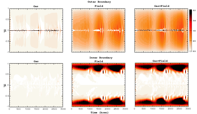
Figure 2: Plot of the latitude and time dependence of the gas and field components of $d{\dot{J}}/d\mu$ through the inner boundary ($r=R_{\ast}$; bottom panels) and the outer boundary ($r=15R_{\ast}$; top panels), for the standard model case. The colorbar is again normalized by the dipole-WD scaling of eqn. (20).

The colorscale in figure 2 illustrates this latitudinal distribution and time variation of the gas, magnetic and total (gas + magnetic) angular momentum loss $d{\dot{J}}/d\mu$ along both the inner and outer boundary for this standard model case. For the inner boundary, the broad white region at low latitudes emphasizes quite clearly now that the closed magnetic loops above the equatorial surface represent a kind of “dead zone” with little or no angular momentum loss. Instead, the mid-to-high latitudes of open field carry a strong concentration of the surface angular momentum loss. In contrast, at the outer boundary, there is a broad latitudinal distribution of angular momentum loss from the field, together with a equatorial concentration from the gas. Both the inner and outer boundary distribution of angular momentum also show a clear time variation associated with the ca. 1 Msec cycle of confinement, buildup, and release of material trapped in closed magnetic loops.

3.3.2 Time variability of latitudinally integrated ${\dot{J}}$

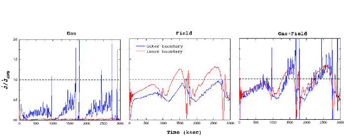
Figure 3: Time dependence of latitudinally integrated angular momentum loss ${\dot{J}}$ through both the inner and outer boundary, computed for the gas (left panel), field (middle) and the total for gas + field (right), in the standard model case.

The line plots in figure 3 compare the time dependence of the latitudinally integrated angular momentum loss, ${\dot{J}}$, for the gas, field, and total components, again evaluated at the inner (red curves) and the outer boundaries (blue curves). At the inner boundary, the gas component is negligible, with most of the angular momentum associated with the field. At the outer boundary, the gas component is highly variable, but still generally small compared to the field. The total angular momentum loss shows a nearly periodic variation, characterized by a gradual ramping up that ends in a sudden drop, with however a slight relative lag in the outer vs. inner variation. This lag reflects a cycle of storage and release of angular momentum within both the circumstellar field and gas.

The colorscale plots in figure 4 show also the full radius and time variation for the gas, magnetic, and total angular momentum loss, with the colorbar again normalized in units of the predicted dipole-WD scaling of eqn. (20). The results show quite vividly the intrinsic time variability, particularly for the gas component, which varies from intervals of little or no angular momentum loss, to a series of radially ejected streams, punctuated by a strong interval of loss during the magnetic breakout. The generally pale color reflects the fact that the overall level of gas angular momentum loss is a small fraction of the total expected from the dipole-WD scaling, particularly near the stellar surface. By comparison, the magnetic component is stronger and less variable. Overall, we see that the total angular momentum loss varies by about 50% above and below the predicted dipole-WD value from eqn. (20).

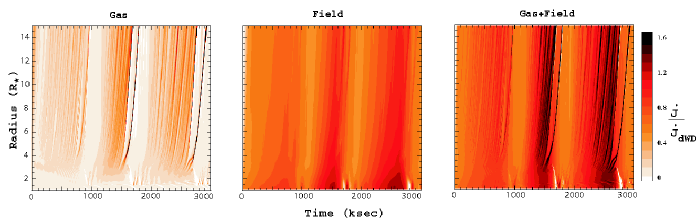
Figure 4: plots of the full radius and time variation of ${\dot{J}}$, again computed for gas, magnetic, and total components in the standard model, with the colorbar normalized in units of the predicted dipole-WD scaling of eqn. (20).

3.3.3 Spatial variation of time-averaged ${\dot{J}}$ for gas vs. magnetic component

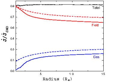
Figure 5: Radial variation of gas, field, and total angular momentum loss, again scaled by the total loss in the dipole-WD model. The solid curves show the time-averages from the standard numerical simulation model, while the dashed curves compare the corresponding WD scalings implied by eqn. (15), using the Alfvén radius $R_{A}$ from the dipole eqn. (19) assuming a $\beta=1$ velocity law and $\eta_{\ast}=100$.

To show more clearly the overall spatial variation, figure 5 plots the radial dependence of the time-averaged angular momentum loss for both the gas (blue curve) and magnetic field (red curve), along with the total loss (black curve). Note that this time-averaged total loss is nearly constant in radius, at a value that is remarkably close – about 90% – to the simple analytic dipole-WD predicted scaling!

Moreover, much as found in the WD67 monopole model, the angular momentum loss by the gas increases with radius, but still remains everywhere relatively small compared to the magnetic component. Indeed, the dashed curves compare the corresponding WD scalings given by eqn. (15), using the Alfvén radius $R_{A}$ from the dipole eqn. (19), and assuming a $\beta=1$ velocity law and $\eta_{\ast}=100$.

The good general agreement shows that, despite the complex time variation of the dipole case, the overall, time-averaged scaling of angular momentum loss can be quite well modeled through the simple monopole scalings of WD, as long as one just accounts for the different scaling of the Alfvén radius with the magnetic confinement parameter $\eta_{\ast}$.

3.4 Dependence on magnetic confinement and rotation parameters, $\eta_{\ast}$ and $W$

To build on this success in using the dipole WD scaling to characterize angular momentum loss in this standard case of moderately strong confinement and rotation, let us now examine how well this simple scaling agrees with the numerical simulation results for variations of magnetic confinement parameter $\eta_{\ast}$ and rotation parameter $W$.

Figure 6: Time-averaged angular momentum loss for all the models (triangles), plotted vs. $\eta_{\ast}$ (on a log-log scale), for both the $W=1/4$ (left) and $W=1/2$ rotation cases. The squares compare the scalings predicted by the dipole-WD approximation (20).

For the rotation cases $W=1/4$ and $W=1/2$, the lower and upper panels of figure 6 compare the variation of total, time-averaged angular momentum loss rate vs. $\eta_{\ast}$ (on a log-log scale) for both the numerical simulations (triangles) and analytic form (20) (squares). The overall agreement is remarkably good for both rotation cases, confirming that, quite independent of the rotation parameter $W$, this very simplified form (20) provides a good description of the scaling of the average angular momentum loss in this case of aligned dipoles.

Note that the ordinate axes in figure 6 are labeled in CGS units computed for the specific stellar model used in the simulations. But these specific values are essentially arbitrary. For any star of interest, the appropriate physical values can be readily derived from the dipole-WD scalings in eqn. (20). Indeed, the plot can likewise be characterized as giving the inverse of the spin-down time, which in the dipole-WD model has the specific scaling

$$\frac{\tau_{spin}}{\tau_{mass}}\approx\frac{\frac{3}{2}k}{\left[0.29+(\eta_{\ast}+0.25)^{1/4}\right]^{2}}\,.$$ (21)

Figure 7 shows the fraction of the gas and magnetic components of angular momentum loss at the outer boundary for each model, plotted vs. magnetic confinement parameter $\eta_{\ast}$ (again on a log scale), for both the $W=1/4$ (left) and $W=1/2$ (middle) rotation cases. For comparison, the right panel plots the corresponding large-radius scalings for the pure monopole model with a $\beta=1$ velocity law, as given by eqn. (17). For low and moderate magnetic confinement, $\eta_{\ast}\lesssim 30$, there is good general agreement between the analytic scalings and the numerical simulation results; but for stronger confinement, the numerical results show the gas fraction reaching a minimum and then increasing with increasing $\eta_{\ast}$.

The reasons for this increase are not entirely clear, but likely could be the result of the channeling and confinement of wind gas into the equatorial, nearly rigid-body disk discussed in paper 2. The magnetic torquing that spins this material up into a rigid disk represents a transfer of angular momentum from field to gas that has no parallel in the pure-outflow, monopole models of WD. Once sufficient material accumulates in this disk, the outward centrifugal force overwhelms the inward confinement of magnetic tension, leading to a breakout of this material that now carries outward a strong gas component of angular momentum loss.

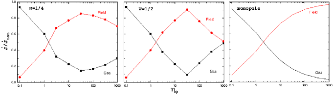
Figure 7: Fraction of the gas and magnetic components of angular momentum loss, plotted vs. magnetic confinement parameter $\eta_{\ast}$ (on a log scale), for both the $W=1/4$ (left) and $W=1/2$ (middle) rotation cases. The right panel shows analytic scalings for the pure monopole model with a $\beta=1$ velocity law, as given by eqn. (17).

4 Discussion

4.1 Role of mass-loss “Dead Zone”

A principal result of the above parameter study is that the overall level of angular momentum loss from an early-type star with a rotation-aligned dipole can be well described by the simple dipole-modified WD scaling given in eqn. (20). In this formulation, the mass loss rate and wind terminal speed used to compute the magnetic confinement parameter $\eta_{\ast}$ and associated spindown are those the star would have without a magnetic field, as set by the physics of radiative driving.

As shown in figure 8 of paper 2, the actual net mass loss rates in this parameter study of dipole winds show a significant decline with increasing confinement parameter $\eta_{\ast}$, fit roughly by the scaling relation [given in eqn. (24) of paper 2],

$$\frac{{\dot{M}_{\rm{B}}}}{{\dot{M}_{\rm{B}=0}}}\approx 1-\sqrt{1-R_{\ast}/R_{\rm{c}}}+1-\sqrt{1-0.5*R_{\ast}/R_{\rm{K}}}\,,$$ (22)

where $R_{\rm{c}}\approx R_{\ast}+0.7(R_{\rm{A}}-R_{\ast})$ is a maximum “closure” radius of magnetic loops, and $R_{\rm{K}}=R_{\ast}/W^{2/3}$ is the Kepler co-rotation radius. The former accounts for the effect of the mass loss “dead zone” of closed magnetic loops, while the latter corrects for the eventual centrifugal breakout that can occur from some initially closed loops above the Kepler radius.

In previous discussions of rotational spindown of magnetic winds, this dead zone has generally been presumed (e.g., Mestel, 1968a; Donati et al., 2006) to lead to a downward modification in the net angular momentum loss that would otherwise occur, based on the notion that the mass trapped in these closed loops does not (at least for loops closing below the Kepler radius) escape from the star, and thus should not contribute to the angular momentum loss.

This notion seems partly based on the perception that the gas itself is the principal direct carrier of the angular momentum loss. But both the WD67 analysis and the simulations here show that the dominant effect of the gas is indirect, inducing an azimuthal field component that then carries the bulk of the angular momentum loss, particularly near the stellar surface. Figure 2 shows that, even for this magnetic component, the closed loops at low latitudes do indeed represent a dead zone for loss of angular momentum, as well as mass. The net effect, however, seems merely to shunt a fixed total amount of angular momentum towards the mid-latitudes, carried by the azimuthal twisting of the open magnetic field. As the wind expansion opens up the field beyond the Alfvén radius, this transport of angular momentum spreads to cover all latitudes (cf. right vs. left panels of figure 2), and includes an increasing (but generally still minor) component for the gas (see figures 3, 4, 5, and 7).

So an important lesson of the above parameter study is that this additional dead-zone reduction in the net ${\dot{J}}$ does not apply to the dipole-modified WD scaling form (20). In a sense, it is already incorporated in the reduction associated with the change from the monopole scaling ${\dot{J}}\sim{\dot{M}}\eta_{\ast}$ to the dipole scaling ${\dot{J}}\sim{\dot{M}}\sqrt{\eta_{\ast}}$. To see this, note that, if we ignore the minor rotational correction of the Kepler term, the net mass loss reduction given by eqn. (22) has the strong-confinement ($\eta_{\ast}\gg 1$) scaling

$$\frac{{\dot{M}_{\rm{B}}}}{{\dot{M}_{\rm{B}=0}}}\approx 1-\left(1-\frac{R_{\ast}}{2R_{\rm{c}}}\right)\approx\frac{R_{\ast}}{1.4\,R_{\rm{A}}}~{}~{};~{}~{}R_{\rm{A}}\gg R_{\ast}\,.$$ (23)

If we now use this to apply a “dipole dead-zone” correction to the standard monopole scaling for angular momentum loss, we then find

$${\dot{J}}\sim{\dot{M}_{\rm{B}}}R_{A}^{2}\sim{\dot{M}_{\rm{B}=0}}R_{A}\sim{\dot{M}_{\rm{B}=0}}\sqrt{\eta_{\ast}}\,,$$ (24)

which thus reproduces the dipole scaling using the non-magnetic value for the mass loss rate!

The upshot then is that the dipole-modified scaling (20) using the non-magnetic mass loss rate effectively already accounts for the dead-zone reduction of the actual mass loss.

Table 1: Estimated Spindown Time for Selected Known Magnetic Stars.

Star	$M/M_{\odot}$	$R_{\ast}/R_{\odot}$	P (days)	k	${\dot{M}}\,(10^{-9}M_{\odot}/yr)$	$v_{\infty}~{}(1000~{}km/s)$	$B_{p}~{}(kG$)	$\eta_{\ast}$	$\tau_{spin}$(Myr)
$\theta^{1}$ Ori C 1	40	8	15.4	0.28	400	2.5	1.1	15.7	8
HD191612 2	40	18	538	0.17	6100	2.5	1.6	7.6	0.4
$\zeta$ Cas 3	8	5.9	5.37	0.1	0.3	0.8	0.34	3200	65.2
$\sigma$ Ori E 4	8.9	5.3	1.2	0.1	2.4	1.46	9.6	1.4 $\times 10^{5}$	1.4
$\rho$ Leo 5	22	35	7-47	0.12	630	1.1	0.24	20	1.1

4.2 Spindown time

From the above, the overall stellar spindown time is predicted to follow the scaling in eqn. (21). In the strong-confinement limit, this gives

$${\tau_{spin}} \approx {\tau_{mass}}\frac{\frac{3}{2}k}{\sqrt{\eta_{\ast}}}$$ (25)

$$\approx \frac{\frac{3}{2}kM}{B_{eq}R_{\ast}}\,\sqrt{\frac{v_{\infty}}{{\dot{M}}}}$$

$$\approx 1.1\times 10^{8}{\rm yr}~{}\frac{k}{B_{p}/kG}\,\frac{M/R_{\ast}}{M_{\odot}/R_{\odot}}\,\sqrt{\frac{V_{8}}{{\dot{M}}_{-9}}}\,.$$

Comparison with the monopole scaling (8) shows that the spindown is no longer independent of the mass loss rate, but now varies with its inverse square root. In addition, the dependencies on surface field and radius is now inverse linear instead of inverse square.

In practice, application of this scaling relation requires observational and/or theoretical inference of the various parameters. The last equality in (25) gives characteristic B2-star scalings for the mass loss, ${\dot{M}}_{-9}\equiv{\dot{M}}/(10^{-9}\,M_{\odot}$/yr), and wind speed, $v_{8}=v_{\infty}/(10^{8}\,$cm/s). Note that the magnetic field is now quoted as a surface value at the pole, $B_{p}$, and is scaled in kG. This is a typical value for known magnetic massive stars, as inferred from Stokes V measurement of photospheric lines with circular polarization by the Zeeman effect (see, e.g., Donati et al., 2002).

The mass to radius ratio $M/R_{\ast}$ can best be estimated from atmosphere models for the given spectral type, but generally for massive main sequence stars this should be just somewhat above the solar ratio. The moment of inertia constant $k$ can be estimated from stellar structure models, and should be typically $k\approx 0.1$, perhaps somewhat higher near the zero-age main sequence (ZAMS), and then decreasing by up to 50% with age (Claret, 2004).

Perhaps the most difficult parameters to infer are those for the stellar wind. Fortunately, these enter only in proportion to the square root of the ratio of wind speed to mass loss rate. But because the actual values for both of these are likely to be strongly affected by the magnetic field, it may generally be better not to infer them from direct observations for the actual star in question, but rather to use the inferred spectral type to apply observational or theoretical scaling laws for the values in similar non-magnetic stars.

Table 1 lists spindown times based on estimated parameters for a sample of known magnetic hot stars. The first two known magnetic O-stars, $\theta^{1}$ Ori C (Donati et al., 2002) and HD 191612 (Donati et al., 2006), are both slow rotators, with periods of respectively 15 d and 538 d. $\theta^{1}$ Ori C is thought to be quite young, less than 0.2 Myr, and so still on the ZAMS, while HD 191612 is thought to be more evolved, with an age of 2-3 Myr. Using parameters quoted in Donati et al. 2006, we infer corresponding spindown times of respectively $\sim$8 Myr and $\sim$0.4 Myr. This implies that magnetic wind braking seems unlikely to explain the slow rotation of $\theta^{1}$ Ori C, but it does seem potentially relevant for HD 191612. Alternatively, magnetic effects during star formation could have lead to an initial slow rotation.

For He-strong stars, a key object is the B2V star $\sigma$ Ori E. This has an estimated polar field strength of $B_{kG}\approx 9.6$, and with remaining parameters as in table 1, we estimate a spindown time of $\sim$1.4 Myr. As a main sequence B2 star, its age is likely comparable to this. The rotation period, 1.2 d, is still quite short, about twice that for critical rotation, implying only a moderate net spindown since formation.

4.3 Extension to non-aligned dipoles and higher multipoles

However note that, as is typical of magnetic massive stars, most of the above cases exhibit dipole fields with a significant tilt angle to the rotation axis. MHD simulation of such a tilted dipole requires accounting for 3-D, non-axisymmetric outflow as the polar field sweeps around in azimuth. This remains a challenge for future studies. Without such simulations, we can only offer some general speculations on how such a tilt might affect the spindown. Generally, it seems that angular momentum loss should be modestly enhanced, because of the factor two stronger polar field.

But another factor might be the open nature of this polar field. One might expect this to lead to a larger magnetic moment arm, perhaps even following the stronger monopole scaling, ${\dot{J}}\sim\eta_{\ast}$, rather than the dipole form ${\dot{J}}\sim\sqrt{\eta_{\ast}}$. But the analysis in the Appendix suggests that such magnetic polar-axis fields in an oblique rotation case should actually follow a weaker spindown scaling, ${\dot{J}}\sim\eta_{\ast}^{1/3}$. This implies that, much as in the aligned-dipole case, the overall, spherically averaged loss rate for an oblique-dipole wind should still be dominated by the regions surrounding closed loops, with a net scaling that thus is similar to the aligned case.

In some magnetic hot stars, the inferred field is manifestly non-dipole. For example, the B2IVp He-strong star HD 37776 (V901 Ori) has been inferred to have quadrupole field that dominates any dipole component, with peak strength of $\sim$10 kG (Thompson & Landstreet, 1985). The luminosity class IV would normally imply an evolved, main-sequence star, but the still moderately short rotation period of 1.5387 d seems to suggest little spindown. If we assume a somewhat larger radius and higher mass loss rate than $\sigma$ Ori E, so that the non-magnetic parameters in (25) may be near unity, then applying the inferred field of 10 kG gives a spindown time of $\sim$1.1 Myr.

Moreover, although detailed predictions must await 3-D MHD simulations of such a quadrupole (or higher multipole) case, one might infer that the steeper radial decline of the quadrupole field should lead to a weaker spindown. For a general field scaling with $r^{-q}$, with $q=3$ for a dipole and $q=4$ for a quadrupole, the ratio of magnetic to wind energy should decline as $r^{2-2q}$, implying an Alfvén radius that scales as $R_{A}\sim\eta_{\ast}^{1/(2q-2)}$, or $R_{A}\sim\eta_{\ast}^{1/6}$ for a quadrupole. In the strong-confinement limit, the expected spindown scaling should thus become

$$\frac{\tau_{spin,quad}}{\tau_{mass}}\approx\frac{\frac{3}{2}k}{\eta_{\ast}^{1/3}}\,.$$ (26)

Compared to a dipole of the same surface strength, the spindown time for a quadrupole would thus be about a factor $\eta_{\ast}^{1/6}$ longer. This might seem like a weak correction, but for He-strong stars of spectral type B2, the low mass loss means that a surface field of 10 kG gives a confinement parameter of $\eta_{\ast}\approx 10^{7}$, thus implying a factor $\sim$10 times longer spindown for a quadrupole vs. a dipole of same surface strength. In this context, the expected spindown time for HD 37776 becomes of order $\sim$10 Myr.

On the other hand, the presence of a more complex field might make it easier for the wind to break open the magnetic flux associated with large-scale dipole component, and so allow a more extended magnetic moment arm. In principal, this could even lead to a stronger spindown effect. Mikulášek & et al. (2008) have recently reported a direct measurement of rotational spindown in HD 37776. They infer a $17.7\pm 0.7$ second increase in the 1.5387 day period over a span of 31 years, translating to a spindown time of just 0.23 Myr! This is substantially shorter than the above dipole estimate from wind torquing. Indeed, the luminosity class IV would normally imply an evolved, main-sequence star, but the still moderately rapid rotation together with the very rapid spindown seem to require a very young age.

Overall, the study of angular momentum loss in these more non-aligned dipole or higher-order multipole cases must await further, 3-D MHD simulation studies.

4.4 No sudden spindown during breakout events

In a few magnetic stars, there appears to be evidence for sudden change in rotation period. For the rapidly rotating Ap star CU Virginis (HD 124224), Trigilio et al. (2008) cite radio observations indicating changes in rotational phase over 20 years, identified with two discrete period increases of 2.18 s in 1984 and about 1 s in 1999. In terms of the still-rapid rotation period 0.52 days, the associated average spindown timescale over this 15 year timespan is quite short, only about 300,000 years. These sudden period changes could be associated with changes in the star’s internal structure (Stȩpień, 1998); but Trigilio et al. (2008) suggest they might also be the result of a sudden emptying of mass accumulated in the star’s magnetosphere.

The simulations here do indeed show repeated episodes of substantial emptying, but careful examination indicates that these do not lead to sudden jumps in the angular momentum of the star itself. Both figures 2 and 3 show, for example, that angular momentum loss through the stellar surface varies smoothly through the cycle of magnetosphere build-up and release, and if anything is actually less during the sudden breakouts that characterize magnetospheric emptying. In terms of stellar rotation, the outward transfer of angular momentum to the magnetosphere occurs gradually, as the magnetosphere fills up, effectively increasing the moment of inertia of the star+magnetosphere system. As such, when the emptying does occur, it merely represents the final escape for angular momentum that had already been lost to the star. Moreover, most of the angular momentum is not even contained in the trapped gas, but rather in the stressed magnetic field, which figure 3b shows varies quite smoothly from the stellar surface.

Thus, even apart from questions of the magnitude of angular momentum loss needed to explain the average spindown inferred for CU Vir, magnetospheric emptying does not seem well-suited to explaining the claimed suddenness of rotation changes in this star.

4.5 Comparison with previous spindown analyses

Past studies of wind magnetic spindown have primarily focussed on cool, low-mass, solar-type stars. The main analysis aimed specifically at spindown for hotter, higher-mass star, the main analysis was by FM84, who derived 1-D, steady-state solutions for the equatorial flow of a CAK-type line-driven wind from a rotating hot star with a Weber-Davis style monopole magnetic field. To ensure their steady solutions passed smoothly through the various flow critical points (i.e., those associated with Alfvén, slow-mode, and fast-mode MHD waves, as well as the usual CAK critical point), they had to use a quite elaborate numerical iteration scheme; as such, they do not quote any simple scaling forms for the Alfvén radius and associated spindown rate.

Instead, their Table 1 lists numerical results for a set of 16 models with various rotation rates and field strengths, assuming fixed stellar and wind parameters for a typical O-supergiant. We find here that these results can be generally well fit (within ca. 10-15%) by the simple general monopole scaling for $R_{A}$, eqn. (5).

However, FM84 quote spindown times as low as 60,000 years, i.e., for their case 4, with field strength of 1600 G, and mass loss rate of $5.32\times 10^{-6}M_{\odot}/{\rm yr}$. The associated confinement parameter is $\eta_{\ast}\approx 80$. Since the angular momentum loss rate for an aligned dipole is a factor $\sqrt{\eta_{\ast}}$ lower than for a monopole, we see that a dipole with a similar surface field strength (1600 G) as FM84 model 4 would have about a factor 9 longer spindown time, or now about 0.5 Myr. In contrast, their weaker-field model, e.g. case 1 with only 200 G, has a confinement parameter $\eta_{\ast}\approx 1.7$, implying only about a 30% dipole increase above the 2 Myr spindown time quoted for this case by the FM84 monopole analysis. Overall, the dipole modifications in spindown rate found here suggest that the upper limits on surfaced field strength inferred by MacGregor et al. (1992) for rotating hot-stars are likely to be too low.

For cooler, solar-type stars with coronal-type pressure-driven winds, the literature on wind magnetic spindown is more extensive, and includes both semi-analytic studies (Okamoto, 1974; Mestel, 1984; Tout & Pringle, 1992) and numerical iterations or simulations, (Sakurai, 1985; Washimi & Shibata, 1993; Keppens & Goedbloed, 2000; Matt & Balick, 2004). In addition to spindown by a magnetized coronal wind during the star’s main sequence phase, there has been extensive study of angular momentum loss during pre-main-sequence accretion through a magnetized disk during a T-Tauri star (TTS) phase. Most recently, Matt & Pudritz (2008) report on 2-D MHD simulations of spindown by an aligned dipole field in a coronal wind during the TTS phase. With some translation for differences in notation and parameter definition, many of their results seem quite analogous to those reported here for hot-star winds. In particular, their eqn. (14) for the Alfvén radius is quite similar to the dipole scaling in eqn. (19) here, just replacing $v_{\infty}$ with the (numerically comparable) surface escape speed $v_{esc}$, with their numerical best-fit exponent $m=0.223$ very similar to our $1/4=0.25$.

5 Summary and Future Outlook

This paper analyzes the nature of angular momentum loss by radiatively driven winds from hot-stars with a dipole magnetic field aligned to the stellar rotation axis. It applies our previous MHD simulation study from paper 2, which consisted of a 2-parameter series of models, dependent on the critical rotation ratio $W$, and on the magnetic confinement parameter $\eta_{\ast}$. Key results can be summarized as follows:

• As shown in figure 6, for both slow ($W=1/4$) and moderate rotation ($W=1/2$), the time-averaged, total angular momentum loss rate, ${\dot{J}}$, follows closely a dipole-modified version of the Weber-Davis scaling of eqn. (1).

• Specifically, in the dipole case, the Alfvén radius has a weaker dependence on magnetic confinement parameter, with a strong confinement scaling as $R_{A}\sim\eta_{\ast}^{1/4}$ vs. as $R_{A}\sim\sqrt{\eta_{\ast}}$ for the monopole [cf. eqns. (19) and (5)].

• This leads to a dipole scaling for ${\dot{J}}$, given by eqn. (20), that is weaker than for a monopole, by a factor $1/\sqrt{\eta_{\ast}}$ in the strong-confinement limit. It also implies a correspondingly longer spindown time.

• As in the WD67 monopole case, the total angular momentum loss is generally dominated by the magnetic component. However, in the strongest confinement models, there is trend toward increasing contribution by the gas, apparently a consequence of the eventual breakout of equatorially trapped material.

• The dipole nature of the field gives the angular momentum transport a complex variation in radius, latitude, and time, consisting of long intervals of gradual build-up, punctuated by episodic breakouts of material trapped in an equatorial disk.

• However, the gradual buildup and storage of angular momentum in the circumstellar field and gas implies that the stellar spindown rate is likewise gradual, with no sudden jumps during intervals of breakout. As such, “magnetospheric emptying” does not seem like a likely explanation for sudden jumps in rotation rate claimed in some magnetic hot-stars.

• The “dead zone” of closed loops surrounding the equator does inhibit the equatorial loss of angular momentum from the near the stellar surface, but the net effect is merely to shunt the angular momentum flux to a magnetic component at mid-latitudes. The upshot is that the overall dipole scaling for total ${\dot{J}}$ effectively already accounts for any dead-zone reduction.

The 2-D, time-dependent models here for rotation-aligned dipole thus provide a much richer physical picture for angular momentum loss than inferred in the 1-D, steady models for the WD67 idealization of a monopole field. However, proper interpretation for the broad population of hot-stars inferred to have tilted dipoles or even multipole fields will require even more challenging 3-D MHD simulation models that explicitly allow for variations in azimuth as well as latitude and radius. Developing such fully 3-D MHD simulations for these cases is thus a major focus of our planned future research.

Appendix A Angular momentum flux from magnetic pole for oblique rotator

To gain insight into the relative effectiveness of angular momentum loss for the case of non-aligned dipole, let us extend the WD67 monopole analysis to the 1-D flow directly along the magnetic pole of an oblique dipole, i.e., with axis now perpendicular to the rotation. This flow tube has a radial orientation, but its areal expansion is some factor $h(r)$ faster than $r^{2}$, so that both radial mass flux and radial field strength now vary as $\rho v_{r}\sim B_{r}\sim 1/hr^{2}$. Following eqn. (20) of Owocki & ud-Doula (2004), we can approximate this expansion factor by

$$h(r)=\frac{r}{R_{\ast}}\,\frac{R_{\ast}+R_{A}}{r+R_{A}}\,,$$ (27)

where we take their “confinement radius” $R_{c}=R_{A}$.

The analysis then proceeds analogously to the WD monopole case summarized in section 2.3, leading again to an equation of the form (14), except that now the quantities ${\dot{m}}\equiv 4\pi\rho vr^{2}$, and thus $j_{eq}\equiv{\dot{J}}_{eq}/{\dot{m}}$, are no longer constant in radius. Instead, in terms of the constant mass loss rate ${\dot{M}}$, we have ${\dot{m}}(r)={\dot{M}}/h(r)$. Continuity at the Alfvén critical point again requires $j_{eq}=\Omega R_{A}^{2}$, but this now implies an angular momentum loss that scales as

$${\dot{J}}_{eq}={\dot{M}}\frac{\Omega R_{A}^{2}}{h_{A}}\,,$$ (28)

where $h_{A}\equiv h(R_{A})=(1+R_{A}/R_{\ast})/2$.

Since $\rho v_{r}\sim B_{r}\sim 1/hr^{2}$ along this dipole-axis flow, the ratio of magnetic to flow energy follows the scaling

$$\eta(r)\equiv\frac{B^{2}}{4\pi\rho v_{r}^{2}}=\frac{4\eta_{\ast}R_{\ast}^{2}}{h(r)r^{2}(1-R_{\ast}/r)^{\beta}}\,,$$ (29)

where the factor 4 accounts for the fact that $\eta_{\ast}$ is defined in terms of $B_{eq}^{2}=B_{p}^{2}/4$. Ignoring for simplicity the radial variation of velocity (effectively using $\beta=0$), the Alfvén condition $\eta(R_{A})\equiv 1$ thus implies $(R_{A}/R_{\ast})^{2}=4\eta_{\ast}/h_{A}$, and so

$${\dot{J}}_{eq}={\dot{M}}\,\Omega R_{\ast}^{2}\frac{4\eta_{\ast}}{h_{A}^{2}}={\dot{M}}\,\Omega R_{\ast}^{2}\frac{16\eta_{\ast}}{\left(1+R_{A}/R_{\ast}\right)^{2}}\,.$$ (30)

In the strong confinement limit $\eta_{\ast}\gg 1$, we find $R_{A}/R_{\ast}\approx 2\eta_{\ast}^{1/3}$, which gives

$${\dot{J}}_{eq}\approx{\dot{M}}\,\Omega R_{\ast}^{2}~{}4\eta_{\ast}^{1/3}~{}~{};~{}~{}\eta_{\ast}\gg 1\,.$$ (31)

Comparing this to the monopole scaling ${\dot{J}}\sim\eta_{\ast}$ and the aligned-dipole scaling ${\dot{J}}\sim\sqrt{\eta_{\ast}}$, we see that this oblique dipole-axis has an angular momentum loss rate that is weaker than either of them, scaling only as ${\dot{J}}\sim\eta_{\ast}^{1/3}$.

References

- Castor et al. (1975) Castor J. I., Abbott D. C., Klein R. I., 1975, ApJ, 195, 157
- Claret (2004) Claret A., 2004, A&A, 424, 919
- Donati et al. (2002) Donati J.-F., Babel J., Harries T. J., Howarth I. D., Petit P., Semel M., 2002, MNRAS, 333, 55
- Donati et al. (2006) Donati J.-F., Howarth I. D., Bouret J.-C., Petit P., Catala C., Landstreet J., 2006, MNRAS, 365, L6
- Friend & MacGregor (1984) Friend D. B., MacGregor K. B., 1984, ApJ, 282, 591
- Groote & Hunger (1982) Groote D., Hunger K., 1982, A&A, 116, 64
- Kawaler (1988) Kawaler S. D., 1988, ApJ, 333, 236
- Keppens & Goedbloed (2000) Keppens R., Goedbloed J. P., 2000, ApJ, 530, 1036
- Kholtygin et al. (2007) Kholtygin A. F., Fabrika S. N., Burlakova T. E., Valyavin G. G., Chuntonov G. A., Kudryavtsev D. O., Kang D., Yushkin M. V., Galazutdinov G. A., 2007, Astronomy Reports, 51, 920
- Krtička et al. (2006) Krtička J., Kubát J., Groote D., 2006, A&A, 460, 145
- MacGregor & Cassinelli (2003) MacGregor K. B., Cassinelli J. P., 2003, ApJ, 586, 480
- MacGregor & Charbonneau (1999) MacGregor K. B., Charbonneau P., 1999, ApJ, 519, 911
- MacGregor et al. (1992) MacGregor K. B., Friend D. B., Gilliland R. L., 1992, A&A, 256, 141
- Matt & Balick (2004) Matt S., Balick B., 2004, ApJ, 615, 921
- Matt & Pudritz (2008) Matt S., Pudritz R. E., 2008, ApJ, 678, 1109
- Mestel (1968a) Mestel L., 1968a, MNRAS, 138, 359
- Mestel (1968b) Mestel L., 1968b, MNRAS, 140, 177
- Mestel (1984) Mestel L., 1984, in Baliunas S. L., Hartmann L., eds, Cool Stars, Stellar Systems, and the Sun Vol. 193 of Lecture Notes in Physics, Berlin Springer Verlag, Angular Momentum Loss During Pre-Main Sequence Contraction. pp 49–+
- Mestel & Spruit (1987) Mestel L., Spruit H. C., 1987, MNRAS, 226, 57
- Mikulášek & et al. (2008) Mikulášek Z., et al. 2008, A&A, 485, 585
- Mullan & MacDonald (2001) Mullan D. J., MacDonald J., 2001, ApJ, 559, 353
- Mullan & MacDonald (2005) Mullan D. J., MacDonald J., 2005, MNRAS, 356, 1139
- Neiner et al. (2003) Neiner C., Geers V. C., Henrichs H. F., Floquet M., Frémat Y., Hubert A.-M., Preuss O., Wiersema K., 2003, A&A, 406, 1019
- Okamoto (1974) Okamoto I., 1974, MNRAS, 166, 683
- Owocki & ud-Doula (2004) Owocki S. P., ud-Doula A., 2004, ApJ, 600, 1004
- Sakurai (1985) Sakurai T., 1985, A&A, 152, 121
- Smith & Bohlender (2007) Smith M. A., Bohlender D. A., 2007, A&A, 466, 675
- Stȩpień (1998) Stȩpień K., 1998, A&A, 337, 754
- Stone & Norman (1992) Stone J. M., Norman M. L., 1992, ApJS, 80, 753
- Suess & Nerney (1975) Suess S. T., Nerney S. F., 1975, Sol. Phys., 40, 487
- Thompson & Landstreet (1985) Thompson I. B., Landstreet J. D., 1985, ApJ, 289, L9
- Tout & Pringle (1992) Tout C. A., Pringle J. E., 1992, MNRAS, 256, 269
- Trigilio et al. (2008) Trigilio C., Leto P., Umana G., Buemi C. S., Leone F., 2008, MNRAS, 384, 1437
- ud-Doula & Owocki (2002) ud-Doula A., Owocki S. P., 2002, ApJ, 576, 413
- ud-Doula et al. (2008) ud-Doula A., Owocki S. P., Townsend R. H. D., 2008, MNRAS, 385, 97
- Washimi & Shibata (1993) Washimi H., Shibata S., 1993, MNRAS, 262, 936
- Weber & Davis (1967) Weber E. J., Davis L. J., 1967, ApJ, 148, 217