Comparing iterative methods to compute the overlap Dirac operator at nonzero chemical potential

Abstract:

The overlap Dirac operator at nonzero quark chemical potential involves the computation of the sign function of a non-Hermitian matrix. In this talk we present iterative Krylov subspace approximations, with deflation of critical eigenvalues, which we developed to compute the operator on large lattices. We compare the accuracy and efficiency of two alternative approximations based on the Arnoldi and on the two-sided Lanczos method. The short recurrences used in the latter method make it faster and more effective for realistic lattice simulations.

1 The overlap Dirac operator at nonzero chemical potential

Although chiral symmetry can not be implemented exactly in a space-time discretization of QCD [1], a lattice version of chiral symmetry can be obtained by a renormalization group blocking transformation. The ensuing lattice chiral symmetry is embodied by the Ginsparg-Wilson relation [2], which is solved by the overlap Dirac operator proposed by Narayanan and Neuberger [3, 4].

Astrophysical objects like neutron stars exhibit an abundance of quarks over anti-quarks, and the study of QCD in such a background necessitates the introduction of a quark chemical potential $\mu$ in the QCD Lagrangian. In this situation chiral symmetry still holds and in Ref. [5] two of the present authors proposed an extension of the overlap Dirac operator to nonzero chemical potential which still satisfies the Ginsparg-Wilson relation,

$$D_{\text{ov}}(\mu)=\mathbbm{1}+\gamma_{5}\operatorname{sgn}(\gamma_{5}D_{\text{w}}(\mu))\>,$$ (1)

where $\gamma_{5}=\gamma_{1}\gamma_{2}\gamma_{3}\gamma_{4}$ with $\gamma_{1},\ldots,\gamma_{4}$ the Dirac gamma matrices in Euclidean space, $\operatorname{sgn}$ is the matrix sign function, and

$$D_{\text{w}}(\mu)=\mathbbm{1}-\kappa\sum_{i=1}^{3}(T_{i}^{+}+T_{i}^{-})-\kappa({e^{\mu}}T_{4}^{+}+{e^{-\mu}}T_{4}^{-})$$ (2)

is the Wilson Dirac operator at nonzero chemical potential [6] with $(T^{\pm}_{\nu})_{yx}=(\mathbbm{1}\pm\gamma_{\nu})U_{x,\pm\nu}\delta_{y,x\pm\hat{\nu}}$, $\kappa=1/(8+2m_{\text{w}})$, $m_{\text{w}}\in(-2,0)$ and $U_{x,\pm\nu}\in$ SU(3). The exponential factors $e^{\pm\mu}$ implement the quark chemical potential on the lattice.

For $\mu\neq 0$ the argument $\gamma_{5}D_{\text{w}}(\mu)$ of the sign function becomes non-Hermitian, and one is faced with the problem of defining and computing the sign function of a non-Hermitian matrix. If the matrix $A$ of dimension $N$ is diagonalizable, then $A=U\operatorname{diag}\{\lambda_{i}\}U^{-1}$ with eigenvalues $\lambda_{i}$ and eigenvector matrix $U$, and a function $f(A)$ can be computed using the spectral definition [7]

$$f(A)=U\operatorname{diag}\{f(\lambda_{i})\}U^{-1}\>.$$ (3)

If $A$ is not diagonalizable one can still apply an extension of the spectral definition using the Jordan canonical form. As the eigenvalues of a general matrix $A$ can be complex, the sign function computed using Eq. (3) requires the sign of a complex number, which can be defined by

$$\operatorname{sgn}(z)\equiv\frac{z}{\sqrt{z^{2}}}=\operatorname{sgn}(\operatorname{Re}z)\>,$$ (4)

where the branch cut of the square root is chosen along the negative real axis. This definition ensures that $(\operatorname{sgn}z)^{2}=1$ and gives the usual result when $z$ is real. It is straightforward to check that this definition ensures that $(\operatorname{sgn}A)^{2}=\mathbbm{1}$. Therefore the overlap Dirac operator at $\mu\neq 0$ satisfies the Ginsparg-Wilson relation, and the operator can have exact zero modes with definite chirality. The main properties of the operator were discussed in Ref. [8].

Since its introduction the operator has been validated in a number of studies: Its definition is consistent with that of domain wall fermions at $\mu\neq 0$ when the extension of the fifth dimension is taken to infinity and its lattice spacing taken to zero [8], its microscopic density and first peak computed from quenched lattice simulations on a $4^{4}$ lattice agree with the predictions of non-Hermitian chiral random matrix theory [5, 9], and the free fermion energy density was shown to have the correct continuum limit [10, 11].

2 Arnoldi approximation for a function of a non-Hermitian matrix

The exact computation of $\operatorname{sgn}(A)$ using the spectral definition (3) is only feasible for small lattice volumes as the memory requirements to store the full matrix and the computation time needed to perform a full diagonalization become prohibitively large for realistic lattice volumes. Therefore it is necessary to develop iterative Krylov subspace methods to compute $f(A)b$ for vectors $b$. For Hermitian matrices the corresponding methods have already reached a high level of sophistication and are widely applied, but for non-Hermitian matrices such methods are novel, except for the special cases of the inverse and the exponential function. The Arnoldi approximation discussed below was first introduced in Ref. [12], while the two-sided Lanczos approximation of Sec. 4 was presented in Ref. [13].

Such iterative methods are based on the observation that the unique polynomial $P_{K}(z)$ of order $K\leq N-1$ which interpolates $f(z)$ at all the eigenvalues of $A$ satisfies the equality

$$P_{K}(A)b=f(A)b\quad\text{ for {any} vector $b$}\>,$$ (5)

as follows from the definition (3). Therefore it is an obvious endeavor to construct a good low-degree polynomial approximation for $y=f(A)b$, taking into account the spectrum of $A$ and the decomposition of $b$ in the eigenvectors of $A$.

In order to construct such a low order polynomial approximation to $f(A)b$ we consider the Krylov subspace $K_{k}(A,b)=\operatorname{span}(b,Ab,A^{2}b,\ldots,A^{k-1}b)$. By definition this subspace contains all the vectors resulting from the action of an arbitrary polynomial of degree $\leq k-1$ in $A$ on the source vector $b$. One of these vectors, namely the orthogonal projection of $f(A)b$ on the Krylov subspace, will minimize $||P_{k-1}(A)b-f(A)b||$ over all polynomials of degree $\leq k-1$.

The Arnoldi method uses the recursive scheme

$$AV_{k}=V_{k}H_{k}+\beta_{k}v_{k+1}e_{k}^{T}$$ (6)

with

$$V_{k}^{\dagger}AV_{k}=H_{k}$$ (7)

to build an orthonormal basis $V_{k}=(v_{1},\ldots,v_{k})$ in $K_{k}(A,b)$, where $v_{1}=b/|b|$, $\beta_{k}$ is the normalization of $v_{k+1}$, and $e_{k}$ is the $k$-th basis vector in $\mathbb{C}^{k}$. The matrix $H_{k}$ is a Hessenberg matrix (upper triangular + one subdiagonal) of dimension $k$, whose eigenvalues are called the Ritz values of $A$ w.r.t. $K_{k}(A,b)$.

Once the Arnoldi basis has been constructed, the projection of $y=f(A)b$ on $K_{k}(A,b)$ can be written as

$$y_{\text{proj}}=V_{k}V_{k}^{\dagger}f(A)b=V_{k}V_{k}^{\dagger}f(A)V_{k}V_{k}^{\dagger}b\>.$$ (8)

This formal expression requires the knowledge of the exact solution and is therefore of no practical use. However, using the Ritz approximation

$$V_{k}^{\dagger}f(A)V_{k}\approx f(H_{k})\>,$$ (9)

which is based on Eq. (7), allows us to approximate the projection by

$$y_{\text{proj}}\approx\tilde{y}=|b|V_{k}f(H_{k})e_{1}\>.$$ (10)

By construction this approximation is an element of the Krylov subspace $K_{k}(A,b)$, and it can be shown that the implicit polynomial constructed by this approximation interpolates $f(x)$ at the Ritz values of $A$ w.r.t. $K_{k}(A,b)$ [14]. Note that only the first column of $f(H_{k})$ is needed in Eq. (10).

This approximation reduces the problem to the computation of $f(H_{k})$ with $\dim H_{k}\ll\dim A$, which makes it very useful for practical use. The inner sign function $f(H_{k})$ will then be computed with one’s method of choice. This could be an exact spectral decomposition if $k$ is small, or some suitable approximation method, e.g., Roberts’ matrix-iterative method for the sign function,

$$S^{n+1}=\frac{1}{2}\left[S^{n}+(S^{n})^{-1}\right]\qquad\text{with}\quad S^{0}=H_{k}\>,$$

which converges quadratically to $\operatorname{sgn}(H_{k})$.

3 Sign function and deflation

When computing the sign function of the matrix $A$ an additional problem occurs when the matrix has small eigenvalues, as large Krylov subspaces are then required to achieve a good accuracy. The reason is that it is not possible to approximate $f$ well by a low-degree polynomial over the entire spectrum of $A$ if it varies too rapidly in a small subregion. A solution to this problem is to use the exact value of $f$ for a number of critical eigenvalues of $A$. Over the remaining part of the spectrum $f$ should then behave well enough to allow for a low-degree polynomial approximation.

Implementing this so-called deflation is straightforward in the Hermitian case, where it is based on the fact that any number of eigenvectors span a subspace orthogonal to the remaining eigenvectors. In the non-Hermitian case the eigenvectors of $A$ are no longer orthogonal, and a more involved approach is needed. We have previously proposed two alternative deflation variants for this case [12]. Herein we only present the left-right (LR) deflation and refer to Ref. [12] for the details of the Schur deflation.

The method needs the left and right eigenvectors belonging to the $m$ critical eigenvectors,

$$AR_{m} =R_{m}\Lambda_{m}\>,\qquad L_{m}^{\dagger}A=\Lambda_{m}L_{m}^{\dagger}\>,$$ (11)

where $\Lambda_{m}$ is the diagonal eigenvalue matrix for the $m$ critical eigenvalues and $R_{m}=(r_{1},\ldots,r_{m})$ and $L_{m}=(\ell_{1},\ldots,\ell_{m})$ are the matrices of right and left eigenvectors, respectively. These matrices can be made bi-orthonormal, i.e., $L_{m}^{\dagger}R_{m}=I_{m}$, such that $R_{m}L_{m}^{\dagger}$ is an oblique projector on the subspace $\Omega_{m}$ spanned by the right eigenvectors.

If the source vector is decomposed as

$$b=b_{\parallel}+b_{\ominus}\>,$$ (12)

where $b_{\parallel}=R_{m}L_{m}^{\dagger}b$ is an oblique projection of $b$ on $\Omega_{m}$ and $b_{\ominus}=b-b_{\parallel}$, then the matrix function can be written as

$$f(A)b=\underbrace{f(A)R_{m}L_{m}^{\dagger}b}_{\text{exact}}\>\>\>\>+\underbrace{f(A)b_{\ominus}}_{\text{approximation}}\>.$$ (13)

The contribution of the first term can be computed exactly, while the second term can be approximated by the Arnoldi method described in Sec. 2 applied to the Krylov subspace $K_{k}(A,b_{\ominus})$. The final approximation is then given by

$$f(A)b\approx R_{m}f(\Lambda_{m})L_{m}^{\dagger}b+|b_{\ominus}|V_{k}f(H_{k})e_{1}\>.$$ (14)

As before the function $f(H_{k})$ of the internal matrix should be computed with a suitable method. The critical eigenvalues with their left and right eigenvectors should be computed once for all source vectors $b$.

4 Two-sided Lanczos approximation

The Arnoldi method described in Sec. 2 suffers from the long recurrences used to orthogonalize the Arnoldi basis. As an alternative we now consider the two-sided Lanczos method which uses short recurrences at the cost of giving up orthogonality for bi-orthogonality.

Consider the two Krylov subspaces $K_{k}(A,b)$ and $K_{k}(A^{\dagger},b)$ and construct two bi-orthogonal bases $V_{k}$ and $W_{k}$ such that $W_{k}^{\dagger}V_{k}=I_{k}$ and the matrix $G_{k}\equiv W_{k}^{\dagger}AV_{k}$ is tridiagonal with

$$G_{k}\equiv W_{k}^{\dagger}AV_{k}=\begin{pmatrix}\alpha_{1}&\gamma_{1}&0&\cdots&0\\ \beta_{1}&\alpha_{2}&\ddots&\ddots&\vdots\\ 0&\ddots&\ddots&\ddots&0\\ \vdots&\ddots&\ddots&\ddots&\gamma_{k-1}\\ 0&\cdots&0&\beta_{k-1}&\alpha_{k}\\ \end{pmatrix}.$$ (15)

It can be shown that $V_{k}$ and $W_{k}$ can be built using the short recurrence relations

$$\left\{\begin{aligned} \beta_{i}v_{i+1}&=(A-\alpha_{i})v_{i}-\gamma_{i-1}v_{i-1}\>,\\ \gamma_{i}^{*}w_{i+1}&=(A^{\dagger}-\alpha_{i}^{*})w_{i}-\beta_{i-1}^{*}w_{i-1}\>,\end{aligned}\right.$$ (16)

where $v_{1}=w_{1}=b/|b|$, $\alpha_{i}=w_{i}^{\dagger}Av_{i}$, and $\beta_{i}$ and $\gamma_{i}$ are determined from the normalization condition $w_{i+1}^{\dagger}v_{i+1}=1$.

The matrix $V_{k}W_{k}^{\dagger}$ is an oblique projector on $K_{k}(A,b)$, such that an oblique projection of $f(A)b$ on $K_{k}(A,b)$ is obtained using

$$y\approx y_{\text{obl}}=V_{k}W_{k}^{\dagger}f(A)V_{k}W_{k}^{\dagger}b\>.$$ (17)

In analogy to the Arnoldi method we introduce the approximation $W_{k}^{\dagger}f(A)V_{k}\approx f(G_{k})$ such that

$$y_{\text{obl}}\approx\tilde{y}=|b|V_{k}f(G_{k})e_{1}\>.$$ (18)

The approximation $\tilde{y}\in K_{k}(A,b)$, and the problem is now reduced to the computation of $f(G_{k})$ with $\dim G_{k}\ll\dim A$.

If the matrix $A$ has small eigenvalues, deflation will again be necessary when computing the sign function. To implement the LR-deflation in this case one constructs two bi-orthogonal bases $V_{k}$ and $W_{k}$ in $K_{k}(A,b_{\ominus}^{R})$ and $K_{k}(A^{\dagger},b_{\ominus}^{L})$, where the directions along $R_{m}$, respectively $L_{m}$, have been fully deflated from $b$, i.e., $b_{\ominus}^{R}=(1-R_{m}L_{m}^{\dagger})b$ and $b_{\ominus}^{L}=(1-L_{m}R_{m}^{\dagger})b$. With LR-deflation the function approximation becomes

$$f(A)b\approx R_{m}f(\Lambda_{m})L_{m}^{\dagger}b+|b_{\ominus}^{R}|V_{k}f(G_{k})e_{1}\>.$$ (19)

5 Results

In this section we compare the results obtained with both methods. In an initial deflation phase the right and left eigenvectors of $\gamma_{5}D_{\text{w}}(\mu)$ corresponding to the eigenvalues with smallest magnitude are determined using ARPACK. With these exact eigenvectors the final approximation to $D_{\text{ov}}(\mu)b$ of Eq. (1) is computed as described in the previous sections.

In Fig. 1 we compare the convergence rate for both methods, by plotting the accuracy versus the Krylov subspace size, and observe that the Arnoldi method has a somewhat better accuracy than the two-sided Lanczos method. To achieve the same accuracy, the Krylov subspace of the two-sided Lanczos method has to be chosen about 20% larger than in the Arnoldi method.

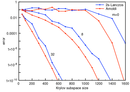
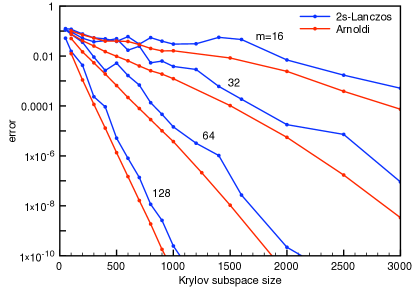
Figure 1: Comparison of the convergence rate for the Arnoldi and the two-sided Lanczos method for a $4^{4}$ (left) and $6^{4}$ (right) lattice, for various deflation sizes.

However, the speed of the short recurrences by far makes up for this as can be seen from Fig. 2, where we show the accuracy as a function of the required CPU-time. The two-sided Lanczos method is clearly more efficient than the Arnoldi method, and the advantage gained by the short recurrences increases as the volume grows. The dotted lines show the time needed to build the basis in the Krylov subspace, while the full lines represent the total CPU-time used by the iterative method (without the deflation time). The construction of the basis is much faster for the two-sided Lanczos method ($\sim Nk$) than in the Arnoldi case ($\sim Nk^{2}$). For the Arnoldi method the time needed to construct the Arnoldi basis is dominating, while for the two-sided Lanczos this time can almost be neglected compared to that needed to compute the sign function of the inner matrix. Methods to boost the computation of the sign function of the inner matrix are the subject of a current study. An additional advantage of the short recurrences is their possible implementation with small memory footprint if a two-pass procedure is used to compute Eq. (19).

Figure 2: Accuracy versus CPU-time (in seconds), on an Intel Core 2 Duo 2.33GHz workstation, for the Arnoldi (red) and the two-sided Lanczos method (blue) for a $4^{4}$ (left) and $6^{4}$ (right) lattice.

To make the method practical for large-scale lattice simulations it will be important to improve the deflation phase, even though first tests on larger lattices ($16^{3}\times 32$) with realistic parameter values seem to indicate that the number of deflated eigenvalues can be taken much smaller than in the $4^{4}$ and $6^{4}$ lattices investigated herein.

The methods discussed above are also currently being tested to compute eigenvalues of the overlap operator. First results are encouraging and clearly show the superiority of the two-sided Lanczos method.

References

- [1] H.B. Nielsen and M. Ninomiya, Phys. Lett. B105 (1981) 219.
- [2] P.H. Ginsparg and K.G. Wilson, Phys. Rev. D25 (1982) 2649.
- [3] R. Narayanan and H. Neuberger, Nucl. Phys. B443 (1995) 305, hep-th/9411108.
- [4] H. Neuberger, Phys. Lett. B417 (1998) 141, hep-lat/9707022.
- [5] J. Bloch and T. Wettig, Phys. Rev. Lett. 97 (2006) 012003, hep-lat/0604020.
- [6] P. Hasenfratz and F. Karsch, Phys. Lett. B125 (1983) 308.
- [7] G. Golub and C.V. Loan, Matrix Computations (The John Hopkins University Press, 1989).
- [8] J. Bloch and T. Wettig, Phys. Rev. D76 (2007) 114511, 0709.4630.
- [9] G. Akemann, J. Bloch, L. Shifrin and T. Wettig, Phys. Rev. Lett. 100 (2008) 032002, 0710.2865.
- [10] C. Gattringer and L. Liptak, Phys. Rev. D76 (2007) 054502, 0704.0092.
- [11] D. Banerjee, R.V. Gavai and S. Sharma, (2008), 0803.3925.
- [12] J. Bloch, A. Frommer, B. Lang and T. Wettig, Comput. Phys. Commun. 177 (2007) 933, 0704.3486.
- [13] T. Breu, A two-sided Lanczos method with deflation for the overlap Dirac operator at nonzero quark chemical potential, Master’s thesis, University of Regensburg, 2007.
- [14] Y. Saad, SIAM Journal on Numerical Analysis 29 (1992) 209.