Pseudospin and Deformation-induced Gauge Field in Graphene

Abstract

The basic properties of $\pi$-electrons near the Fermi level in graphene are reviewed from a point of view of the pseudospin and a gauge field coupling to the pseudospin. The applications of the gauge field to the electron-phonon interaction and to the edge states are reported.

1 Introduction

The electronic properties of a single layer of graphite, graphene, [1, 2, 3] have attracted much attention due to the “relativistic” character of $\pi$-electrons near the Fermi level. The energy band structure of graphene exhibits a linear energy dispersion relation around the two inequivalent, hexagonal corners of the first Brillouin zone in the $k$-space (the K and K’ points). [4, 5] The wavefunction (Hamiltonian) of $\pi$-electrons has two component (a $2\times 2$ matrix) form due to the fact that the unit cell of graphene consists of two carbon atoms (A and B atoms). The effective-mass Hamiltonian of $\pi$-electrons around the K point or the K’ point is given by linear momentum operator, which is relevant to the linear energy dispersion relation of graphene. The effective-mass equation is similar to the massless Dirac equation or the Weyl equation. [6]

The original Dirac equation for an electron has the form

$$i\hbar\frac{\partial}{\partial t}\psi({\bf r},t)=\begin{pmatrix}-c\mbox{\boldmath$\sigma$}\cdot{\hat{\bf p}}&Imc^{2}\cr Imc^{2}&c\mbox{\boldmath$\sigma$}\cdot{\hat{\bf p}}\end{pmatrix}\psi({\bf r},t),$$ (1)

where $c$ is the speed of light, $m$ is the mass of electron, and ${\hat{\bf p}}$ $(=-i\hbar\nabla)$ is the momentum operator. The Hamiltonian is a $4\times 4$ matrix, which is written in terms of the Pauli matrices $\mbox{\boldmath$\sigma$}=(\sigma_{x},\sigma_{y},\sigma_{z})$ and $2\times 2$ identity matrix $I$.  $\psi({\bf r},t)$ of the Dirac equation is a four-component wavefunction, which naturally explains the spin degree of freedom for particle (electron) and the antiparticle (positron). In the massless limit ($m=0$), the Dirac equation is split into two equations of a $2\times 2$ matrix form, that is, the Weyl equations for massless neutrinos. Setting $\psi={}^{t}(\psi_{L},\psi_{R})$ in Eq. (1), we obtain the Weyl equation for $\psi_{R}$ and $\psi_{L}$ as

$$\begin{split}&i\hbar\frac{\partial}{\partial t}\psi_{L}({\bf r},t)=-c\mbox{\boldmath$\sigma$}\cdot{\hat{\bf p}}\psi_{L}({\bf r},t),\\ &i\hbar\frac{\partial}{\partial t}\psi_{R}({\bf r},t)=c\mbox{\boldmath$\sigma$}\cdot{\hat{\bf p}}\psi_{R}({\bf r},t).\end{split}$$ (2)

The two component of each Weyl equation represents the spin degree of freedom.

On the other hand, the effective-mass equations for the K and K’ points of graphene are written as

$$\begin{split}&i\hbar\frac{\partial}{\partial t}\psi^{\rm K}({\bf r},t)=v_{\rm F}\mbox{\boldmath$\sigma$}\cdot{\hat{\bf p}}\psi^{\rm K}({\bf r},t),\\ &i\hbar\frac{\partial}{\partial t}\psi^{\rm K^{\prime}}({\bf r},t)=v_{\rm F}\mbox{\boldmath$\sigma$}^{\prime}\cdot{\hat{\bf p}}\psi^{\rm K^{\prime}}({\bf r},t),\end{split}$$ (3)

where $v_{\rm F}$ is the Fermi velocity, $\mbox{\boldmath$\sigma$}=(\sigma_{x},\sigma_{y})$, $\mbox{\boldmath$\sigma$}^{\prime}=(-\sigma_{x},\sigma_{y})$, and ${\hat{\bf p}}=({\hat{p}}_{x},{\hat{p}}_{y})$. The equation for $\psi^{\rm K}$ of Eq. (3) is similar to the Weyl equation for $\psi_{R}$ of Eq. (2) with $p_{z}=0$ and by substituting $c$ to $v_{\rm F}$. The equation for $\psi^{\rm K^{\prime}}$ is similar to the Weyl equation for $\psi_{L}$ with $p_{z}=0$, the substitution of $c$ to $v_{\rm F}$, and the negative sign in front of $\sigma_{y}$. Although the character of the two component of the effective-mass equations of graphene (A and B atoms) and of the Weyl equation (up spin and down spin) is different from each other, the equation and the resulting solution for given $\sigma_{x}$ and $\sigma_{y}$ are the same. Thus, it is appropriate that the two component structures $\psi_{\rm K}={}^{t}(\psi_{\rm K}^{A},\psi_{\rm K}^{B})$ and $\psi_{\rm K^{\prime}}={}^{t}(\psi_{\rm K^{\prime}}^{A},\psi_{\rm K^{\prime}}^{B})$ of the effective-mass equations for graphene near the Fermi level is referred to as the pseudospin. A pseudospin structure gives a rich variety of interesting physical phenomena of graphene and nanotubes. It is known that absence of a backward scattering of an electron in graphene and carbon nanotubes is relevant to the nature of pseudospin, [7, 8] in which a $2\pi$ rotation of a pseudospin wavefunction around the K point in the two-dimensional Brillouin zone does not gives the original wavefunction but gives minus sign to the wavefunction. The pseudospin in the $k$-space behaves similarly to the real spin in the real space.

The interaction between an electron and an electromagnetic field is given by replacing ${\hat{\bf p}}$ in the Dirac equation with the kinematical momentum ${\hat{}\mbox{\boldmath$\pi$}}={\hat{\bf p}}-e{\bf A}({\bf r})$ where $-e$ is the charge of electron and ${\bf A}({\bf r})$ is a vector potential. The spin of an electron is polarized by a magnetic field, ${\bf B}({\bf r})=\nabla\times{\bf A}({\bf r})$, which can be shown explicitly by the Dirac equation. [6] In the non-relativistic limit, the Dirac equation reduces to the Pauli equation in which the leading interaction between spin and a magnetic field is reduced to the Zeeman term:

$$-\frac{e\hbar}{2m}\mbox{\boldmath$\sigma$}\cdot{\bf B}({\bf r}).$$ (4)

Since the equation for graphene is similar to the Dirac equation, the following question arises; What is the field that polarizes the pseudospin? A magnetic field is a candidate. The same procedure as that in Eq. (4) shows, however, that the pseudospin is not polarized by a magnetic field because the Zeeman term appears with the opposite sign at the K point and at the K’ point as

$$\begin{split}&-\frac{e\hbar}{2m}\mbox{\boldmath$\sigma$}\cdot{\bf B}({\bf r})\ \ ({\rm K}\ {\rm point}),\\ &+\frac{e\hbar}{2m}\mbox{\boldmath$\sigma$}\cdot{\bf B}({\bf r})\ \ ({\rm K^{\prime}}\ {\rm point}).\end{split}$$ (5)

Thus the direction of the pseudospin polarization which is induced at the K point by a magnetic field is opposite to that at the K’ point by the same magnetic field. Thus the pseudospin of graphene is not polarized by ${\bf B}({\bf r})$.  Mathematically, this observation leads us to assume a new gauge field ${\bf A}^{\rm q}({\bf r})$ which has the opposite sign of ${\bf A}^{\rm q}({\bf r})$ at the K point to the K’ point as

$$\begin{split}&i\hbar\frac{\partial}{\partial t}\psi_{\rm K}({\bf r},t)=v_{\rm F}\mbox{\boldmath$\sigma$}\cdot\left({\hat{\bf p}}+{\bf A}^{\rm q}({\bf r})\right)\psi_{\rm K}({\bf r},t),\\ &i\hbar\frac{\partial}{\partial t}\psi_{\rm K^{\prime}}({\bf r},t)=v_{\rm F}\mbox{\boldmath$\sigma$}^{\prime}\cdot\left({\hat{\bf p}}-{\bf A}^{\rm q}({\bf r})\right)\psi_{\rm K^{\prime}}({\bf r},t).\end{split}$$ (8)

Then the corresponding field defined by ${\bf B}^{\rm q}({\bf r})=\nabla\times{\bf A}^{\rm q}({\bf r})$ can polarize the pseudospin because the Zeeman term appears as the same sign for the K and K’ points in this case.

There is an example of the pseudospin-polarized state, that is, a localized state appearing near the zigzag edge of graphene, which is called the edge states. [9] The wavefunction of the edge state has a value only on A atoms when the zigzag edge atoms consist of A atoms. Thus we expect that a field ${\bf B}^{\rm q}({\bf r})$ appears around the edge. We will show that the zigzag edge structure is relevant to a field ${\bf B}^{\rm q}({\bf r})$ which polarizes the pseudospin near the zigzag edge. [10] A gauge field ${\bf A}^{\rm q}({\bf r})$ and a field ${\bf B}^{\rm q}({\bf r})$ is important not only for the localized edge states but also for the extended states. For example, the electron-phonon (el-ph) interaction in graphene can be expressed by ${\bf A}^{\rm q}({\bf r})$, which explains the chirality dependence of the el-ph interaction. [11] In this paper we review our studies performed on the gauge field ${\bf A}^{\rm q}({\bf r})$ by showing that the el-ph interaction and the edge boundary are expressed by ${\bf A}^{\rm q}({\bf r})$.

Here, we would like to mention the relationship between our work and previously published literature on deformation-induced gauge field. Kane and Mele introduced a homogeneous deformation-induced gauge field in the effective-mass theory. [12] The gauge field represents uniform lattice deformations such as uniform bend, twist and curvature of a carbon nanotube. The uniform gauge field for the curvature of a nanotube changes the boundary condition around a tube axis which is given by a generalized Aharanov-Bohm (AB) effect and induces a small energy gap in a chiral metallic carbon nanotube. The curvature-induced mini gap was observed by scanning tunneling spectroscopy (STS) experiment by Ouyang et al. [13] A generalization of the gauge field to a local field is necessary for describing a local lattice deformation. In the previous paper, [14] we generalized the gauge field introduced by Kane and Mele, to include a local lattice deformation of graphene. Further, by defining a deformation-induced magnetic field, we explained the local modulation of the energy band gap, [14] which was observed in the STS measurement for pea-pod (C${}_{6}0$ encapsulated carbon nanotube) by Lee et al. [15]

This paper is organized as follows. In § 2, we derive the effective-mass equations for graphene and define the pseudospin. We show that the pseudospin determines the elastic scattering amplitude of an electron by impurity potentials. In § 3, we derive the effective-mass equation in the presence of the lattice deformation, in which gauge symmetry for ${\bf A}^{\rm q}({\bf r})$ is essential to the time-reversal properties of the el-ph interaction. In § 4, the formulation explained in § 3 is applied to the el-ph interaction for optical and acoustic phonon modes. In § 5, we will discuss the edge state by ${\bf A}^{\rm q}({\bf r})$. In § 6, summary of this paper is given.

2 Effective-mass Theory

In this section, we derive an effective-mass Hamiltonian from the nearest-neighbor tight-binding model for a graphene. The nearest-neighbor tight-binding model is given by

$${\cal H}_{0}=-\gamma_{0}\sum_{i\in{\rm A}}\sum_{a=1,2,3}\left((c_{i+a}^{\rm B})^{\dagger}c_{i}^{\rm A}+(c_{i}^{\rm A})^{\dagger}c_{i+a}^{\rm B}\right),$$ (9)

where $\gamma_{0}$ ($\approx 2.7$ eV) is the nearest-neighbor hopping integral, $c_{i}^{\rm A}$ ($(c_{i}^{\rm A})^{\dagger}$) is the annihilation (creation) operator of $\pi$-electron for A-atom at the position ${\bf r}_{i}$, and $c^{\rm B}_{i+a}$ ($(c^{\rm B}_{i+a})^{\dagger}$) is that for B-atom at ${\bf r}_{i+a}$ $(\equiv{\bf r}_{i}+{\bf R}_{a})$ where ${\bf R}_{a}$ ($a=1,2,3$) are vectors pointing to the three nearest-neighbor B-atoms from an A-atom (see Fig. 1).

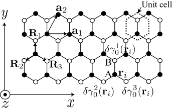
Figure 1: A hexagonal unit cell of graphene consists of A (solid circle) and B (open circle) atoms. ${\bf a}_{1}$ and ${\bf a}_{2}$ are the unit vectors ($a$ denotes the lattice constant: $a\equiv|{\bf a}_{i}|=\sqrt{3}a_{\rm cc}$ where $a_{\rm cc}$ is the C-C bond length.). ${\bf R}_{a}$ ($a=1,2,3$) are vectors pointing to the nearest-neighbor B atoms from an A atom. For the $xyz$ coordinate system, ${\bf R}_{a}$ are written as ${\bf R}_{1}=a_{\rm cc}{\bf e}_{y}$, ${\bf R}_{2}=-(\sqrt{3}/2)a_{\rm cc}{\bf e}_{x}-(1/2)a_{\rm cc}{\bf e}_{y}$, and ${\bf R}_{3}=(\sqrt{3}/2)a_{\rm cc}{\bf e}_{x}-(1/2)a_{\rm cc}{\bf e}_{y}$ where ${\bf e}_{x}$ (${\bf e}_{y}$) is the dimensionless unit vector for the $x$-axis ($y$-axis). Local modulations of the hopping integral are defined by $\delta\gamma^{a}_{0}({\bf r}_{i})$ ($a=1,2,3$) where ${\bf r}_{i}$ ($i\in{\rm A}$) is the position of an A-atom.

We use the Bloch theorem to diagonalize Eq. (9). The Bloch wavefunction with wavevector ${\bf k}$ is defined by

$$|\Psi_{s}^{\bf k}\rangle=\frac{1}{\sqrt{N_{u}}}\sum_{i\in s}e^{i{\bf k}\cdot{\bf r}_{i}}(c^{s}_{i})^{\dagger}|0\rangle\ \ \ (s={\rm A},{\rm B}),$$ (10)

where the sum on $i$ is taken over the crystal, $N_{u}$ is the number of the hexagonal unit cells, and $|0\rangle$ denotes the state of carbon atoms without $\pi$-electrons. The off-diagonal matrix element of ${\cal H}_{0}$ is given by

$$\begin{split}&\langle\Psi_{\rm A}^{\bf k}|{\cal H}_{0}|\Psi_{\rm B}^{\bf k}\rangle=-\gamma_{0}\sum_{a=1,2,3}f_{a}({\bf k})=-\gamma_{0}f({\bf k}),\\ &\langle\Psi_{\rm B}^{\bf k}|{\cal H}_{0}|\Psi_{\rm A}^{\bf k}\rangle=-\gamma_{0}\sum_{a=1,2,3}f_{a}({\bf k})^{*}=-\gamma_{0}f({\bf k})^{*},\end{split}$$ (11)

where $f_{a}({\bf k})\equiv e^{i{\bf k}\cdot{\bf R}_{a}}$ and $f({\bf k})$ is given by [16]

$$f({\bf k})\equiv\sum_{a=1,2,3}f_{a}({\bf k}).$$ (12)

The diagonal matrix element of ${\cal H}_{0}$, $\langle\Psi_{s}^{\bf k}|{\cal H}_{0}|\Psi_{s}^{\bf k}\rangle$, ($s=$A,B) can be taken to be zero. The energy eigenequation is written by a $2\times 2$ matrix form as

$$E({\bf k})\begin{pmatrix}|\Psi_{\rm A}^{\bf k}\rangle\cr|\Psi_{\rm B}^{\bf k}\rangle\end{pmatrix}=-\gamma_{0}\begin{pmatrix}0&f({\bf k})\cr f({\bf k})^{*}&0\end{pmatrix}\begin{pmatrix}|\Psi_{\rm A}^{\bf k}\rangle\cr|\Psi_{\rm B}^{\bf k}\rangle\end{pmatrix}.$$ (13)

The energy band structure of graphene is obtained by solving

$$\det\begin{pmatrix}E({\bf k})&\gamma_{0}f({\bf k})\cr\gamma_{0}f({\bf k})^{*}&E({\bf k})\end{pmatrix}=0,$$ (14)

whose solution is $E({\bf k})=+\gamma_{0}|f({\bf k})|$, ($-\gamma_{0}|f({\bf k})|$) for the conduction (valence) energy band. The conduction energy band and the valence energy band touch with each other at the K point, ${\bf k}_{\rm F}$ ($=(4\pi/3a,0)$), and at the K’ point, $-{\bf k}_{\rm F}$, where $|f({\bf k})|$ vanishes. By expanding $f_{a}({\bf k})$ in Eq. (11) around the wavevector of ${\bf k}_{\rm F}$ (the K point), we obtain

$$f_{a}({\bf k}_{\rm F}+{\bf k})=f_{a}({\bf k}_{\rm F})+if_{a}({\bf k}_{\rm F}){\bf k}\cdot{\bf R}_{a}+\cdots.$$ (15)

Here ${\bf k}$ ($=(k_{x},k_{y})$) is measured from the K point. Using ${\bf k}_{\rm F}=(4\pi/3a,0)$, we get $f_{1}({\bf k}_{\rm F})=1$, $f_{2}({\bf k}_{\rm F})=e^{-i\frac{2\pi}{3}}$, and $f_{3}({\bf k}_{\rm F})=e^{+i\frac{2\pi}{3}}$. Substituting $f_{a}({\bf k}_{\rm F})$ into Eq. (15), we obtain from Eq. (11) that

$$\begin{split}&\langle\Psi_{\rm A}^{{\bf k}_{\rm F}+{\bf k}}|{\cal H}_{0}|\Psi_{\rm B}^{{\bf k}_{\rm F}+{\bf k}}\rangle=\gamma_{0}\frac{3a_{\rm cc}}{2}(k_{x}-ik_{y})+{\cal O}(k^{2}),\\ &\langle\Psi_{\rm B}^{{\bf k}_{\rm F}+{\bf k}}|{\cal H}_{0}|\Psi_{\rm A}^{{\bf k}_{\rm F}+{\bf k}}\rangle=\gamma_{0}\frac{3a_{\rm cc}}{2}(k_{x}+ik_{y})+{\cal O}(k^{2}),\end{split}$$ (16)

where we used $\langle\Psi_{\rm A}^{{\bf k}_{\rm F}}|{\cal H}_{0}|\Psi_{\rm B}^{{\bf k}_{\rm F}}\rangle=-\gamma_{0}f({\bf k}_{\rm F})=0$.

From Eq. (16), we see that Eq. (13) becomes

$$E({\bf k}_{\rm F}+{\bf k})\begin{pmatrix}|\Psi_{\rm A}^{{\bf k}_{\rm F}+{\bf k}}\rangle\cr|\Psi_{\rm B}^{{\bf k}_{\rm F}+{\bf k}}\rangle\end{pmatrix}=\frac{3\gamma_{0}a_{\rm cc}}{2}\begin{pmatrix}0&k_{x}-ik_{y}\cr k_{x}+ik_{y}&0\end{pmatrix}\begin{pmatrix}|\Psi_{\rm A}^{{\bf k}_{\rm F}+{\bf k}}\rangle\cr|\Psi_{\rm B}^{{\bf k}_{\rm F}+{\bf k}}\rangle\end{pmatrix}.$$ (17)

By introducing the Fermi velocity as $v_{\rm F}\equiv\gamma_{0}3a_{\rm cc}/2\hbar$ ($\sim 10^{6}$m/s), the momentum operator $\hat{\bf p}=-i\hbar\nabla$, and the Pauli matrix $\mbox{\boldmath$\sigma$}=(\sigma_{x},\sigma_{y})$, we obtain the effective-mass Hamiltonian near the K point as

$${\cal H}^{\rm K}_{0}=v_{\rm F}\mbox{\boldmath$\sigma$}\cdot\hat{\mathbf{p}}.$$ (18)

${\cal H}^{\rm K}_{0}$ is a $2\times 2$ matrix which operates on the two component wavefunction: $\psi^{\rm K}({\bf r})={}^{t}(\psi^{\rm K}_{\rm A}({\bf r}),\psi^{\rm K}_{\rm B}({\bf r}))$ where $\psi^{\rm K}_{\rm A}({\bf r})$ and $\psi^{\rm K}_{\rm B}({\bf r})$ are the Bloch wavefunction for $\pi$-electrons of the A and B atom in the unit cell. By introducing $\Theta({\bf k})$ which is defined by an angle of ${\bf k}=(k_{x},k_{y})$ measured from the $k_{x}$-axis, then we get $(k_{x},k_{y})\equiv|{\bf k}|(\cos\Theta({\bf k}),\sin\Theta({\bf k}))$, and

$${\cal H}_{0}^{\rm K}=\hbar v_{\rm F}|{\bf k}|\begin{pmatrix}0&e^{-i\Theta({\bf k})}\cr e^{+i\Theta({\bf k})}&0\end{pmatrix}.$$ (19)

The energy eigenvalue of Eq. (19) is given by $\pm v_{\rm F}|{\bf p}|$ and the energy dispersion relation shows a linear dispersion relation near the K point as is known as the Dirac cone. At the K (or K’) point, the valence and conduction bands touch to each other and thus we call the degenerated point as the Dirac point. The eigenstates for $E=+v_{\rm F}|{\bf p}|$ and $E=-v_{\rm F}|{\bf p}|$ are given by

$$\psi^{\rm K}_{c,{\bf k}}({\bf r})=\frac{e^{i{\bf k}\cdot{\bf r}}}{\sqrt{2S}}\begin{pmatrix}e^{-i\Theta({\bf k})/2}\cr e^{+i\Theta({\bf k})/2}\end{pmatrix},\ \ \psi^{\rm K}_{v,{\bf k}}({\bf r})=\frac{e^{i{\bf k}\cdot{\bf r}}}{\sqrt{2S}}\begin{pmatrix}e^{-i\Theta({\bf k})/2}\cr-e^{+i\Theta({\bf k})/2}\end{pmatrix},$$ (20)

which are a conduction band state and a valence band state with the wavevector ${\bf k}$.  In Eq. (20), $S$ denotes the surface area of graphene. In the case of single wall carbon nanotube (SWNT), the $k_{x}$-axis is taken in the circumferential direction on the cylindrical surface and the $k_{y}$-axis is defined by the direction of a zigzag nanotube axis (see the coordinate system in Fig. 1(a)). We see in Eq. (20) that the energy eigenstate for the valence band, $\psi^{\rm K}_{v,{\bf k}}({\bf r})$ is given by $\sigma_{z}\psi^{\rm K}_{c,{\bf k}}({\bf r})$. This is because of a particle-hole symmetry of the Hamiltonian: ${\cal H}^{\rm K}_{0}\sigma_{z}=-\sigma_{z}{\cal H}_{0}^{\rm K}$. 

Similarly, the effective-mass Hamiltonian for the K’ point is given by expanding $f_{a}({\bf k})$ around $-{\bf k}_{\rm F}$ (the K’ point) in Eq. (11) as

$${\cal H}^{\rm K^{\prime}}_{0}=v_{F}\mbox{\boldmath$\sigma$}^{\prime}\cdot\hat{\mathbf{p}},$$ (24)

where $\mbox{\boldmath$\sigma$}^{\prime}\equiv(-\sigma_{x},\sigma_{y})$ and ${\cal H}^{\rm K^{\prime}}_{0}$ operates on a two-component wavefunction: $\psi^{\rm K^{\prime}}({\bf r})={}^{t}(\psi^{\rm K^{\prime}}_{\rm A}({\bf r}),\psi^{\rm K^{\prime}}_{\rm B}({\bf r}))$. The energy eigenstates for the conduction and valence energy band are given, respectively, by

$$\psi^{\rm K^{\prime}}_{c,{\bf k}^{\prime}}({\bf r})=\frac{e^{i{\bf k}^{\prime}\cdot{\bf r}}}{\sqrt{2S}}\begin{pmatrix}e^{+i\Theta({\bf k}^{\prime})/2}\cr-e^{-i\Theta({\bf k}^{\prime})/2}\end{pmatrix},\ \ \psi^{\rm K^{\prime}}_{v,{\bf k}^{\prime}}({\bf r})=\sigma_{z}\psi^{\rm K^{\prime}}_{c,{\bf k}^{\prime}}({\bf r})=\frac{e^{i{\bf k}^{\prime}\cdot{\bf r}}}{\sqrt{2S}}\begin{pmatrix}e^{+i\Theta({\bf k}^{\prime})/2}\cr e^{-i\Theta({\bf k}^{\prime})/2}\end{pmatrix}$$ (25)

where $k^{\prime}_{x}-ik^{\prime}_{y}\equiv|{\bf k}^{\prime}|e^{-i\Theta({\bf k}^{\prime})}$.

The linear energy dispersion relations near the K and K’ points, $E=\pm v_{\rm F}|{\bf p}|$, are contrasted to the non-relativistic energy dispersion relation of $|{\bf p}|^{2}/2m$ where $m$ is the effective-mass of the particle. The effective-mass for graphene can be understood to be zero from the definition of relativistic energy $E=\pm\sqrt{p^{2}c^{2}+m^{2}c^{4}}=\pm c|{\bf p}|$ for $m=0$, where $c$ is substituted to $v_{\rm F}$ ($\sim c/300$). The wavefunction with two components is defined by the “pseudospin”. The pseudospin up (down) state ${}^{t}(1,0)$ (${}^{t}(0,1)$) corresponds to the wavefunction which has a value only on A (B) atoms. As we see in Eq. (20), if we rotate ${\bf k}$ by $2\pi$ around the K point ${\bf k}=0$, that is, $\Theta({\bf k})+2\pi$, then $\psi_{c,\Theta({\bf k})+2\pi}^{\rm K}({\bf r})=-\psi_{c,\Theta({\bf k})}^{\rm K}({\bf r})$, which is the same structure for a real spin under a $2\pi$ rotation in the real space.

Here, we give an example to show that the pseudospin is relevant to a vanishing matrix element for the lowest order backscattering amplitude. [17] When a carrier in the conduction band is denoted by $|{\bf k}c\rangle$, then the matrix element of the backscattering process is written as $\langle{\bf-k}c|{\cal H}_{\rm imp}|{\bf k}c\rangle$. When the impurity potential is long-range compared with the lattice constant, the potential is modeled by a diagonal form and the matrix element becomes

$$\langle{\bf-k}c|{\cal H}_{\rm imp}|{\bf k}c\rangle=\int\frac{d^{2}{\bf r}}{2S}e^{i2{\bf k}\cdot{\bf r}}\begin{pmatrix}e^{+i\Theta(-{\bf k})/2}\cr e^{-i\Theta(-{\bf k})/2}\end{pmatrix}^{t}\begin{pmatrix}V({\bf r})&0\cr 0&V({\bf r})\end{pmatrix}\begin{pmatrix}e^{-i\Theta({\bf k})/2}\cr e^{+i\Theta({\bf k})/2}\end{pmatrix}=0,$$ (26)

where we use Eq. (20) and $\Theta({\bf-k})=\Theta({\bf k})\pm\pi$. This means that the interference between the two component pseudospin makes the back scattering matrix element vanish. In general, there are many impurities in a sample, which gives rise to the Anderson localization in the disordered systems. There is an interesting way to explain the ballistic transport of carbon nanotube even in the many scattering events. [7] For a back scattered wave, we can find a time-reversal scattering wave whose wavefunction has an additional phase shift of $\pi$. The time reversal pair of scattered waves  cancel with each other, which leads to the absence of the backward scattering. [7] This is contrasted with the standard concept that impurity scattering gives rise to the Anderson localization for low-dimensional systems.

3 Gauge Field for a Deformed Graphene

The dynamics of the conducting electrons in graphene materials are different from those of ideal flat graphene, because in the former case, there are shape fluctuations (cylindrical shape, phonon vibration, etc.) that result in the modification of the overlap matrix elements. of nearest-neighbor $\pi$-orbitals and of the on-site potential energy. We refer the modification of the nearest-neighbor hopping integral as the off-site interaction and a shift of the on-site potential energy as the on-site interaction. The modification of the effective-mass equations by the off-site (on-site) interaction is discussed in Sec. 3.1 (Sec. 3.2). We discuss time-reversal symmetry property of the effective-mass equations including the off-site and on-site interactions in Sec. 3.3.

3.1 Off-site interaction

First we consider the perturbation from the off-site interaction in which only off-diagonal matrix element has a non-zero value. A lattice deformation induces a local modification of the nearest-neighbor hopping integral as $-\gamma_{0}\to-\gamma_{0}+\delta\gamma_{0}^{a}({\bf r}_{i})$ ($a=1,2,3$) (see Fig. 1). We define the perturbation ${\cal H}_{1}$ as

$${\cal H}_{1}\equiv\sum_{i\in{\rm A}}\sum_{a=1,2,3}\delta\gamma^{a}_{0}(\mathbf{r}_{i})\left((c_{i+a}^{\rm B})^{\dagger}c_{i}^{\rm A}+(c_{i}^{\rm A})^{\dagger}c_{i+a}^{\rm B}\right).$$ (27)

The off-site matrix element of ${\cal H}_{1}$ with respect to the Bloch wave functions in Eq. (10) with ${\bf k}$ and ${\bf k}+\delta{\bf k}$ is given by

$$\begin{split}&\langle\Psi_{\rm A}^{{\bf k}+\delta{\bf k}}|{\cal H}_{1}|\Psi_{\rm B}^{{\bf k}}\rangle=\frac{1}{N_{u}}\sum_{i\in{\rm A}}\sum_{a=1,2,3}\delta\gamma^{a}_{0}({\bf r}_{i})f_{a}({\bf k})e^{-i\delta{\bf k}\cdot{\bf r}_{i}},\\ &\langle\Psi_{\rm B}^{{\bf k}+\delta{\bf k}}|{\cal H}_{1}|\Psi_{\rm A}^{{\bf k}}\rangle=\frac{1}{N_{u}}\sum_{i\in{\rm A}}\sum_{a=1,2,3}\delta\gamma^{a}_{0}({\bf r}_{i})f_{a}({\bf k})^{*}e^{-i\delta{\bf k}\cdot({\bf r}_{i}+{\bf R}_{a})}.\end{split}$$ (28)

Here we consider the two possible cases for $\delta{\bf k}$. When $\delta{\bf k}$ is sufficiently small compared with the reciprocal lattice vector, ${\bf k}$ near the K (or K’) point is scattered to the ${\bf k^{\prime}}={\bf k}+\delta{\bf k}$ within the region near the K (or K’) point, which we call the intravalley scattering. On the other hand, if $\delta{\bf k}$ is comparable to the distance between the K and K’ points, we expect scattering from K (K’) point to K’ (K) point, which we call the intervalley scattering.

3.1.1 Intravalley Scattering

In the case of intravalley scattering, when ${\bf k}$ is measured from ${\bf k}_{\rm F}$, we get

$$\begin{split}&\langle\Psi_{\rm A}^{{\bf k}_{\rm F}+{\bf k}+\delta{\bf k}}|{\cal H}_{1}|\Psi_{\rm B}^{{\bf k}_{\rm F}+{\bf k}}\rangle=\frac{1}{N_{u}}\sum_{i\in{\rm A}}\sum_{a=1,2,3}\delta\gamma_{a}({\bf r}_{i})f_{a}({\bf k}_{\rm F})e^{-i\delta{\bf k}\cdot{\bf r}_{i}}+{\cal O}(\delta k\delta\gamma_{a}),\\ &\langle\Psi_{\rm B}^{{\bf k}_{\rm F}+{\bf k}+\delta{\bf k}}|{\cal H}_{1}|\Psi_{\rm A}^{{\bf k}_{\rm F}+{\bf k}}\rangle=\frac{1}{N_{u}}\sum_{i\in{\rm A}}\sum_{a=1,2,3}\delta\gamma_{a}({\bf r}_{i})f_{a}({\bf k}_{\rm F})^{*}e^{-i\delta{\bf k}\cdot{\bf r}_{i}}+{\cal O}(\delta k\delta\gamma_{a}),\end{split}$$ (29)

The correction indicated by ${\cal O}(\delta k\delta\gamma_{a})$ in Eq. (29) is negligible when $|\delta{\bf k}|\ll|{\bf k}_{\rm F}|$. Substituting $f_{1}({\bf k}_{\rm F})=1$, $f_{2}({\bf k}_{\rm F})=e^{-i\frac{2\pi}{3}}$ and $f_{3}({\bf k}_{\rm F})=e^{+i\frac{2\pi}{3}}$ into Eq.(29), we get

$$\begin{split}&\langle\Psi_{\rm A}^{{\bf k}_{\rm F}+{\bf k}+\delta{\bf k}}|{\cal H}_{1}|\Psi_{\rm B}^{{\bf k}_{\rm F}+{\bf k}}\rangle=\frac{v_{\rm F}}{N_{u}}\sum_{i\in{\rm A}}\left\{A_{x}^{\rm q}({\bf r}_{i})-iA_{y}^{\rm q}({\bf r}_{i})\right\}e^{-i\delta{\bf k}\cdot{\bf r}_{i}},\\ &\langle\Psi_{\rm B}^{{\bf k}_{\rm F}+{\bf k}+\delta{\bf k}}|{\cal H}_{1}|\Psi_{\rm A}^{{\bf k}_{\rm F}+{\bf k}}\rangle=\frac{v_{\rm F}}{N_{u}}\sum_{i\in{\rm A}}\left\{A_{x}^{\rm q}({\bf r}_{i})+iA_{y}^{\rm q}({\bf r}_{i})\right\}e^{-i\delta{\bf k}\cdot{\bf r}_{i}},\end{split}$$ (30)

where ${\bf A}^{\rm q}({\bf r})=(A_{x}^{\rm q}({\bf r}),A_{y}^{\rm q}({\bf r}))$ is defined by $\delta\gamma^{a}_{0}({\bf r})$ ($a=1,2,3$) as

$$\begin{split}&v_{\rm F}A_{x}^{\rm q}({\bf r})=\delta\gamma^{1}_{0}({\bf r})-\frac{1}{2}\left(\delta\gamma^{2}_{0}({\bf r})+\delta\gamma^{3}_{0}({\bf r})\right),\\ &v_{\rm F}A_{y}^{\rm q}({\bf r})=\frac{\sqrt{3}}{2}\left(\delta\gamma^{2}_{0}({\bf r})-\delta\gamma^{3}_{0}({\bf r})\right).\end{split}$$ (31)

Since the diagonal term vanishes, that is, $\langle\Psi_{s}^{\bf k}|{\cal H}_{1}|\Psi_{s}^{\bf k^{\prime}}\rangle=0$ ($s={\rm A,B}$), Eq. (30) shows that ${\cal H}_{1}$ is expressed by $v_{\rm F}\mbox{\boldmath$\sigma$}\cdot{\bf A}^{\rm q}({\bf r})$ in the effective-mass Hamiltonian. Thus, the total Hamiltonian of a deformed graphene is expressed by

$${\cal H}^{\rm K}_{0}+{\cal H}^{\rm K}_{1}=v_{\rm F}\mbox{\boldmath$\sigma$}\cdot(\hat{\bf p}+{\bf A}^{\rm q}({\bf r})).$$ (32)

Similarly, by expanding $f_{a}({\bf k})$ in Eq. (28) around $-{\bf k}_{\rm F}$ of the K’ point, we find ${\cal H}_{1}$ appears as $-v_{\rm F}\mbox{\boldmath$\sigma$}^{\prime}\cdot{\bf A}^{\rm q}({\bf r})$. Thus, we obtain the effective-mass Hamiltonian for the K’ point as

$${\cal H}^{\rm K^{\prime}}_{0}+{\cal H}^{\rm K^{\prime}}_{1}=v_{\rm F}\mbox{\boldmath$\sigma$}^{\prime}\cdot(\hat{\mathbf{p}}-\mathbf{A}^{\rm q}({\bf r})).$$ (33)

The corresponding Schrödinger equation for Eqs (32) and (33) are given in Eq. (3). [14]

Thus, the off-site interaction can be included in the effective-mass equations as a gauge field, ${\bf A}^{\rm q}({\bf r})$. We call ${\bf A}^{\rm q}({\bf r})$ the deformation-induced gauge field and distinguish it from the electromagnetic gauge field ${\bf A}({\bf r})$. [14] ${\cal H}_{0}+{\cal H}_{1}$ does not break time-reversal symmetry even tough the ${\bf A}^{\rm q}({\bf r})$ appears as a gauge field, because the sign in front of ${\bf A}^{\rm q}({\bf r})$ is opposite to each other for the K and K’ points. This contrasts with the fact that ${\bf A}({\bf r})$ (magnetic field) violates time-reversal symmetry because the sign in front of ${\bf A}({\bf r})$ is the same for the K and K’ points as ${\hat{\bf p}}\to{\hat{\bf p}}-e{\bf A}({\bf r})$. The time-reversal symmetry will be discussed in detail in Sec. 3.3. The rotation of ${\bf A}^{\rm q}({\bf r})$ or the deformation-induced magnetic field is defined by ${\bf B}^{\rm q}({\bf r})=\nabla\times{\bf A}({\bf r})$ as

$$B^{\rm q}_{z}({\bf r})=\frac{\partial A_{y}^{\rm q}({\bf r})}{\partial x}-\frac{\partial A_{x}^{\rm q}({\bf r})}{\partial y}.$$ (34)

The direction of $B^{\rm q}_{z}(\mathbf{r})$ is perpendicular to the graphene plane ${\bf B}^{\rm q}(\mathbf{r})=(0,0,B^{\rm q}_{z}(\mathbf{r}))$. The deformation-induced magnetic field changes the energy band structure, which will be shown in § 5. The $B^{\rm q}_{z}({\bf r})$ couples with the pseudospin through $\sigma_{z}$ term. This is shown by taking the square of the effective-mass equations, as we see in Eqs. (6) and (7),

$$\begin{split}&E^{2}\psi^{\rm K}({\bf r})=v_{\rm F}^{2}\left\{(\hat{\mathbf{p}}+\mathbf{A}^{\rm q}(\mathbf{r}))^{2}+\hbar B_{z}^{\rm q}(\mathbf{r})\sigma_{z}\right\}\psi^{\rm K}({\bf r}),\\ &E^{2}\psi^{\rm K^{\prime}}({\bf r})=v_{\rm F}^{2}\left\{(\hat{\mathbf{p}}-\mathbf{A}^{\rm q}(\mathbf{r}))^{2}+\hbar B^{\rm q}_{z}(\mathbf{r})\sigma_{z}\right\}\psi^{\rm K^{\prime}}({\bf r}),\end{split}$$ (35)

where $B^{\rm q}_{z}({\bf r})\sigma_{z}$ terms modify the direction of the pseudospin to the direction opposite to $B^{\rm q}_{z}({\bf r})$ in order to decrease the energy for the both K and K’ points. Here let us stress a notable difference between $B^{\rm q}_{z}({\bf r})$ and the usual magnetic field, $B_{z}({\bf r})$. For $B_{z}^{\rm q}({\bf r})$, a uniform magnetic field along the z-axis over a sample is possible to realize the uniform spin polarization (the Zeeman term). However, since $B^{\rm q}_{z}({\bf r})$ is generated by the modification of $\gamma_{0}$, the field $B^{\rm q}_{z}({\bf r})$ appears only near the defect region without periodic symmetry such as the zigzag edge [10] which gives local polarization of pseudospin. In general, when a graphene sample contains an equal number of A and B atoms to each other, we have

$$\int_{S}B^{\rm q}_{z}({\bf r})d^{2}{\bf r}=0,$$ (36)

where $S$ denotes an integral for a whole sample.

3.1.2 Intervalley Scattering

Next, we consider the matrix element of ${\cal H}_{1}$ for the intervalley scattering. Let us define the wave vector of a Bloch state near the K point; ${\bf k}_{\rm F}+{\bf k}$ and that of another Bloch state near the K’ point; $-{\bf k}_{\rm F}+{\bf k^{\prime}}$ ($|{\bf k}|,|{\bf k^{\prime}}|\ll|{\bf k}_{\rm F}|$), then the matrix element from the K’ to K points is written by using Eq. (28) as

$$\langle\Psi_{\rm A}^{{\bf k}_{\rm F}+{\bf k}}|{\cal H}_{1}|\Psi_{\rm B}^{-{\bf k}_{\rm F}+{\bf k}^{\prime}}\rangle =\frac{1}{N_{u}}\sum_{i\in{\rm A}}\sum_{a=1,2,3}\delta\gamma^{a}_{0}(\mathbf{r}_{i})f_{a}({\bf k}_{\rm F})^{*}e^{-i2{\bf k}_{\rm F}\cdot{\bf r}_{i}}e^{i({\bf k^{\prime}}-{\bf k})\cdot{\bf r}_{i}}e^{i{\bf k^{\prime}}\cdot{\bf R}_{a}}$$

$$\simeq\frac{1}{N_{u}}\sum_{i\in{\rm A}}\sum_{a=1,2,3}\delta\gamma^{a}_{0}(\mathbf{r}_{i})f_{a}({\bf k}_{\rm F})^{*}e^{-i2{\bf k}_{\rm F}\cdot{\bf r}_{i}}e^{i({\bf k^{\prime}}-{\bf k})\cdot{\bf r}_{i}}$$

$$=\frac{v_{\rm F}}{N_{u}}\sum_{i\in{\rm A}}\left\{A_{x}^{\rm q}({\bf r}_{i})+iA_{y}^{\rm q}({\bf r}_{i})\right\}e^{-i2{\bf k}_{\rm F}\cdot{\bf r}_{i}}e^{i({\bf k^{\prime}}-{\bf k})\cdot{\bf r}_{i}},$$ (37)

and

$$\langle\Psi_{\rm B}^{{\bf k}_{\rm F}+{\bf k}}|{\cal H}_{1}|\Psi_{\rm A}^{-{\bf k}_{\rm F}+{\bf k}^{\prime}}\rangle =\frac{1}{N_{u}}\sum_{i\in{\rm A}}\sum_{a=1,2,3}\delta\gamma^{a}_{0}(\mathbf{r}_{i})f_{a}({\bf k}_{\rm F})^{*}e^{-i2{\bf k}_{\rm F}\cdot{\bf r}_{i}}e^{i({\bf k^{\prime}}-{\bf k})\cdot{\bf r}_{i}}e^{-i{\bf k}\cdot{\bf R}_{a}}$$

$$\simeq\frac{1}{N_{u}}\sum_{i\in{\rm A}}\sum_{a=1,2,3}\delta\gamma^{a}_{0}(\mathbf{r}_{i})f_{a}({\bf k}_{\rm F})^{*}e^{-i2{\bf k}_{\rm F}\cdot{\bf r}_{i}}e^{i({\bf k^{\prime}}-{\bf k})\cdot{\bf r}_{i}}$$

$$=\frac{v_{\rm F}}{N_{u}}\sum_{i\in{\rm A}}\left\{A_{x}^{\rm q}({\bf r}_{i})+iA_{y}^{\rm q}({\bf r}_{i})\right\}e^{-i2{\bf k}_{\rm F}\cdot{\bf r}_{i}}e^{i({\bf k^{\prime}}-{\bf k})\cdot{\bf r}_{i}}.$$ (38)

In Eqs. (37) and (38), from the first line of the right-hand side to the second line, we approximate $e^{i{\bf k^{\prime}}\cdot{\bf R}_{a}}\approx 1$ and $e^{-i{\bf k}\cdot{\bf R}_{a}}\approx 1$ since we consider the case of $|{\bf k}^{\prime}|\ll|{\bf k}_{\rm F}|$ and $|{\bf k}|\ll|{\bf k}_{\rm F}|$. Equations (37) and (38) show that the deformation-induced gauge field ${\bf A}^{\rm q}({\bf r})$ (Eq. (31)) can be applied to the matrix element for intervalley scattering, too. It is noted that Eqs. (37) and (38) are identical to each other up to the leading term. The matrix elements from the K point to the K’ point are given by replacing ${\bf k}_{\rm F}$ by $-{\bf k}_{\rm F}$ in Eqs. (37) and (38) as

$$\begin{split}&\langle\Psi_{\rm A}^{-{\bf k}_{\rm F}+{\bf k}^{\prime}}|{\cal H}_{1}|\Psi_{\rm B}^{{\bf k}_{\rm F}+{\bf k}}\rangle=\frac{v_{\rm F}}{N_{u}}\sum_{i\in{\rm A}}\left\{A_{x}^{\rm q}({\bf r}_{i})-iA_{y}^{\rm q}({\bf r}_{i})\right\}e^{+i2{\bf k}_{\rm F}\cdot{\bf r}_{i}}e^{-i({\bf k^{\prime}}-{\bf k})\cdot{\bf r}_{i}},\\ &\langle\Psi_{\rm B}^{-{\bf k}_{\rm F}+{\bf k}^{\prime}}|{\cal H}_{1}|\Psi_{\rm A}^{{\bf k}_{\rm F}+{\bf k}}\rangle=\frac{v_{\rm F}}{N_{u}}\sum_{i\in{\rm A}}\left\{A_{x}^{\rm q}({\bf r}_{i})-iA_{y}^{\rm q}({\bf r}_{i})\right\}e^{+i2{\bf k}_{\rm F}\cdot{\bf r}_{i}}e^{-i({\bf k^{\prime}}-{\bf k})\cdot{\bf r}_{i}}.\end{split}$$ (39)

In the effective-mass model, the intervalley scattering appears as the off-diagonal terms in a $4\times 4$ matrix:

$$E\begin{pmatrix}\psi^{\rm K}({\bf r})\cr\psi^{\rm K^{\prime}}({\bf r})\end{pmatrix}=v_{\rm F}\begin{pmatrix}\mbox{\boldmath$\sigma$}\cdot(\hat{\bf p}+{\bf A}^{\rm q}({\bf r}))&\phi^{\rm q}({\bf r})\sigma_{x}\cr\phi^{\rm q}({\bf r})^{*}\sigma_{x}&\mbox{\boldmath$\sigma$}^{\prime}\cdot(\hat{\bf p}-{\bf A}^{\rm q}({\bf r}))\end{pmatrix}\begin{pmatrix}\psi^{\rm K}({\bf r})\cr\psi_{\rm K^{\prime}}({\bf r})\end{pmatrix},$$ (40)

where we define a deformation-induced complex scalar field $\phi({\bf r})$

$$\phi^{\rm q}({\bf r})\equiv(A_{x}^{\rm q}({\bf r})+iA_{y}^{\rm q}({\bf r}))e^{-i2{\bf k}_{\rm F}\cdot{\bf r}}.$$ (41)

When ${\bf A}^{\rm q}({\bf r})$ is a smooth function of ${\bf r}$, the effect of intervalley scattering by the complex scalar field $\phi^{\rm q}({\bf r})$ can be neglected because $\phi^{\rm q}({\bf r})$ becomes a rapidly oscillating function of ${\bf r}$ due to the factor $e^{-i2{\bf k}_{\rm F}\cdot{\bf r}}$, and the value of matrix element between the K and K’ points becomes negligible, too. On the other hand, when ${\bf A}^{\rm q}({\bf r})$ is a rapidly oscillating function of ${\bf r}$, $\phi^{\rm q}({\bf r})$ becomes a smooth function of ${\bf r}$ and the matrix element between the K and K’ points is not negligible. For example, phonon modes at the K point contribute to the intervalley scattering. Since the vibrational amplitude of the K point phonon modes are proportional to $e^{-i{\bf k}_{\rm F}\cdot{\bf r}_{i}}$, ${\bf A}^{\rm q}({\bf r}_{i})$ has the same periodicity of $e^{+2i{\bf k}_{\rm F}\cdot{\bf r}_{i}}$ where we use the fact $e^{+3i{\bf k}_{\rm F}\cdot{\bf r}_{i}}=1$. Then, $\phi^{\rm q}({\bf r}_{i})$ would behave as a constant in the real space.

3.2 On-site interaction

Now we consider the on-site interaction by a defect of the crystal. A lattice deformation gives rise to not only a change of the transfer integral between A and B atoms but also a change of the potential at the A (B) atom $\phi_{A}$ ($\phi_{B}$) which we call the off-site and on-site deformation potential, respectively. We denote the on-site deformation potential by a $2\times 2$ matrix for $\psi={}^{t}(\psi^{\rm K},\psi^{\rm K^{\prime}})$

$${\cal H}_{\rm on}=\begin{pmatrix}\phi_{\rm A}({\bf r}_{i})&0\cr 0&\phi_{\rm B}({\bf r}_{i}+{\bf R}_{1})\end{pmatrix}.$$ (42)

Let the displacement vector of A-atom at ${\bf r}_{i}$ is ${\bf u}_{\rm A}({\bf r}_{i})$ and that of B-atom at ${\bf r}_{j}$ is ${\bf u}_{\rm B}({\bf r}_{j})$, then the deformation potential of A-atom at ${\bf r}_{i}$, $\phi_{\rm A}({\bf r}_{i})$, is induced by the relative displacements of three nearest neighbor B-atoms from the A-atom (${\bf u}_{\rm B}({\bf r}_{i}+{\bf R}_{a})-{\bf u}_{\rm A}({\bf r}_{i})$) as

$$\phi_{\rm A}({\bf r}_{i})=\frac{g_{\rm on}}{\ell a_{\rm cc}}\sum_{a=1,2,3}{\bf R}_{a}\cdot\left({\bf u}_{\rm B}({\bf r}_{i}+{\bf R}_{a})-{\bf u}_{\rm A}({\bf r}_{i})\right),$$ (43)

where $g_{\rm on}$ denotes gradient of the atomic potential at ${\bf r}_{i}$, and $\ell$ denotes $3a_{\rm cc}/2$. Here we assume that $|{\bf u}_{\rm B}({\bf r}_{i}+{\bf R}_{a})-{\bf u}_{\rm A}({\bf r}_{i})|\ll a_{\rm cc}$ and that $\phi_{\rm A}({\bf r}_{i})$ depends linearly on the relative displacement vector.

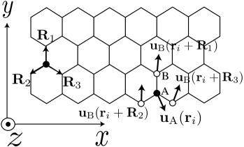
Figure 2: Displacements of B-atoms at ${\bf r}_{i}+{\bf R}_{a}$ ($a=1,2,3$), ${\bf u}_{\rm B}({\bf r}_{i}+{\bf R}_{a})$, give rise to a deformation potential at A-atom of ${\bf r}_{i}$.

By expanding ${\bf u}_{\rm B}({\bf r}_{i}+{\bf R}_{2})$ as ${\bf u}_{\rm B}({\bf r}_{i}+{\bf R}_{2})={\bf u}_{\rm B}({\bf r}_{i}+{\bf R}_{1})+(({\bf R}_{2}-{\bf R}_{1})\cdot\nabla){\bf u}_{\rm B}({\bf r}_{i}+{\bf R}_{1})+\cdots$ and ${\bf u}_{\rm B}({\bf r}_{i}+{\bf R}_{3})$ as ${\bf u}_{\rm B}({\bf r}_{i}+{\bf R}_{3})={\bf u}_{\rm B}({\bf r}_{i}+{\bf R}_{1})+(({\bf R}_{3}-{\bf R}_{1})\cdot\nabla){\bf u}_{\rm B}({\bf r}_{i}+{\bf R}_{1})+\cdots$, we see that Eq. (43) can be approximated by

$$\phi_{\rm A}({\bf r}_{i})=g_{\rm on}\nabla\cdot{\bf u}_{\rm B}({\bf r}_{i}+{\bf R}_{1})+\cdots,$$ (44)

where we have used $\sum_{a=1,2,3}{\bf R}_{a}=0$. It is noted that a general expression for the deformation potential, Eq. (44), is valid in the case that ${\bf u}_{\rm B}({\bf r})$ is a smooth function of ${\bf r}$. When this is not the case, we have to use Eq. (43). In the continuous limit, we may use ${\bf r}$ to represent the positions of both A and B atoms in the unit cell, then we have $\phi_{\rm A}({\bf r})=g_{\rm on}\nabla\cdot{\bf u}_{\rm B}({\bf r})+\cdots$. Similarly, the deformation potential of B-site of ${\bf r}_{i}+{\bf R}_{1}$ is given by

$$\phi_{\rm B}({\bf r}_{i}+{\bf R}_{1})=\frac{g_{\rm on}}{\ell a_{\rm cc}}\sum_{a=1,2,3}-{\bf R}_{a}\cdot\left({\bf u}_{\rm A}({\bf r}_{i}+{\bf R}_{1}-{\bf R}_{a})-{\bf u}_{\rm B}({\bf r}_{i}+{\bf R}_{1})\right).$$ (45)

By using ${\bf u}_{\rm A}({\bf r}_{i}+{\bf R}_{1}-{\bf R}_{2})={\bf u}_{\rm A}({\bf r}_{i})+(({\bf R}_{1}-{\bf R}_{2})\cdot\nabla){\bf u}_{\rm A}({\bf r}_{i})+\cdots$ and ${\bf u}_{\rm A}({\bf r}_{i}+{\bf R}_{1}-{\bf R}_{3})={\bf u}_{\rm A}({\bf r}_{i})+(({\bf R}_{1}-{\bf R}_{3})\cdot\nabla){\bf u}_{\rm A}({\bf r}_{i})+\cdots$, we see that Eq. (45) can be approximated by

$$\phi_{\rm B}({\bf r}_{i}+{\bf R}_{1})=g_{\rm on}\nabla\cdot{\bf u}_{\rm A}({\bf r}_{i})+\cdots.$$ (46)

Thus, for the intravalley scattering, we may rewrite Eq. (42) using Eqs. (44) and (46) as

$${\cal H}_{\rm on}=g_{\rm on}\begin{pmatrix}\nabla\cdot{\bf u}_{\rm B}({\bf r})&0\cr 0&\nabla\cdot{\bf u}_{\rm A}({\bf r})\end{pmatrix}+\cdots.$$ (47)

According to the result of density-functional theory by Porezag et al., [18, 19] we will use the parameter for $g_{\rm on}$ ($=$17eV). For the later discussion of el-ph interaction of acoustic

$${\bf s}({\bf r})\equiv\frac{{\bf u}_{\rm A}({\bf r})+{\bf u}_{\rm B}({\bf r})}{2},$$ (48)

and optical

$${\bf u}({\bf r})\equiv{\bf u}_{\rm B}({\bf r})-{\bf u}_{\rm A}({\bf r}),$$ (49)

phonon modes, we rewrite Eq. (47) using the Pauli matrices as

$${\cal H}_{\rm on}=\frac{g_{\rm on}}{2}I\nabla\cdot({\bf u}_{\rm A}({\bf r})+{\bf u}_{\rm B}({\bf r}))+\frac{g_{\rm on}}{2}\sigma_{z}\nabla\cdot({\bf u}_{\rm B}({\bf r})-{\bf u}_{\rm A}({\bf r})).$$ (50)

Comparing with the expressions for ${\bf A}^{\rm q}({\bf r})$ and $\phi^{\rm q}({\bf r})$ in Eqs. (31) and (41), and for Eq. (50), the effective-mass Hamiltonian of the defect of the crystal is given by

$${\cal H}=v_{\rm F}\begin{pmatrix}{\cal H}^{\rm K}&v_{\rm F}\phi^{\rm q}({\bf r})\sigma_{x}\cr v_{\rm F}\phi^{\rm q}({\bf r})^{*}\sigma_{x}&{\cal H}^{\rm K^{\prime}}\end{pmatrix},$$ (51)

where we define

$$\begin{split}&{\cal H}^{\rm K}=v_{\rm F}\mbox{\boldmath$\sigma$}\cdot(\hat{\bf p}+{\bf A}^{\rm q}({\bf r}))+g_{\rm on}I\nabla\cdot{\bf s}({\bf r})+\frac{g_{\rm on}}{2}\sigma_{z}\nabla\cdot{\bf u}({\bf r}),\\ &{\cal H}^{\rm K^{\prime}}=v_{\rm F}\mbox{\boldmath$\sigma$}^{\prime}\cdot(\hat{\bf p}-{\bf A}^{\rm q}({\bf r}))+g_{\rm on}I\nabla\cdot{\bf s}({\bf r})+\frac{g_{\rm on}}{2}\sigma_{z}\nabla\cdot{\bf u}({\bf r}).\end{split}$$ (52)

3.3 Time-reversal and pseudospin symmetries

Here we show that ${\bf A}^{\rm q}({\bf r})$ keeps time-reversal symmetry of graphene system. The time-reversal operation, ${\cal T}$, is defined by exchanging the K point and the K’ point, and taking a complex conjugation of the four component wavefunction as

$${\cal T}\begin{pmatrix}\psi^{\rm K}({\bf r})\cr\psi^{\rm K^{\prime}}({\bf r})\end{pmatrix}=\begin{pmatrix}\psi^{\rm K^{\prime}}({\bf r})^{*}\cr\psi^{\rm K}({\bf r})^{*}\end{pmatrix},\ {\rm where}\ {\cal T}=\begin{pmatrix}0&I\cr I&0\end{pmatrix}K$$ (53)

and $K$ is the complex conjugate operator. In order to check that Eq. (53) is time-reversal operation, it is useful to introduce the vector potential for electro-magnetism, ${\bf A}({\bf r})$, into the effective-mass Hamiltonian as

$${\cal H}=v_{\rm F}\begin{pmatrix}\mbox{\boldmath$\sigma$}\cdot(\hat{\bf p}+{\bf A}^{\rm q}({\bf r})-e{\bf A}({\bf r}))&\phi^{\rm q}({\bf r})\sigma_{x}\cr\phi^{\rm q}({\bf r})^{*}\sigma_{x}&\mbox{\boldmath$\sigma$}^{\prime}\cdot(\hat{\bf p}-{\bf A}^{\rm q}({\bf r})-e{\bf A}({\bf r}))\end{pmatrix}.$$ (54)

Then the electromagnetic current operator, ${\bf J}({\bf r})$, is given by

$${\bf J}({\bf r})=\frac{\partial{\cal H}}{\partial{\bf A}({\bf r})}=-ev_{\rm F}\begin{pmatrix}\mbox{\boldmath$\sigma$}&0\cr 0&\mbox{\boldmath$\sigma$}^{\prime}\end{pmatrix}.$$ (55)

Using ${\cal T}$ in Eq. (53), we can show that

$${\cal T}^{-1}{\bf J}({\bf r}){\cal T}=-{\bf J}({\bf r}),$$ (56)

where we have used $K^{-1}\mbox{\boldmath$\sigma$}K=-\mbox{\boldmath$\sigma$}^{\prime}$ and $K^{-1}\mbox{\boldmath$\sigma$}^{\prime}K=-\mbox{\boldmath$\sigma$}$. The negative sign on the right-hand side of Eq. (56) shows that Eq. (53) is time-reversal operation.

When we apply ${\cal T}$ to the wavefunction of Eq. (40), we get

$$E\begin{pmatrix}\psi^{\rm K^{\prime}}({\bf r})^{*}\cr\psi^{\rm K}({\bf r})^{*}\end{pmatrix}=v_{\rm F}\begin{pmatrix}\mbox{\boldmath$\sigma$}\cdot(\hat{\bf p}+{\bf A}^{\rm q}({\bf r}))&\phi^{\rm q}({\bf r})\sigma_{x}\cr\phi^{\rm q}({\bf r})^{*}\sigma_{x}&\mbox{\boldmath$\sigma$}^{\prime}\cdot(\hat{\bf p}-{\bf A}^{\rm q}({\bf r}))\end{pmatrix}\begin{pmatrix}\psi^{\rm K^{\prime}}({\bf r})^{*}\cr\psi^{\rm K}({\bf r})^{*}\end{pmatrix}.$$ (57)

By taking the complex conjugation (c.c.) of the first row of Eq. (57), we get

$$E\psi^{\rm K^{\prime}}({\bf r})^{*}=v_{\rm F}\mbox{\boldmath$\sigma$}\cdot(\hat{\bf p}+{\bf A}^{\rm q}({\bf r}))\psi^{\rm K^{\prime}}({\bf r})^{*}+v_{\rm F}\phi^{\rm q}({\bf r})\sigma_{x}\psi^{\rm K}({\bf r})^{*}$$

$$\stackrel{{\scriptstyle\rm c.c.}}{{\to}}E\psi^{\rm K^{\prime}}({\bf r})=v_{\rm F}\mbox{\boldmath$\sigma$}^{\prime}\cdot(\hat{\bf p}-{\bf A}^{\rm q}({\bf r}))\psi^{\rm K^{\prime}}({\bf r})+v_{\rm F}\phi^{\rm q}({\bf r})^{*}\sigma_{x}\psi^{\rm K}({\bf r})$$ (58)

where we have used $\mbox{\boldmath$\sigma$}^{*}=-\mbox{\boldmath$\sigma$}^{\prime}$ and $\hat{\bf p}^{*}=-\hat{\bf p}$. Similarly, by taking the complex conjugation of the second row of Eq. (57), we get

$$E\psi^{\rm K}({\bf r})^{*}=v_{\rm F}\phi^{\rm q}({\bf r})^{*}\sigma_{x}\psi^{\rm K^{\prime}}({\bf r})^{*}+v_{\rm F}\mbox{\boldmath$\sigma$}^{\prime}\cdot(\hat{\bf p}-{\bf A}^{\rm q}({\bf r}))\psi^{\rm K}({\bf r})^{*}$$

$$\stackrel{{\scriptstyle\rm c.c.}}{{\to}}E\psi^{\rm K}({\bf r})=v_{\rm F}\phi^{\rm q}({\bf r})\sigma_{x}\psi^{\rm K^{\prime}}({\bf r})+v_{\rm F}\mbox{\boldmath$\sigma$}\cdot(\hat{\bf p}+{\bf A}^{\rm q}({\bf r}))\psi^{\rm K}({\bf r}).$$ (59)

The equations in the last lines of Eqs. (58) and (59) are nothing but the second and first row of Eq. (40), respectively. Therefore, Eq. (54) (or Eq. (40)) is symmetric under the time-reversal transformation (when ${\bf A}({\bf r})=0$).

When $\phi^{\rm q}({\bf r})=0$, it is useful to define an operation ${\cal S}$ that transforms the electron of ${\bf k}$ to that of ${\bf-k}$ within the same valley. The operation ${\cal S}$ is defined by

$${\cal S}\begin{pmatrix}\psi^{\rm K}({\bf r})\cr\psi^{\rm K^{\prime}}({\bf r})\end{pmatrix}=\begin{pmatrix}\sigma_{y}\psi^{\rm K}({\bf r})^{*}\cr\sigma_{y}\psi^{\rm K^{\prime}}({\bf r})^{*}\end{pmatrix},\ {\rm where}\ {\cal S}=\begin{pmatrix}I&0\cr 0&I\end{pmatrix}\sigma_{y}K.$$ (60)

This operation is referred to as effective time-reversal symmetry or special time-reversal symmetry because we obtain ${\cal S}^{-1}{\bf J}({\bf r}){\cal S}=-{\bf J}({\bf r})$ for the special case of $\phi^{\rm q}({\bf r})=0$, ${\bf A}^{\rm q}({\bf r})=0$, and ${\bf A}({\bf r})=0$. By applying Eq. (60) to the wavefunction of Eq. (40), we get for the first row as

$$E\sigma_{y}\psi^{\rm K}({\bf r})^{*}=v_{\rm F}\mbox{\boldmath$\sigma$}\cdot(\hat{\bf p}+{\bf A}^{\rm q}({\bf r}))\sigma_{y}\psi^{\rm K}({\bf r})^{*}+v_{\rm F}\phi^{\rm q}({\bf r})\sigma_{x}\sigma_{y}\psi^{\rm K^{\prime}}({\bf r})^{*}$$

$$\stackrel{{\scriptstyle\sigma_{y}}}{{\to}}E\psi^{\rm K}({\bf r})^{*}=v_{\rm F}\mbox{\boldmath$\sigma$}^{\prime}\cdot(\hat{\bf p}+{\bf A}^{\rm q}({\bf r}))\psi^{\rm K}({\bf r})^{*}-v_{\rm F}\phi^{\rm q}({\bf r})\sigma_{x}\psi^{\rm K^{\prime}}({\bf r})^{*}$$

$$\stackrel{{\scriptstyle\rm c.c.}}{{\to}}E\psi^{\rm K}({\bf r})=v_{\rm F}\mbox{\boldmath$\sigma$}\cdot(\hat{\bf p}-{\bf A}^{\rm q}({\bf r}))\psi^{\rm K}({\bf r})-v_{\rm F}\phi^{\rm q}({\bf r})^{*}\sigma_{x}\psi^{\rm K^{\prime}}({\bf r})$$ (61)

Here, from the first line to the second line, we multiplied $\sigma_{y}$ to both sides and used $\sigma_{y}\mbox{\boldmath$\sigma$}\sigma_{y}=\mbox{\boldmath$\sigma$}^{\prime}$. To get the last line, we took the complex conjugation of the second line and used $(\mbox{\boldmath$\sigma$}^{\prime})^{*}=-\mbox{\boldmath$\sigma$}$ and $\hat{\bf p}^{*}=-\hat{\bf p}$. The special operation ${\cal S}$ becomes a symmetry when ${\bf A}^{\rm q}({\bf r})=0$. Note that ${\bf A}^{\rm q}({\bf r})=0$ results in $\phi^{\rm q}({\bf r})=0$ because of Eq. (41).

We comment on the definition of the time-reversal operation and the on-site interaction. The transformation defined by Eq. (53) does not contain any Pauli spin matrix since time-reversal symmetry has nothing to do with the pseudospin degree of freedom. It is also noted that the pseudospin degree of freedom ($\sigma_{y}$ in Eq. (60)) is necessary to define the special symmetry of Eq. (60). Even in the presence of the on-site deformation potential of Eq. (42), the time-reversal symmetry of Eq. (53) is valid since Eq. (53) does not contain the Pauli spin matrix. However, the special symmetry of Eq. (60) is lost when Eq. (42) is not symmetric about the sublattice. [20] Namely, when we take into account a non-vanishing $\sigma_{z}$ term of Eq. (50) for Eq. (61), the symmetry of Eq. (60) is broken even when ${\bf A}^{\rm q}({\bf r})=0$.

4 Electron-Phonon Interaction

In this section, we apply the ${\bf A}^{\rm q}({\bf r})$ for phonon mode to describe the el-ph interaction. There are six phonon modes in graphene: in-plane longitudinal optical/acoustic mode (LO/LA), in-plane tangential optical/acoustic mode (iTO/iTA), and out-of-plane tangential optical/acoustic mode (oTO/oTA). [16] We consider long wavelength in-plane optical phonon modes; the LO and iTO phonon modes near the $\Gamma$ point. Using Eqs. (31) and (50), we will derive ${\bf A}^{\rm q}({\bf r})$ and ${\cal H}_{\rm on}$ for the el-ph interaction of the LO/iTO modes. The material in this section has been used to analyze the LO/iTO phonon frequency shift in metallic SWNTs. [11] The phonon frequency shift is observed as a function of the Fermi energy (the Kohn anomaly) in the Raman spectroscopy experiments. [21, 22, 23, 24, 25, 26]

4.1 $\Gamma$ point optical phonon modes

The el-ph interaction originates from a change of the atomic potential due to a vibration of a carbon atom. In Fig. 3, we show a change of the atomic potential whereby $\delta\gamma^{a}_{0}({\bf r})$ is induced. The atomic potential whose origin is located at ${\bf r}$ is denoted by solid curves and the shifted potential whose origin is located at ${\bf r}+\Delta{\bf r}$ is plotted by dashed curves. The deformation potential is given by $\Phi({\bf r}+\Delta{\bf r})-\Phi({\bf r})=\Delta{\bf r}\cdot\nabla\Phi({\bf r})+\cdots$, which gives rise to matrix element between the $\pi$-electron at A-atom and the $\pi$-electron at B-atom as $\langle\Psi_{\rm B}({\bf r}+{\bf R}_{a})|\nabla\Phi({\bf r})|\Psi_{\rm A}({\bf r})\rangle\cdot({\bf R}_{a}/a_{\rm cc})$. In this paper we denote this matrix element as $g_{\rm off}/\ell$, that is, $\langle\Psi_{\rm B}({\bf r}+{\bf R}_{a})|\nabla\Phi({\bf r})|\Psi_{\rm A}({\bf r})\rangle\cdot({\bf R}_{a}/a_{\rm cc})=g_{\rm off}/\ell$. According to density functional calculation by Porezag et al., [18] we have $g_{\rm off}/\ell=3.0$eV/Å [27, 19] where $\ell\equiv 3a_{\rm cc}/2=2.13$Å.

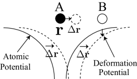
Figure 3: The atomic potential of a carbon atom at ${\bf r}$ is denoted by solid curves and the shifted potential of the carbon atom at ${\bf r}+\Delta{\bf r}$ is plotted by dashed curves. The deformation potential at the B atom is given by $\Phi({\bf r}+\Delta{\bf r})-\Phi({\bf r})=\Delta{\bf r}\cdot\nabla\Phi({\bf r})+\cdots$. The deformation potential gives rise to a scattering of a $\pi$-electron from A-atom to the B-atom as $\langle\Psi_{\rm B}({\bf r}+{\bf R}_{a})|\nabla\Phi({\bf r})|\Psi_{\rm A}({\bf r})\rangle\cdot({\bf R}_{a}/a_{\rm cc})$.

When $\Delta{\bf r}={\bf u}({\bf r})$ (${\bf u}({\bf r})$ is defined in Eq. (49)), the change of the C-C bond-length is given by ${\bf u}({\bf r})\cdot({\bf R}_{a}/a_{\rm cc})$. Thus $\delta\gamma^{a}_{0}({\bf r})$ for the LO and TO modes is given by

$$\delta\gamma^{a}_{0}({\bf r})=\frac{g_{\rm off}}{\ell}{\bf u}({\bf r})\cdot\frac{{\bf R}_{a}}{a_{\rm cc}}.$$ (62)

By putting Eq. (62) into Eq. (31), we obtain

$$\begin{split}&v_{\rm F}A^{\rm q}_{x}({\bf r})=\frac{g_{\rm off}}{\ell a_{\rm cc}}{\bf u}({\bf r})\cdot\left({\bf R}_{1}-\frac{{\bf R}_{2}+{\bf R}_{3}}{2}\right),\\ &v_{\rm F}A^{\rm q}_{y}({\bf r})=\frac{g_{\rm off}}{\ell a_{\rm cc}}\frac{\sqrt{3}}{2}{\bf u}({\bf r})\cdot\left({\bf R}_{2}-{\bf R}_{3}\right).\end{split}$$ (63)

Because ${\bf R}_{1}-({\bf R}_{2}+{\bf R}_{3})/2=\ell{\bf e}_{y}$ and $\sqrt{3}/2({\bf R}_{2}-{\bf R}_{3})=-\ell{\bf e}_{x}$ (see the caption of Fig. 1), we can rewrite Eq. (63) by ${\bf A}^{\rm q}({\bf r})$ as

$$v_{\rm F}(A^{\rm q}_{x}({\bf r}),A^{\rm q}_{y}({\bf r}))=\frac{g_{\rm off}}{a_{\rm cc}}(u_{y}({\bf r}),-u_{x}({\bf r})),$$ (64)

where $u_{x}({\bf r})\equiv{\bf u}({\bf r})\cdot{\bf e}_{x}$ and $u_{y}({\bf r})\equiv{\bf u}({\bf r})\cdot{\bf e}_{y}$. [28] For the on-site el-ph interaction of Eq. (50), we can neglect the term which is proportional to $\sigma_{0}$ since the LO and TO optical phonon modes satisfy ${\bf u}_{\rm A}({\bf r})=-{\bf u}_{\rm B}({\bf r})$. Then, we get

$${\cal H}_{\rm on}=\frac{g_{\rm on}}{2}\sigma_{z}\nabla\cdot{\bf u}({\bf r}).$$ (65)

The resulting effective-mass Hamiltonian for the K point and K’ point become

$$\begin{split}&{\cal H}^{\rm K}=v_{\rm F}\mbox{\boldmath$\sigma$}\cdot(\hat{\bf p}+{\bf A}^{\rm q}({\bf r}))+\frac{g_{\rm on}}{2}\sigma_{z}\nabla\cdot{\bf u}({\bf r}),\\ &{\cal H}^{\rm K^{\prime}}=v_{\rm F}\mbox{\boldmath$\sigma$}^{\prime}\cdot(\hat{\bf p}-{\bf A}^{\rm q}({\bf r}))+\frac{g_{\rm on}}{2}\sigma_{z}\nabla\cdot{\bf u}({\bf r}),\end{split}$$ (66)

where ${\bf A}^{\rm q}({\bf r})$ is given by Eq. (64). Putting Eq. (64) into Eq. (34), we see in Eq. (66) that $\nabla\cdot{\bf u}({\bf r})$ is proportional to the deformation induced magnetic field since

$$\nabla\cdot{\bf u}({\bf r})=-\frac{v_{\rm F}a_{\rm cc}}{g_{\rm off}}B^{\rm q}_{z}({\bf r}).$$ (67)

Thus, if $B_{z}^{\rm q}({\bf r})\neq 0$, the energy spectrum for an electron has a local energy gap around $E_{\rm F}$ because the terms proportional to $\sigma_{z}$ in the Hamiltonian Eq. (66) work as time dependent mass term.  However, the optical phonon mode does not generate a static (time independent) energy gap because ${\bf u}({\bf r})$ is oscillating as a function of time as ${\bf u}({\bf r})\cos(\omega t)$ so that the time average of $B_{z}({\bf r})$ field vanishes. However, the energy gap can be oscillating as a function of time when the vibration of atoms is coherent in the space.

Next we consider an out-of-plane TO (oTO) phonon mode. The oTO phonon eigenvector is pointing in the direction of perpendicular to the 2D plane and does not give rise to a first order, in-plane bond-length change. Thus, the off-site and on-site el-ph coupling for the oTO mode are negligible as compared with those for in-plane LO and TO modes.

4.1.1 Phonon softening for ${\bf q}=0$ LO/iTO phonon mode

For a uniform $(u_{x},u_{y})$ in the real space, that is, for the LO and TO modes with the phonon wave vector ${\bf q}={\bf 0}$, the el-ph interaction for the LO and TO phonon modes is given only by ${\bf A}^{\rm q}$ in Eq. (66) since $\nabla\cdot{\bf u}({\bf r})=0$. For the $\Gamma$ point optical phonon modes, we consider a virtual electron-hole pair creation by the el-ph interaction, which contributes to the phonon frequency shift in second-order perturbation theory (see Fig. 4(a)). The phonon frequency shift as a function of the Fermi energy has been observed in Raman spectroscopy for graphene [21, 22] and metallic nanotubes. [23, 24, 25, 26]

The el-ph matrix element for the electron-hole pair generation near the K point is given from Eqs. (20) and (64) by

$$\langle{\rm eh}({\bf k})|{\cal H}_{1}^{\rm K}|\omega\rangle =\int(\psi^{\rm K}_{c,{\bf k}}({\bf r}))^{*}v_{\rm F}\mbox{\boldmath$\sigma$}\cdot{\bf A}^{\rm op}\psi^{\rm K}_{v,{\bf k}}({\bf r})d^{2}{\bf r}$$

$$=\frac{g_{\rm off}}{2a_{\rm cc}}\begin{pmatrix}e^{+i\frac{\Theta({\bf k})}{2}}\cr e^{-i\frac{\Theta({\bf k})}{2}}\end{pmatrix}^{t}\begin{pmatrix}0&u_{y}+iu_{x}\cr u_{y}-iu_{x}&0\end{pmatrix}\begin{pmatrix}e^{-i\frac{\Theta({\bf k})}{2}}\cr-e^{+i\frac{\Theta({\bf k})}{2}}\end{pmatrix}.$$ (68)

Let us introduce the angle $\alpha$ between vector ${\bf u}=(u_{x},u_{y})$ and the $x$-axis, then by putting $u_{x}=u\cos\alpha$ and $u_{y}=u\sin\alpha$ ($u_{x}+iu_{y}=ue^{i\alpha}$) into Eq. (68) we obtain

$$\langle{\rm eh}({\bf k})|{\cal H}^{\rm K}_{1}|\omega_{\alpha}\rangle=-ig_{\rm off}\frac{u}{a_{\rm cc}}\cos(\Theta({\bf k})-\alpha).$$ (69)

The el-ph matrix element for the electron-hole pair generation near the K’ point, $\langle{\rm eh}({\bf k})|{\cal H}^{\rm K^{\prime}}_{1}|\omega_{\alpha}\rangle$, is the same as Eq. (69). In Eq. (69), $\alpha$ depends on the LO and TO modes in the case of SWNTs, while $\alpha$ can not be defined uniquely in the case of flat graphene. Let us consider the case of a zigzag SWNT. Then, we denote $x$ ($y$) as a coordinate around (along) the axis as shown in Fig. 1(b). In this case, ${\bf u}=(u_{x},0)$ ($\alpha=0$) is assigned to the TO phonon mode while ${\bf u}=(0,u_{y})$ ($\alpha=\pi/2$) is assigned to the LO phonon mode. By calculating Eq. (69) for the TO mode with $\alpha=0$ and for the LO mode with $\alpha=\pi/2$, we get

$$\begin{split}&\langle{\rm eh}({\bf k})|{\cal H}_{1}^{\rm K}|\omega_{\rm TO}\rangle=-ig_{\rm off}\frac{u}{a_{\rm cc}}\cos\Theta({\bf k}),\\ &\langle{\rm eh}({\bf k})|{\cal H}_{1}^{\rm K}|\omega_{\rm LO}\rangle=-ig_{\rm off}\frac{u}{a_{\rm cc}}\sin\Theta({\bf k}).\end{split}$$ (70)

For a “metallic” zigzag SWNT without the curvature effect, [29, 30] we obtain $\Theta({\bf k})=\pm\pi/2$ for a metallic energy band with $k_{x}=0$ (see Fig. 4(b)). Then, Eq. (70) tells us that only the LO mode gives rise to a non-vanishing el-ph matrix element and the TO mode does not contribute to the electron-hole pair creation. The amplitude for an electron-hole pair creation depends strongly on the curvature effect which shifts the relative position of the cutting line from $k_{x}=0$ (see Fig. 4(b)). When the curvature effect is taken into account, $\cos\Theta({\bf k})=k_{x}/(k_{x}^{2}+k_{y}^{2})^{1/2}$ is nonzero due to $k_{x}\neq 0$. Thus, the low energy electron-hole pair can couple to the TO phonon mode and the matrix element becomes maximum when $k_{y}=0$. On the other hand, the high energy electron-hole pair still decouples to the TO phonon mode since $\cos\Theta({\bf k})\to 0$ for $|k_{y}|\gg|k_{x}|$. This leads to a phonon frequency hardening for the TO phonon mode of a zigzag nanotube when the Fermi energy is located near the Dirac point. [11]

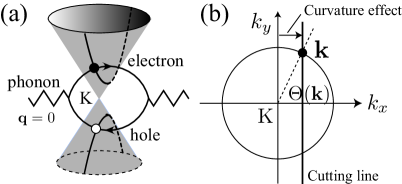
Figure 4: (a) An electron-hole pair on the cutting line near the K point is excited by the $\Gamma$ point phonon mode (${\bf q}=0$). The intermediate electron-hole pair state contributes to the phonon frequency shift. (b) The $k_{x}$ ($k_{y}$) axis corresponds to the zigzag SWNT circumferential (axis) direction. The amplitude for an electron-hole pair creation (Eq. (70)) depends strongly on the relative position of the cutting line from the K point. If the cutting line crosses the K point, then the angle $\Theta({\bf k})$ ($\equiv\arctan(k_{y}/k_{x})$) takes $\pi/2$ ($-\pi/2$) values for $k_{y}>0$ ($k_{y}<0$). In this case, the LO mode strongly couples to an electron-hole pair, while the TO mode is decoupled from the electron-hole pair.

The description of deformation induced gauge field for a lattice deformation (Eq. (31)) is useful to show the appearance of the curvature-induced mini energy gap in metallic zigzag SWNTs. [12] For a zigzag SWNT, we have $\delta\gamma^{1}_{0}=0$ and $\delta\gamma^{2}_{0}=\delta\gamma^{3}_{0}\neq 0$ from the rotational symmetry around the tube axis (see Fig. 1). Then, using Eqs. (31), we get that $A_{x}^{\rm q}=-\delta\gamma_{0}^{2}/v_{\rm F}$ and $A_{y}^{\rm q}=0$ as the curvature effect. The cutting line of $k_{x}=0$ for the metallic zigzag nanotube is shifted by a finite constant value of $A_{x}^{\rm q}$ because of the AB effect for the deformation-induced gauge field ${\bf A}^{\rm q}({\bf r})$. This explains the appearance of the curvature-induced mini energy gap,

$$E_{\rm gap}=\frac{60({\rm meV}\cdot{\rm nm}^{2})}{d_{t}^{2}},$$ (71)

where $d_{t}$ is the diameter of a metallic zigzag SWNT.

4.1.2 ${\bf q}\neq 0$, LO/iTO mode

The description of the el-ph interaction as a gauge field ${\bf A}^{\rm q}({\bf r})$ can be extended to show the decoupling between the TO mode with ${\bf q}\neq 0$ and the electrons using a gauge symmetry argument. [11] The TO phonon mode with ${\bf q}\neq 0$ does not change the area of the hexagonal lattice but instead gives rise to a shear deformation for the hexagonal unit cell of graphene. Thus, the TO mode (${\bf u}_{\rm TO}({\bf r})$) satisfies

$$\nabla\cdot{\bf u}_{\rm TO}({\bf r})=0,\ \ \ \ \nabla\times{\bf u}_{\rm TO}({\bf r})\neq 0.$$ (72)

Thus, the on-site deformation potential is zero in Eq. (66). Using Eqs. (64) and (72), we see that the deformation-induced magnetic field, $B^{\rm q}_{z}({\bf r})$, becomes zero instead the divergence of ${\bf A}^{\rm q}({\bf r})$ exists, which are

$$\begin{split}&(\nabla\times{\bf A}^{\rm q}({\bf r}))\cdot{\bf e}_{z}=B^{\rm q}_{z}({\bf r})=-\frac{g_{\rm off}}{v_{\rm F}a_{\rm cc}}\nabla\cdot{\bf u}_{\rm TO}({\bf r})=0,\\ &\nabla\cdot{\bf A}^{\rm q}({\bf r})=\frac{g_{\rm off}}{v_{\rm F}a_{\rm cc}}(\nabla\times{\bf u}_{\rm TO}({\bf r}))\cdot{\bf e}_{z}\neq 0.\end{split}$$ (73)

In this case, ${\bf A}^{\rm q}({\bf r})$ can be represented by the gradient of a scalar function, $\Psi_{a}({\bf r})$, as ${\bf A}^{\rm q}({\bf r})=\nabla\Psi_{a}({\bf r})$. Since we can choose a ${\bf A}^{\rm q}({\bf r})=0$ gauge in Eq. (66) by a redefinition of the phase of the wavefunction as $\psi^{\rm K}({\bf r})\to\exp(-i\Psi_{a}({\bf r})/\hbar)\psi^{\rm K}({\bf r})$ and $\psi^{\rm K^{\prime}}({\bf r})\to\exp(+i\Psi_{a}({\bf r})/\hbar)\psi^{\rm K^{\prime}}({\bf r})$, [14] the ${\bf A}^{\rm q}({\bf r})$ field in Eq. (66) disappears for the TO mode with ${\bf q}\neq 0$. This explains why the TO mode with ${\bf q}\neq 0$ completely decouples from the electrons and that only the TO mode with ${\bf q}=0$ couples with electrons. In this sense, the TO phonon mode at the $\Gamma$ point is anomalous since the el-ph interaction for the TO mode can not be eliminated by a phase of the wavefunction. On the other hand, the LO phonon mode with ${\bf q}\neq 0$ changes the area of the hexagonal unit cell while it does not give rise to a shear deformation. Thus, the LO mode (${\bf u}_{\rm LO}({\bf r})$) satisfies

$$\nabla\cdot{\bf u}_{\rm LO}({\bf r})\neq 0,\ \ \ \ \nabla\times{\bf u}_{\rm LO}({\bf r})=0.$$ (74)

Using Eqs. (64) and (74), we see that the LO mode gives rise to a deformation-induced magnetic field as

$$B_{z}^{\rm q}({\bf r})\neq 0,\ \ \ \nabla\cdot{\bf A}^{\rm q}({\bf r})=0.$$ (75)

Since a magnetic field changes the energy band structure of electrons through the mass term, the LO mode near the $\Gamma$ point (with ${\bf q}\neq 0$) is important for electronic energy spectrum.

5 Edge States of graphene

Finally, we give two examples of lattice deformation along a line in graphene as shown in Fig. 5(a) and (b) whose field $B^{\rm q}_{z}({\bf r})$ can polarize the pseudospin. In Fig. 5(a), we modify the hopping integral at the dotted line of $y=0$, so that $\delta\gamma_{0}^{1}(\mathbf{r})\neq 0$ at $y=0$ and $\delta\gamma_{0}^{2}(\mathbf{r})=\delta\gamma_{0}^{3}(\mathbf{r})=0$. From Eq. (31), we obtain $v_{F}\mathbf{A}^{\rm q}(y)=(\delta\gamma_{0}^{1}(y),0)$. In Fig. 5(b), the hopping integral along the dotted line at $x=0$ (precisely, $x=0_{+}$ or $x=0_{-}$) is changed as $\delta\gamma_{0}^{1}(\mathbf{r})=0$ and $\delta\gamma_{0}^{2}(\mathbf{r})=\delta\gamma_{0}^{3}(\mathbf{r})\neq 0$ at $x=0$. We obtain $v_{F}\mathbf{A}^{\rm q}(x)=(-\delta\gamma_{0}^{2}(x),0)$ for this case. Figure 5(a) and (b) correspond to the generation of the zigzag edge and the armchair edge in the limit of a strong perturbation, respectively, if we take $\delta\gamma_{0}^{1}=\gamma_{0}$ and $\delta\gamma_{0}^{2}=\delta\gamma_{0}^{3}=\gamma_{0}$ for the hopping integral at the two lines. The behavior of the electronic structure for the two cases are completely different from each other, which we show by calculating the deformation-induced magnetic field. In the case of Fig. 5(a), we have a finite deformation-induced magnetic field $B^{\rm q}_{z}({\bf r})\neq 0$ near the line at $y=0$. The deformation-induced magnetic field $B^{\rm q}_{z}(y)$ is negative at $y<0$ as illustrated by $\otimes$ and is positive at $y>0$ as $\odot$. On the other hand, in the case of Fig. 5(b), the deformation-induced magnetic field is zero. The gauge field which gives zero magnetic field can be removed from Hamiltonian by a gauge transformation, which is discussed in the previous section. The deformation-induced magnetic field accounts for the presence of so-called edge states only at the zigzag edge, which is shown as below. As we show in § 1, the edge state is a localized wavefunction near the zigzag edge in which the pseudospin of the edge state is perfectly polarized. This means that the amplitude of the wavefunction has a value only on either A or B atoms.

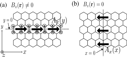
Figure 5: Local deformation along a line and corresponding deformation-induced gauge field ${\bf A}^{\rm q}({\bf r})$ are shown by arrows in (a) zigzag and (b) armchair edge. In (a), ${\bf A}^{\rm q}({\bf r})$ gives a finite deformation-induced magnetic field $B_{z}^{\rm q}({\bf r})$ (flux) illustrated by $\odot$ and $\otimes$ while no deformation-induced magnetic field is present in (b).

We will derive the edge states from the effective-mass model with the gauge field of Fig. 5(a). [10] Before going into the details, let us first outline the story. We will show that there are localized pseudospin-polarized states in the energy spectrum and the energy dispersion appears at $p_{x}>0$ shown as the two solid lines in Fig. 6(b). The velocity for the energy dispersion becomes small with increasing the gauge field and it becomes zero when the gauge field is sufficiently strong which corresponds to the zigzag edge. This result of the effective-mass model can reproduce the result of the tight-binding (TB) lattice model as shown in Fig. 6(c),(d) and (e), [10] where the TB lattice model is defined by an adiabatic parameter $c$ as $\delta\gamma_{0}^{1}(y=0)=c\gamma_{0}$ in Eq. (27). Here $c=0$ and $c=1$ correspond to no deformation and the zigzag edge, respectively.

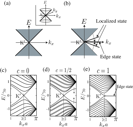
Figure 6: (a) Band structure $(k_{x},E)$ around the K’ point of the effective-mass model without the deformation-induced gauge field and (b) that with the gauge field along the $x$-axis. The shaded regions in (a) and (b) represent the spectrum of extended states for different $k_{y}$. The (two-dimensional) dispersion relation around the K’ point for graphene without the deformation gives two cones (representing the linear $k$ dispersion) whose apex is the K’ point as is shown in the inset of (a). The band structure of (a) is a one-dimensional projection (onto $k_{y}$ plane) of the linear $k$ dispersion. In (b), the energy dispersion for the localized state is represented by solid lines. When the bonds at $y=0$ become disconnected ($c=1$) and zigzag edges appear, the energy eigenvalues of the localized state converge to zero ($E\to 0$) for any $k_{x}(>0)$ and forms a flat energy band of edge state. Using the TB model, we plot the band structure for an undeformed graphene in (c), for a zigzag ribbon in (e), and for a graphene with weakened hopping integral for the C-C bonds at $y=0$ in (d). $k_{x}a$ in (c), (d) and (e) is the wave vector parallel to the $x$-axis and $k_{x}a=2\pi/3$ is the K’ point.

We assume that $\mathbf{A}^{\rm q}(\mathbf{r})$ of Fig. 5(a) is quite localized within $|y|<\xi_{g}$, that is, $\mathbf{A}^{\rm q}(\mathbf{r})=(A_{x}^{\rm q}(y),0)$ and $A_{x}^{\rm q}(y)=0$ for $|y|\geq\xi_{g}$ in Eq. (33), where $\xi_{g}$ is a length of the order of lattice spacing. We parameterize the localized energy eigenstate as

$$\psi^{\rm K^{\prime}}_{E}(\mathbf{r})=N^{\prime}\exp(ik_{x}x)e^{-G(y)}\begin{pmatrix}e^{+g(y)}\cr e^{-g(y)}\end{pmatrix},$$ (76)

where $N^{\prime}$ is a normalization constant. The pseudospin polarization is represented by $g(y)$, and the wave vector $k_{x}$ is a good quantum number because of the translational symmetry along the $x$-axis. In the direction of $y$, we assume a localized nature of the wavefunction which was obtained by TB calculation. Putting Eq. (76) to the energy eigenequation, ${\cal H}^{\rm K^{\prime}}\psi^{\rm K^{\prime}}_{E}(\mathbf{r})=E\psi^{\rm K^{\prime}}_{E}(\mathbf{r})$, we obtain

$$\begin{split}&p_{x}-A_{x}^{\rm q}(y)-\hbar\frac{d}{dy}\left(G(y)+g(y)\right)=-\frac{E}{v_{F}}e^{+2g(y)},\\ &p_{x}-A_{x}^{\rm q}(y)+\hbar\frac{d}{dy}\left(G(y)-g(y))\right)=-\frac{E}{v_{F}}e^{-2g(y)}.\end{split}$$ (77)

By summing and subtracting the both sides of Eq. (77), we rewrite the energy eigenequation as

$$\begin{split}&p_{x}-A_{x}^{\rm q}(y)-\hbar\frac{dg(y)}{dy}=-\frac{E}{v_{F}}\cosh(2g(y)),\\ &\hbar\frac{dG(y)}{dy}=\frac{E}{v_{F}}\sinh(2g(y)).\end{split}$$ (78)

Since we are considering a localized solution around the $x$-axis, we assume $G(y)\sim|y|/\xi$ where $\xi$ $(>0)$ is the localization length. When $G(y)\sim|y|/\xi$, the solution of the second equation of Eq. (78) is given by

$$g(y)=\left\{\begin{array}[]{@{\,}ll}-\frac{1}{2}\sinh^{-1}\left(\frac{\hbar v_{F}}{\xi E}\right)&(y\leq-\xi_{g}),\\ +\frac{1}{2}\sinh^{-1}\left(\frac{\hbar v_{F}}{\xi E}\right)&(y\geq\xi_{g}).\end{array}\right.$$ (81)

The functions $G(y)$ and $g(y)$ are schematically shown in Fig. 7(a) and (b), respectively. The sign of $g(y)$ changes across the $x$-axis; the sign change of $g(y)$ means that the pseudospin direction changes at the $x$-axis. The change of pseudospin is induced by the gauge field $A_{x}^{\rm q}(y)$. To see this, we integrate the first equation of Eq. (78) from $y=-\xi_{g}$ to $\xi_{g}$, and we get the following relation

$$-\int_{-\xi_{g}}^{\xi_{g}}\frac{dg(y)}{dy}dy=\frac{1}{\hbar}\int_{-\xi_{g}}^{\xi_{g}}A_{x}^{\rm q}(y)dy.$$ (82)

We have neglected other terms, since they are proportional to $\xi_{g}$ and become zero in the limit of $\xi_{g}=0$. By putting Eq. (81) to Eq. (82), we find

$$-\sinh^{-1}\left(\frac{\hbar v_{F}}{\xi E}\right)=\frac{1}{\hbar}\int_{-\xi_{g}}^{\xi_{g}}A_{x}^{\rm q}(y)dy.$$ (83)

When the right-hand side of Eq. (83) is large, we obtain from Eq. (81) that $g(y)\gg 0$ for $y\leq-\xi_{g}$ and $g(y)\ll 0$ for $y\geq\xi_{g}$. In this case, the localized state is a pseudospin-up state $\psi^{\rm K}_{E}(\mathbf{r})\propto{}^{t}(1,0)$ for $y\leq-\xi_{g}$ and a pseudospin-down state $\psi^{\rm K}_{E}(\mathbf{r})\propto{}^{t}(0,1)$ for $y\geq\xi_{g}$. Thus, a strong gauge field at the $x$-axis makes pseudospin-polarized localized states. Since the polarization of the pseudospin means that the wave function has amplitude only A (or B) atoms, this result is consistent with the result by the TB model for the edge state. [9] We understand that the edge state is a pseudospin polarized and localized state in the real space which is induced by the deformation-induced magnetic field of the ${\bf A}^{\rm q}({\bf r})$ along the $x$-axis.

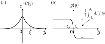
Figure 7: (a) The amplitude of the wave function, $\exp(-G(y))$, of a localized state whose localization length is $\xi$. (b) The pseudo-spin modulation part, $g(y)$. From Eq. (81), $g(y)$ is a constant for $|y|\geq\xi_{g}$, and abruptly changes across the $x$-axis ($y=0$).

Let us now calculate $E$ and $\xi$. To this end, we use the first equation of Eq. (78) for $|y|\geq\xi_{g}$ and obtain

$$\frac{E}{v_{F}}=\frac{-p_{x}}{\cosh\left(\displaystyle\frac{1}{\hbar}\int_{-\xi_{g}}^{\xi_{g}}A_{x}^{\rm q}(y)dy\right)}.$$ (84)

Moreover, using Eq. (83), we get

$$\frac{\hbar}{\xi}=p_{x}\tanh\left(\displaystyle\frac{1}{\hbar}\int_{-\xi_{g}}^{\xi_{g}}A_{x}^{\rm q}(y)dy\right).$$ (85)

In addition to this localized state, there is another localized state for the same $p_{x}$ with the same $\xi$ but with an opposite sign of $E$. This results from a particle-hole symmetry of the Hamiltonian; $\sigma_{z}{\cal H}^{\rm K^{\prime}}\sigma_{z}=-{\cal H}^{\rm K^{\prime}}$. By the particle-hole symmetry operation, the wave function is transformed as $\psi^{\rm K^{\prime}}_{-E}(\mathbf{r})=\sigma_{z}\psi^{\rm K^{\prime}}_{E}(\mathbf{r})$.

The normalization condition of the wave function requires that $\xi$ should be positive, which restricts the value of $p_{x}$ to $p_{x}>0$ in Eq. (85). In fact, when $A_{x}^{\rm q}(y)$ is positive, Eq. (85) means that the localized states appear only at $p_{x}>0$ around the K’ point. This is the reason why the localized states appear in the energy spectrum only in one side around the K’ point as shown in Fig. 6(b). On the other hand, in the case of the K point the Hamiltonian is expressed by Eq. (32). Because of the different signs in front of $\mathbf{A}^{\rm q}(\mathbf{r})$ of Eqs. (32) and (33), a similar argument gives $p_{x}<0$ for the edge states around the K point. Furthermore, when $(1/\hbar)\int_{-\xi_{g}}^{\xi_{g}}A_{x}^{\rm q}(y)dy\gg 0$, $E$ in Eq.(84) becomes zero. The zero energy eigenvalue between the K and K^′ points in the band structure corresponds to the flat energy band of the edge state. [9] When $A_{x}^{\rm q}(y)$ is negative ($A_{x}^{\rm q}(y)\ll 0$), a flat energy band appears in the opposite side: $p_{x}<0$ around the K’ point and $p_{x}>0$ around the K point. This condition, $A_{x}^{\rm q}(y)\ll 0$, corresponds to the Klein’s edges [31] which are obtained by removing A or B atoms out of the zigzag edges having A or B atoms. Calculated result by the TB model with the Klein’s edges [31] is thus analytically explained by ${\bf A}^{\rm q}({\bf r})$.

There are also extended states in addition to the edge states. The energy dispersion relation of extended states can be obtained as $(E/v_{F})^{2}=p_{x}^{2}+p_{y}^{2}$, by setting $G(y)\sim-ip_{y}y/\hbar$ ($|y|\geq\xi_{g}$) in Eqs.(76) and (78) where $p_{y}$ is a real number. The calculated energy bands are given by $|E|>v_{F}|p_{x}|$, shown as a shaded region in Fig. 6(b). It also agrees well with the TB calculation shown in Fig. 6(e). Since $1-\tanh^{2}x=1/\cosh^{2}x$, we see that the energy dispersion relation of the localized state between $E$ and $\xi$ becomes

$$\left(\frac{E}{v_{F}}\right)^{2}=p_{x}^{2}-\left(\frac{\hbar}{\xi}\right)^{2},\ \ (|y|\geq\xi_{g}),$$ (86)

which is the same as the linear dispersion relation $(E/v_{F})^{2}=p_{x}^{2}+p_{y}^{2}$ if one replaces $p_{y}$ with $i(\hbar/\xi)$. Thus One can then regard the localized state as a state with a complex wavenumber.

We have shown that three basic properties of the edge states, i.e., the pseudospin polarization, the dependence on the momentum, and the flat energy band, obtained previously by the TB model, [9] can be explained analytically in terms of the gauge field. In order to compare the present theory with the TB model quantitatively, we have performed a TB calculation for the geometry of Fig. 5(a) with setting $\delta\gamma_{0}^{1}=c\gamma_{0}$. In Figs. 6(c), 6(d) and 6(e), we plot the band structure for $c=0$, $c=1/2$, and $c=1$. Comparing these figures with the results of the continuous model, one can find an exact correspondence between the TB model and continuous model. Moreover, we analytically find [10]

$$\begin{split}&\frac{|E|}{v_{F}}=\frac{|p_{x}|}{\cosh(-\ln(1-c))}+{\cal O}(lp_{x}^{2}/\hbar),\\ &\frac{\hbar}{\xi}=p_{x}\tanh(-\ln(1-c))+{\cal O}(lp_{x}^{2}/\hbar),\end{split}$$ (87)

for localized states around the K’ point. Thus, by comparing Eq. (87) with Eqs. (84) and (85), we conclude that the TB model and the continuous model agree with each other near the K’ point ($p_{x}l/\hbar\ll 1$), by the following relationship

$$\frac{1}{\hbar}\int_{-\xi_{g}}^{\xi_{g}}A_{x}^{\rm q}(y)dy=-\ln(1-c).$$ (88)

The right-hand side diverges when $c\to 1$, which reproduces the flat energy band ($E\to 0$) in Eq. (84) and gives $\xi/\hbar=p_{x}^{-1}$ in Eq. (85). When $c\to 0$, we have $\frac{1}{\hbar}\int_{-\xi_{g}}^{\xi_{g}}A_{x}^{\rm q}(y)dy\simeq c$, which confirms Eq. (31) that is derived by assuming a weak perturbation for $\delta\gamma_{0}^{a}({\bf r})$. 

By considering the edge state using the effective-mass model, we found that the deformation-induced gauge field ($\mathbf{A}^{\rm q}(\mathbf{r})$) and magnetic field ($B^{\rm q}_{z}(\mathbf{r})$) explain basic properties of the edge state. It is summarized as follows:
(1) The gauge field can generate the edge state in energy spectrum, depending on the gauge field direction. Let $\mathbf{e}_{\parallel}$ the unit vector along the edge and $A^{\rm q}_{\parallel}(\mathbf{r})\equiv\mathbf{A}^{\rm q}(\mathbf{r})\cdot\mathbf{e}_{\parallel}$, the edge state appears if the gauge field has a component parallel to the edge: $A^{\rm q}_{\parallel}(\mathbf{r})\neq 0$. This explains the presence (absence) of the edge state near the zigzag (armchair) edge.
(2) The edge states are pseudospin polarized states. The direction of the pseudospin polarization is determined by the direction or sign of $B^{\rm q}_{z}(\mathbf{r})$.
(3) The direction of the gauge field, namely, $A^{\rm q}_{\parallel}(\mathbf{r})>0$ or $A^{\rm q}_{\parallel}(\mathbf{r})<0$, is vital for the edge states, since it determines the energy dispersion and wave vectors which allow the edge states.
(4) The flat energy band of edge states at zero energy is obtained by the limit; $A^{\rm q}_{\parallel}(\mathbf{r})\to\pm\infty$.

6 Discussion and Summary

By formulating the effective-mass equation for a graphene with a lattice deformation, we have shown that the deformation can be represented by the deformation-induced gauge field, ${\bf A}^{\rm q}({\bf r})$. We formulate the el-ph interactions and represents the shape of edge by ${\bf A}^{\rm q}({\bf r})$. The appearance of the gauge field in the effective-mass equation is reasonable because the Feynman diagram for the el-ph interaction is basically the same as that for the electromagnetic interaction of ${\bf A}({\bf r})$. The only difference between the fields ${\bf A}^{\rm q}({\bf r})$ and ${\bf A}({\bf r})$ is that ${\bf A}^{\rm q}({\bf r})$ does not break time-reversal symmetry as a whole system while ${\bf A}^{\rm q}({\bf r})$ breaks time-reversal symmetry locally in ${\bf k}$-space. Thus, we think that a time-reversal symmetric gauge field is useful not only for graphene system but also other lattice systems that have an internal degree of freedom like the pseudospin.

Here we would like to mention the extension of the effective-mass model for the edge states. It is known that the Coulomb interaction makes the real spin (not pseudospin) of the edge states polarized. [9] We considered the effective-mass model for the Hubbard model with a mean field approximation, and found that the Hubbard term appears as a mass term whose sign depends on the spin of the edge states. The mass term shifts the energy of the edge states up or down relative to $E=0$ depending on the sign of the mass so that the ground state exhibits the spin polarized state. The gauge field and the mass term of the effective-mass model give rise to a parity anomaly phenomena. We have shown that ferromagnetism of the edge states closely related to the parity anomaly. [32]

In summary, the lattice deformation of graphene is modeled in the effective-mass theory by the deformation-induced gauge field which keeps the time-reversal symmetry but breaks the special symmetry defined within each valley. The formalism of the gauge field and the gauge symmetry is useful for understanding anomalous physical properties of graphene.

References

- [1] K. S. Novoselov, A. K. Geim, S. V. Morozov, D. Jiang, M. I. Katsnelson, I. V. Grigorieva, S. V. Dubonos, and A. A. Firsov. Two-dimensional gas of massless dirac fermions in graphene. Nature, 438:197, 2005.
- [2] Yuanbo Zhang, Yan-Wen Tan, Horst L. Stormer, and Philip Kim. Experimental observation of the quantum hall effect and berry’s phase in graphene. Nature, 438:201, 2005.
- [3] Hubert B. Heersche, Pablo Jarillo-Herrero, Jeroen B. Oostinga, Lieven M. K. Vandersypen, and Alberto F. Morpurgo. Bipolar supercurrent in graphene. Nature, 446:56–59, 2007.
- [4] P. R. Wallace. The band theory of graphite. Phys. Rev., 71(9):622–634, 1947.
- [5] J. C. Slonczewski and P. R. Weiss. Band structure of graphite. Phys. Rev., 109(2):272–279, 1958.
- [6] J.J. Sakurai. Advanced Quantum Mechanics. Addison-Wesley, Canada, 1967.
- [7] T. Ando, T. Nakanishi, and R. Saito. Berry’s phase and absence of back scattering in carbon nanotubes. J. Phys. Soc. Jpn., 67:2857, 1998.
- [8] T. Ando. Theory of electronic states and transport in carbon nanotubes. J. Phys. Soc. Jpn., 74:777, 2005.
- [9] M. Fujita, K. Wakabayashi, K. Nakada, and K. Kusakabe. Peculiar localized state at zigzag graphite edge. J. Phys. Soc. Jpn., 65:1920, 1996.
- [10] K. Sasaki, S. Murakami, and R. Saito. Gauge field for edge state in graphene. J. Phys. Soc. Jpn., 75:74713, 2006.
- [11] K. Sasaki, R. Saito, G. Dresselhaus, M. S. Dresselhaus, H. Farhat, and J. Kong. Curvature induced optical phonon energy shift in metallic carbon nanotubes. Phys. Rev. B, 77:245441, 2008.
- [12] C. L. Kane and E. J. Mele. Size, shape, and low energy electronic structure of carbon nanotubes. Phys. Rev. Lett., 78(10):1932–1935, 1997.
- [13] Min Ouyang, Jin-Lin Huang, Chin Li Cheung, and Charles M. Lieber. Energy gaps in ”metallic” single-walled carbon nanotubes. science, 292:702, 2001.
- [14] K. Sasaki, Y. Kawazoe, and R. Saito. Local energy gap in deformed carbon nanotubes. Prog. Theo. Phys., 113(3):463–480, 2005.
- [15] J. Lee, H. Kim, S.-J. Kahng, G. Kim, Y.-W. Son, J. Ihm, H. Kato, Z. W. Wang, T. Okazaki, H. Shinohara, and Y. Kuk. Bandgap modulation of carbon nanotubes by encapsulated metallofullerenes. Nature, 415:1005, 2002.
- [16] R. Saito, G. Dresselhaus, and M.S. Dresselhaus. Physical Properties of Carbon Nanotubes. Imperial College Press, London, 1998.
- [17] H. Suzuura and T. Ando. Phonons and electron-phonon scattering in carbon nanotubes. Phys. Rev. B, 65(23):235412, May 2002.
- [18] D. Porezag, Th. Frauenheim, Th. Köhler, G. Seifert, and R. Kaschner. Construction of tight-binding-like potentials on the basis of density-functional theory: Application to carbon. Phys. Rev. B, 51(19):12947–12957, May 1995.
- [19] K. Sasaki, K. Sato, R. Saito, J. Jiang, S. Onari, and Y. Tanaka. Local density of states at zigzag edges of carbon nanotubes and graphene. Phys. Rev. B, 75(23):235430, 2007.
- [20] M.V. Berry, F.R.S, and R.J. Mondragon. Neutrino billiards: time-reversal symmetry-breaking without magnetic fields. Proc. R. Soc. Lond. A, 412:53–74, 1987.
- [21] A. C. Ferrari, J. C. Meyer, V. Scardaci, C. Casiraghi, M. Lazzeri, F. Mauri, S. Piscanec, D. Jiang, K. S. Novoselov, S. Roth, and A. K. Geim. Raman spectrum of graphene and graphene layers. Phys. Rev. Lett., 97(18):187401, 2006.
- [22] Jun Yan, Yuanbo Zhang, Philip Kim, and Aron Pinczuk. Electric field effect tuning of electron-phonon coupling in graphene. Phy. Rev. Lett., 98(16):166802, 2007.
- [23] H. Farhat, H. Son, Ge. G Samsonidze, S. Reich, M. S. Dresselhaus, and J. Kong. Phonon softening in individual metallic carbon nanotubes due to the kohn anomaly. Phys. Rev. Lett., 99(14):145506, 2007.
- [24] Khoi T. Nguyen, Anshu Gaur, and Moonsub Shim. Fano lineshape and phonon softening in single isolated metallic carbon nanotubes. Phys. Rev. Lett., 98(14):145504, 2007.
- [25] Yang Wu, Janina Maultzsch, Ernst Knoesel, Bhupesh Chandra, Mingyuan Huang, Matthew Y. Sfeir, Louis E. Brus, J. Hone, and Tony F. Heinz. Variable electron-phonon coupling in isolated metallic carbon nanotubes observed by raman scattering. Phys. Rev. Lett., 99:027402, 2007.
- [26] Anindya Das, A. K. Sood, A. Govindaraj, A. Marco Saitta, Michele Lazzeri, Francesco Mauri, and C. N. R Rao. Doping in carbon nanotubes probed by raman and transport measurements. Phys. Rev. Lett., 99(13):136803, 2007.
- [27] J. Jiang, R. Saito, Ge. G. Samsonidze, S. G. Chou, A. Jorio, G. Dresselhaus, and M. S. Dresselhaus. Electron-phonon matrix elements in single-wall carbon nanotubes. Phys. Rev. B, 72:235408, 2005.
- [28] K. Ishikawa and T. Ando. Optical phonon interacting with electrons in carbon nanotubes. J. Phys. Soc. Jpn., 75:84713, 2006.
- [29] R. Saito, M. Fujita, G. Dresselhaus, and M. S. Dresselhaus. Electronic structures of carbon fibers based on C60. Phys. Rev. B, 46:1804–1811, 1992.
- [30] Liu Yang, M. P. Anantram, Jie Han, and J. P. Lu. Band-gap change of carbon nanotubes: Effect of small uniaxial and torsional strain. Phys. Rev. B, 60(19):13874–13878, 1999.
- [31] D. J. Klein. Graphitic polymer strips with edge states. Chem. Phys. Lett., 217:261, 1994.
- [32] K. Sasaki and R. Saito. Magnetism as a mass term of the edge states in graphene. J. Phys. Soc. Jpn., 77:054703, 2008.