Planar algebras: a category theoretic point of view

Abstract.

We define Jones’s planar algebra as a map of multicategories and constuct a planar algebra starting from a $1$-cell in a pivotal strict $2$-category. We prove finiteness results for the affine representations of finite depth planar algebras. We also show that the radius of convergence of the dimension of an affine representation of the planar algebra associated to a finite depth subfactor is at least as big as the inverse-square of the modulus.

1. Introduction

In [Jon1], Vaughan Jones introduced the notion of index for type $II_{1}$ subfactors. To any finite index subfactor $N\subset M$ one can associate a tower of $II_{1}$ factors $N\subset M\subset M_{1}\subset M_{2}\subset\cdots$. The standard invariant of the subfactor is then given by the grid of finite dimensional algebras of relative commutants (see [GHJ], [JS], [Pop1], [Pop2])

$$N\cap N$$

Sorin Popa in [Pop2] studied the question of which families $\{Aij:-1\leq i\leq j\leq\infty\}$ of finite-dimensional $C^{\ast}$-algebras could arise as the tower of relative commutants of an extremal finite-index subfactor, that is, when does there exist such a subfactor $M_{-1}\subset M_{0}$ such that $A_{ij}=M_{i}\cap M_{j}$. He obtained a beautiful algebraic axiomatization of such families, which he called $\lambda$-lattices. Ocneanu gave a combinatorial description of the standard invariant as so called paragroups (see [EK]). Subsequently, Jones gave a geometric reformulation of the standard invariant, which he called planar algebras (see [Jon2]). Jones then introduced the notion of ‘modules over a planar algebra’ in [Jon3] and computed the irreducible modules over the Temperley-Lieb planar algebras for index greater than $4$. Planar algebras became a powerful tool to construct subfactors of index less than $4$. In particular, a new construction of the subfactors with principal graph, $E_{6}$ and $E_{8}$ could be given (see [Jon3]). The author (see [Gho]) established a one-to-one correspondence of all modules over the group planar algebra, that is, the planar algebra associated to the subfactor arising from the action of a finite group, and the representations of a non-trivial quotient of the quantum double of the group over a certain ideal. The reason for the appearance of a quotient of the quantum double instead of just the quantum double was allowing rotation of internal discs in the definition of the modules over a planar algebra. Similar results also appeared in the field of TQFTs. Kevin Walker and Michael Freedman proved that the representations of the annularization of a tensor category satisfying suitable conditions that allow one to perform the Reshetikhin-Turaev construction of TQFT, is equivalent to the representations of the quantum double of the category. The author (in [Gho]) also showed that the radius of convergence of the dimension of a module is at least as big as the inverse-square of the modulus in the case of group planar algebras and thus answering a question in [Jon3].

Subfactors have been extensively studied from the point of view of the associated bicategory of $N-N$, $N-M$, $M-N$, $M-M$ bimodules (see for example, [Bis], [Müg1], [Müg2], [Sun], [Wen]). It is natural to expect a correspondence between the bicategory and the planar algebra associated to the subfactor. One of the main objectives of this paper is to construct a planar algebra directly from a bicategory.

From [Gho], it follows that if the modules over a planar algebra are defined with rigid internal disc then they are more interesting because of the connection with quantum double in the case of group planar algebras. Another objective is to find such modules (called affine representations) and prove finiteness results of affine representation for finite depth planar algebras.

Next, we give a section-wise summary of the paper; all results in this paper appeared in a PhD thesis (2006) of the author submitted in University of New Hampshire. In the first section, we discuss the preliminaries from basic category theory. The first subsection recalls the definition of multicategories and maps between them from [Lei]. We introduce the notion of the stucture of empty objects in a multicategory; the trivial example, namely, the multicategory of sets or vector spaces possess the structure of empty objects. In the second subsection, we discuss basics of bicategory theory and several structures related to a bicategory, namely functors, transformation between functors and rigidity.

We construct a new example of a multicategory with the structure of empty objects which we call Planar Tangle Multicategory in the second section. We re-define Jones’s planar algebra simply as a map of multicategories from the Planar Tangle Multicategory to the multicategory of vector spaces; in fact, this was motivated by Jones’s idea of putting the planar algebra as well as its dual in the definition itself. In the end, we discuss more structures (modulus, connectedness, local finiteness, $C^{\ast}$- structure, etc.) on a planar algebra.

In the third section, we start with fixing a $1$-cell in a pivotal strict $2$-category and construct a planar algebra. Some of the techniques used here are similar to Jones’s construction of a planar algebra from a subfactor. However, we would like to mention that this construction is totally algebraic and heavily depends on the graphical calculus of the $2$-cells and the pivotal structure plays a key role here.

Motivated with the connection of annular representation of the group planar algebra with the representations of a certain quotient of the quantum double of the group, we considered affine representations of a planar algebra in the fourth section; this was introduced by Jones and Reznikoff in [JR] and Graham and Lehrer in [GL]. We also discuss the general theory of such representations.

In the fifth and the final section, we discuss affine representations of a planar algebra associated to a finite depth subfactor. We find a bound on the weights of these representations which is dependent on the depth of the planar algebra. We also prove that at each weight, the number of isomorphism classes of irreducible affine representations is finite. We answer Jones’s question on the radius of convergence of the dimension of affine representations for finite depth subfactor planar algebras.

Acknowledgement: The author is grateful to Professor Dmitri Nikshych for teaching him all he knows about bicategories and multicategories, and many useful discussions. The author would like to thank Professors V. S. Sunder and Vijay Kodiyalam for their constant help in working on ‘modules over planar algebras’ which lead to the results in Section 6, and also Ved Prakash Gupta for numerous suggestions and corrections.

2. Preliminaries

2.1. Multicategories

In this subsection, we revisit the definition of multicategory and an algebra for a multicategory (introduced in [Lei]). We introduce the structure of empty object in a multicategory which will be useful in the subsequent sections.

Definition 2.1.

A multicategory $\mathcal{C}$ consists of:
(i) a class $\mathcal{C}_{0}$ whose elements are called objects of $\mathcal{C}$,
(ii) for all $n\in\mathbb{N},\;\underline{a}=\left(a_{1},a_{2},\cdots,a_{n}\right)\in(\mathcal{C}_{0})^{n},\;a\in\mathcal{C}_{0}$, there exists a class $\mathcal{C}(\underline{a};a)$ whose elements are called morphisms or arrows from $\underline{a}$ to $a$, together with a distinguished arrow $1_{a}\in\mathcal{C}(a;a)$ called identity morphism for $a$,
(iii) for all $n\in\mathbb{N},\;k_{1},k_{2},\cdots,k_{n}\in\mathbb{N},\;\underline{a_{i}}=(a_{i}^{1},a_{i}^{2},\cdots,a_{i}^{k_{i}})\in(\mathcal{C}_{0})^{k_{i}}$ where $i\in\{1,2,\cdots,n\},\;\underline{a}=(a_{1},a_{2},\cdots,a_{n})\in(\mathcal{C}_{0})^{n},\;a\in\mathcal{C}_{0}$, there exists a composition map $\circ$ denoted in the following way:

$\mathcal{C}(\underline{a};a)\times\mathcal{C}(\underline{a_{1}};a_{1})\times\mathcal{C}(\underline{a_{2}};a_{2})\times\cdots\mathcal{C}(\underline{a_{n}};a_{n})\ni(\theta,\theta_{1},\theta_{2},\cdots,\theta_{n})\overset{\circ}{\mapsto}\theta\circ(\theta_{1},\theta_{2},\cdots,\theta_{n})\in\mathcal{C}((\underline{a_{1}},\underline{a_{2}},\cdots,\underline{a_{n}});a)$
where $(\underline{a_{1}},\underline{a_{2}},\cdots,\underline{a_{n}})=(a_{1}^{1},a_{1}^{2},\cdots,a_{1}^{k_{1}},a_{2}^{1},a_{2}^{2},\cdots,a_{2}^{k_{2}},\cdots,a_{n}^{1},a_{n}^{2},\cdots,a_{n}^{k_{n}})\in\left(\mathcal{C}_{0}\right)^{k_{1}+\cdots+k_{n}}$ satisfies the following conditions:

(a) Associativity axiom: $\theta\circ(\theta_{1}\circ(\theta_{1}^{1},\theta_{1}^{2},\cdots,\theta_{1}^{k_{1}}),\theta_{2}\circ(\theta_{2}^{1},\theta_{2}^{2},\cdots,\theta_{2}^{k_{2}}),\cdots,\theta_{n}\circ(\theta_{n}^{1},\theta_{n}^{2},\cdots,\theta_{n}^{k_{n}}))$
$=(\theta\circ(\theta_{1},\theta_{2},\cdots,\theta_{n}))\circ(\theta_{1}^{1},\theta_{1}^{2},\cdots,\theta_{1}^{k_{1}},\theta_{2}^{1},\theta_{2}^{2},\cdots,\theta_{2}^{k_{2}},\cdots,\theta_{n}^{1},\theta_{n}^{2},\cdots,\theta_{n}^{k_{n}})$ whenever the composites make sense,

(b) Identity axiom: $\theta\circ(1_{a_{1}},1_{a_{2}},\cdots,1_{a_{n}})=\theta=1_{a}\circ\theta$ for all $\theta\in\mathcal{C}((a_{1},a_{2},\cdots,a_{n});a)$.

Remark 2.2.

The associativity and identity axioms are easier to understand with pictorial notation of arrows (see [Lei]).

Example 2.3.

The collection of sets $\mathcal{MS}et$ (resp. vector spaces $\mathcal{MV}ec$) forms a multicategory where arrows are given by maps from cartesian product of finite collection of sets to another set (resp. multilinear maps from a finite collection of vector spaces to another vector space).

Example 2.4.

Any tensor category $\mathcal{C}$ has an inbuilt multicategory structure in the obvious way by setting $\mathcal{C}_{0}=ob(\mathcal{C})=$ set of objects of $\mathcal{C}$ and $\mathcal{C}((a_{1},a_{2},\cdots,a_{n});a)=Mor_{\mathcal{C}}((\cdots((a_{1}\otimes a_{2})\otimes a_{3})\otimes\cdots\otimes a_{n-1})\otimes a_{n},a)$.

Definition 2.5.

Let $\mathcal{C}$ and $\mathcal{C}^{\prime}$ be multicategories. A map of multicategories $f:\mathcal{C\rightarrow C}^{\prime}$ consists of a map $f:\mathcal{C}_{0}\mathcal{\rightarrow C}_{0}^{\prime}$ together with another map

$$f:\mathcal{C}(a_{1},a_{2},\cdots,a_{n};a)\rightarrow\mathcal{C}^{\prime}(f(a_{1}),f(a_{2}),\cdots,f(a_{n});f(a))$$

such that composition of arrows and identities are preserved. (If $\mathcal{C}$ and $\mathcal{C}^{\prime}$ are multicategories with each morphism space being vector space and composition being multilinear, then we will assume that the map of multicategories is linear between the morphism spaces.)

Definition 2.6.

Let $\mathcal{C}$ be a multicategory. A $\mathcal{C}$-algebra is simply a map of multicategories from $\mathcal{C}$ to $\mathcal{MS}et$. (If $\mathcal{C}$ is a multicategory with each morphism space being vector space and composition being multilinear, then we will consider a $\mathcal{C}$-algebra to be a map of multicategories from $\mathcal{C}$ to $\mathcal{MV}ec$.)

Definition 2.7.

A multicategory $\mathcal{C}$ is said to be symmetric if the following conditions hold:

• for all $n\in\mathbb{N}$, $\underline{a}\in(\mathcal{C}_{0})^{n}$, $a\in\mathcal{C}_{0}$, $\sigma\in S_{n}$, there exists a map $-\cdot\sigma:\mathcal{C}(\underline{a};a)\rightarrow\mathcal{C}(\underline{a}\cdot\sigma;a)$ (where $(a_{1,}a_{2},\cdots,a_{n})\cdot\sigma=(a_{\sigma(1),}a_{\sigma(2)},\cdots,a_{\sigma(n)})$)satisfying:

• $(\theta\cdot\sigma)\cdot\rho=\theta\cdot(\sigma\cdot\rho)$ and $\theta=\theta\cdot 1_{S_{n}}$ for all $n\in\mathbb{N}$, $\underline{a}\in(\mathcal{C}_{0})^{n}$, $a\in\mathcal{C}_{0}$, $\sigma$,$\rho\in S_{n},$ $\theta\in\mathcal{C}(\underline{a};a)$,

• $(\theta\cdot\sigma)\circ(\theta_{\sigma(1)}\cdot\pi_{\sigma(1)},\theta_{\sigma(2)}\cdot\pi_{\sigma(2)},\cdots,\theta_{\sigma(n)}\cdot\pi_{\sigma(n)})=(\theta\circ(\theta_{1},\theta_{2},\cdots,\theta_{n}))\cdot(\widetilde{\sigma}\cdot(\pi_{\sigma(1)},\pi_{\sigma(2)},\cdots,\pi_{\sigma(n)}))$
  for all $n$,$k_{i}\in\mathbb{N}$, $a\in\mathcal{C}_{0}$, $\underline{a}=(a_{1},a_{2},\cdots,a_{n})\in(\mathcal{C}_{0})^{n}$, $\underline{a_{i}}\in(\mathcal{C}_{0})^{k_{i}}$, $\theta\in\mathcal{C}(\underline{a};a)$, $\theta_{i}\in\mathcal{C}(\underline{a_{i}};a_{i})$, $\sigma\in S_{n}$, $\pi_{i}\in S_{k_{i}}$, for $1\leq i\leq n$, where $\widetilde{\sigma}$ and $(\pi_{\sigma(1)},\pi_{\sigma(2)},\cdots,\pi_{\sigma(n)}))$ are permutations in $S_{k_{1}+k_{2}+\cdots+k_{n}}$ defined by:
  $\widetilde{\sigma}\left(j+\overset{i-1}{\underset{l=0}{\sum}}k_{\sigma(l)}\right)=j+\overset{\sigma(i)-1}{\underset{l=0}{\sum}}k_{l}(\pi_{\sigma(1)},\pi_{\sigma(2)},\cdots,\pi_{\sigma(n)}))\left(j+\overset{i-1}{\underset{l=0}{\sum}}k_{\sigma(l)}\right)=\left(\pi_{\sigma(i)}(j)+\overset{i-1}{\underset{l=0}{\sum}}k_{\sigma(l)}\right)$
  for all $1\leq i\leq n$, $1\leq j\leq k_{\sigma(i)}$ assuming $\sigma(0)=0=k_{0}$.

It will be easier to understand the axioms of symmetricity in pictorial notation as in [Lei].

Remark 2.8.

Clearly, the multicategories $\mathcal{MS}et$, $\mathcal{MV}ec$ and the one arising from a symmetric tensor category are symmetric.

Definition 2.9.

A multicategory $\mathcal{C}$ is said to have the structure of empty object if for all $a\in\mathcal{C}_{0}$, there exists a class $\mathcal{C}(\emptyset;a)$ such that the composition in $\mathcal{C}$ extends in the following way:
for all $n\in\mathbb{N}$, $1\leq s\leq n$, $a\in\mathcal{C}_{0}$, $\underline{a}=(a_{1},a_{2},\cdots,a_{n})\in(\mathcal{C}_{0})^{n}$, $\theta\in\mathcal{C}(\underline{a};a)$, $\theta_{s}\in\mathcal{C}(\emptyset;a_{s})$, and
for all $k_{i}\in\mathbb{N}$, $\underline{a_{i}}\in(\mathcal{C}_{0})^{k_{i}}$, $\theta_{i}\in\mathcal{C}(\underline{a_{i}};a_{i})$ where $i\in\{1,2,\cdots,n\}\setminus\{s\}$,
$\begin{array}[]{rcl}\mathcal{C}(\underline{a};a)\times\mathcal{C}(\underline{a_{1}};a_{1})\times\cdots\times\mathcal{C}(\emptyset;a_{s})\times\cdots\times\mathcal{C}(\underline{a_{n}};a_{n})&\overset{\circ}{\longrightarrow}&\mathcal{C}\left(\left(\underline{a_{1}},\cdots,\underline{a_{s-1}},\underline{a_{s+1}},\cdots,\underline{a_{n}}\right);a\right)\\ (\theta,\theta_{1},\cdots,\theta_{s},\cdots,\theta_{n})&\overset{\circ}{\longmapsto}&\theta\circ(\theta_{1},\cdots,\theta_{s},\cdots,\theta_{n})\end{array}$
such that this composition map is associative and $1_{a}\circ\theta=\theta$ for all $\theta\in\mathcal{C}(\emptyset;a)$.

Both $\mathcal{MS}et$ and $\mathcal{MV}ec$ indeed have the structure of empty object; for instance, $\mathcal{MS}et(\emptyset;X)=X$ for any set $X$. We demand that a map of multicategories both having the structure of empty object, should preserve this structure.

2.2. Bicategories

In this subsection, we will recall the definition of bicategories and various other notions related to bicategories which will be useful in section 3. Most of the materials in this section can be found in any standard textbook on bicategories.

Definition 2.10.

A bicategory $\mathcal{B}$ consists of:

• a class $\mathcal{B}_{0}$ whose elements are called objects or $0$-cells,

• for each $A$, $B\in\mathcal{B}_{0}$, there exists a category $\mathcal{B}(A,B)$ whose objects $f$ are called $1$-cells of $\mathcal{B}$ and denoted by $A\overset{f}{\longrightarrow}B$ and whose morphisms $\gamma$ are called $2$-cells of $\mathcal{B}$ and denoted by $f_{1}\overset{\gamma}{\longrightarrow}f_{2}$ where $f_{1}$, $f_{2}$ are $1$-cells in $\mathcal{B}\left(A,B\right)$,

• for each $A$, $B$, $C\in\mathcal{B}_{0}$, there exists a functor $\otimes:\mathcal{B}(B,C)\times\mathcal{B}(A,B)\rightarrow\mathcal{B}(A,C)$,

• Identity object: for each $A\in\mathcal{B}_{0}$, there exists an object $1_{A}\in ob(\mathcal{B}(A,A))$ (the identity on $A$),

• Associativity constraint: for each triple $A\overset{f}{\longrightarrow}B$, $B\overset{g}{\longrightarrow}C$, $C\overset{h}{\longrightarrow}D$ of $1$-cells, there exists an isomorphism $(h\otimes g)\otimes f\overset{\alpha_{h,g,f}}{\longrightarrow}h\otimes(g\otimes f)$ in $Mor(\mathcal{B}(A,D))$,

• Unit Constraints: for each $1$-cell $A\overset{f}{\longrightarrow}B$, there exist isomorphisms $1_{B}\otimes f\overset{\lambda_{f}}{\longrightarrow}f$ and $f\otimes 1_{A}\overset{\rho_{f}}{\longrightarrow}f$ in $Mor(\mathcal{B}(A,B))$ such that $\alpha_{h,g,f}$, $\lambda_{f}$ and $\rho_{f}$ are natural in $h$, $g$, $f$, and satisfy the pentagon and the triangle axioms (which are exactly similar to the ones in the definition of a tensor category).

On a bicategory $\mathcal{B}$, one can perform the operation $op$ (resp. $co$) and obtain a new bicategory $\mathcal{B}^{op}$ (resp. $\mathcal{B}^{co}$) by setting (i) $\mathcal{B}^{op}_{0}=\mathcal{B}_{0}=\mathcal{B}^{co}_{0}$, (ii) $\mathcal{B}^{op}(B,A)=\mathcal{B}(A,B)=\left(\mathcal{B}^{co}(A,B)\right)^{op}$ as categories (where $op$ of a category is basically reversing the directions of the morphisms).

A bicategory will be called a strict $2$-category if the associativity and the unit constraints are identities. An abelian (resp. semisimple) bicategory $\mathcal{B}$ is a bicategory such that $\mathcal{B}(A,B)$ is an abelian (resp. semisimple) category for every $A$, $B\in\mathcal{B}_{0}$ and the functor $\otimes$ is additive.

Remark 2.11.

$\mathcal{B}(A,A)$ is a tensor category and $\mathcal{B}(A,B)$ is a $(\mathcal{B}(B,B),\mathcal{B}(A,A))$-bimodule category for $0$-cells $A$, $B$. (See [ENO], [Ost] for definition of module category.)

Example 2.12.

A bicategory with only one $0$-cell is simply a tensor category.

Example 2.13.

A bicategory can be obtained by taking rings as $0$-cells, $1$-cells $A\rightarrow B$ being $(B,A)$-bimodules and $2$-cells being bimodule maps. The tensor functor is given by the obvious tensor product over a ring.

Definition 2.14.

Let $\mathcal{B}$, $\mathcal{B}^{\prime}$ be bicategories. A weak functor $F=(F,\varphi):\mathcal{B\rightarrow B}^{\prime}$ consists of:

• a function $F:\mathcal{B}_{0}\mathcal{\rightarrow B}_{0}^{\prime}$,

• for all $A$,$B\in\mathcal{B}_{0}$, there exists a functor $F^{A,B}:\mathcal{B}(A,B)\rightarrow\mathcal{B}^{\prime}(F(A),F(B))$ written simply as $F$,

• for all $A$, $B$, $C\in\mathcal{B}_{0}$, there exists a natural isomorphism $\varphi^{A,B,C}:\otimes^{\prime}\circ(F^{B,C}\times F^{A,B})\rightarrow F^{A,C}\circ\otimes$ written simply as $\varphi$ (where $\otimes$ and $\otimes^{\prime}$ are the tensor products of $\mathcal{B}$ and$\mathcal{\ B}^{\prime}$ respectively),

• for all $A\in\mathcal{B}_{0}$, there exists an invertible (with respect to composition) $2$-cell $\varphi_{A}:1_{F(A)}\rightarrow F(1_{A})$,

satisfying commutativity of certain diagrams (consisting of $2$-cells) which are analogous to the hexagonal and rectangular diagrams appearing in the definition of a tensor functor.

Definition 2.15.

Let $F=(F,\varphi)$, $G=(G,\psi):\mathcal{B\rightarrow B}^{\prime}$ be weak functors. A weak transformation $\sigma:F\rightarrow G$ consists of:

• for all $A\in\mathcal{B}_{0}$, there exists a $1$-cell $\sigma_{A}\in ob(\mathcal{B(}F(A),G(A))$,

• for all $A$, $B\in\mathcal{B}_{0}$, there exists a natural transformation $\sigma^{A,B}:(\sigma_{B}\otimes^{\prime}F^{A,B})\rightarrow G^{A,B}\otimes^{\prime}\sigma_{A}$ written simply as $\sigma$ (where $(\sigma_{B}\otimes^{\prime}F^{A,B})$, $G^{A,B}\otimes^{\prime}\sigma_{A}:\mathcal{B(}A,B)\rightarrow\mathcal{B(}F(A),G(B))$ are functors defined in the obvious way), satisfying the follwoing:

• for all $x\in ob(\mathcal{B}(B,C))$, $y\in ob(\mathcal{B}(A,B))$ where $A$, $B$, $C\in\mathcal{B}_{0}$, the following diagrams commute:

  $$\sigma_{C}\otimes^{\prime}F(x)\otimes^{\prime}F(y)$$

  $$\sigma_{A}\otimes^{\prime}1_{F(A)}$$

  where $\lambda^{\prime}$, $\rho^{\prime}$ are the left and right unit constraints of $\mathcal{B}^{\prime}$.

Remark 2.16.

Composition of weak functors and weak transformations follows exactly from composition of functors and natural transformations in categories. One can also extend the notion of natural isomorphisms in categories to weak isomorphism in bicategories.

Theorem 2.17.

(Coherence Theorem for Bicategories) Let $\mathcal{B}$ be a bicategory. Then there exists a strict $2$-category $\mathcal{B}^{\prime}$ and functors $F:\mathcal{B\rightarrow B}^{\prime}$, $G:\mathcal{B}^{\prime}\rightarrow\mathcal{B}$ such that $id_{\mathcal{B}}$ (resp. $id_{\mathcal{B}^{\prime}}$) is weakly isomorphic to $G\circ F$ (resp. $F\circ G$).

See [Lei] for a proof.

Let $A\overset{f}{\longrightarrow}B$ be a $1$-cell in a bicategory $\mathcal{B}$. A right (resp. left) dual of $f$ is an $1$-cell $B\overset{f^{\ast}}{\longrightarrow}A$ (resp. $B\overset{{}^{\ast}f}{\longrightarrow}A$) such that there exists $2$-cells $f^{\ast}\otimes f\overset{e_{f}}{\longrightarrow}1_{A}$ and $1_{B}\overset{c_{f}}{\longrightarrow}f\otimes f^{\ast}$ (resp. $f\otimes\>^{\ast}f\overset{{}_{f}e}{\longrightarrow}1_{B}$ and $1_{A}\overset{{}_{f}c}{\longrightarrow}\>^{\ast}f\otimes f$) such that the following identities (ignoring the associativity and unit contraints) are satisfied:

$$(1_{f}\otimes e_{f})\circ\left(c_{f}\otimes 1_{f}\right)=1_{f}$$ and

(resp. and )

(Here $e$ stands for evaluation and $c$ stands for coevaluation.) One can show that two right (resp. left) duals are isomorphic via an isomorphism which is compatible with the evaluation and coevaluation maps. A bicategory is said to be rigid if right and left dual exists for every $1$ -cell. Further, in a rigid bicategory $\mathcal{B}$, one can consider right dual as a weak funtor $\ast=(\ast,\varphi):\mathcal{B}\rightarrow\mathcal{B}^{op\,co}$ in the following way:

• for each $1$-cell $f$, we fix a triple $(f^{\ast},e_{f},c_{f})$ so that when $f=1_{A}$ where $A\in\mathcal{B}_{0}$, then $f^{\ast}=1_{A}$, $e_{f}=\lambda_{1_{A}}$ ($=\rho_{1_{A}}$, see [Kas] for proof), $c_{f}=\lambda_{1_{A}}^{-1}=\rho_{1_{A}}^{-1}$,

• $\ast$ induces identity map on $\mathcal{B}_{0}$,

• for all $A$, $B\in\mathcal{B}_{0}$, $f$, $g\in ob(\mathcal{B}(A,B))$ and $2$-cell $\gamma:f\rightarrow g$, define the contravariant functor $\ast:\mathcal{B}(A,B)\rightarrow\mathcal{B}(B,A)$ by $\ast(f)=f^{\ast}$ and $\ast(\gamma)$ denoted by $\gamma^{\ast}$, is given by the composition of the following $2$-cells

  $$g^{\ast}\overset{\rho_{g^{\ast}}^{-1}}{\longrightarrow}g^{\ast}\otimes 1_{A}\overset{1_{g^{\ast}}\otimes c_{f}}{\longrightarrow}g^{\ast}\otimes f\otimes f^{\ast}\overset{1_{g^{\ast}}\otimes\gamma\otimes 1_{f^{\ast}}}{\longrightarrow}g^{\ast}\otimes g\otimes f^{\ast}\overset{e_{g}\otimes 1_{f^{\ast}}}{\longrightarrow}1_{B}\otimes f^{\ast}\overset{\lambda_{f^{\ast}}}{\longrightarrow}f^{\ast}\text{,}$$

• for all $A$, $B$, $C\in\mathcal{B}_{0}$, the natural isomorphism $\varphi^{A,B,C}:\otimes\circ(\ast^{A,B}\times\ast^{B,C})\rightarrow\ast^{A,C}\circ\otimes\circ(flip)$ is defined by:
  for $f\in ob(\mathcal{B}(A,B))$, $g\in ob(\mathcal{B}(B,C))$, the invertible $2$-cell $\varphi_{f,g}$ is given by the composition of the following $2$ -cells
  $f^{\ast}\otimes g^{*}\overset{1_{(f^{\ast}\otimes g^{\ast})}\otimes c_{(g\otimes f)}}{\longrightarrow}f^{\ast}\otimes g^{\ast}\otimes(g\otimes f)\otimes(g\otimes f)^{\ast}\overset{1_{f^{\ast}}\otimes e_{g}\otimes 1_{f}\otimes 1_{(g\otimes f)^{\ast}}}{\longrightarrow}(f^{\ast}\otimes f)\otimes(g\otimes f)^{\ast}\overset{e_{f}\otimes 1_{(g\otimes f)^{\ast}}}{\longrightarrow}(g\otimes f)^{\ast}$ ignoring the associativity and the unit constraints necessary to make sense of the composition,

• for all $A\in\mathcal{B}_{0}$, the invertible $2$-cell $\varphi_{A}:1_{A}\rightarrow 1_{A}$ is given by identity morphism on $1_{A}$.

Similarly, one can define a left dual functor in a rigid bicategory.

3. Planar Algebras

In this section, we will introduce a new example of a symmetric multicategory, namely, the Planar Tangle Multicategory ($\mathcal{P}$) which possesses the additional structure of empty object. Any planar algebra, in the sense of [Jon2], turns out to be a $\mathcal{P}$-algebra. In the end, we also exhibit some examples and define more structures on a planar algebra.

Let us first define planar tangles which are the building blocks of the planar tangle multicategory. Fix $k_{0}\in\mathbb{N}_{0}=\mathbb{N\cup\{}0\}$ and $\varepsilon\in\{+,-\}.$

Definition 3.1.

A $(k_{0},\varepsilon_{0})$-planar tangle is an isotopy class of pictures containing:

• an external disc $D_{0}$ on the Euclidean plane $\mathbb{R}^{2}$ with $2k_{0}$ distinct points on the boundary numbered clockwise,

• finitely many (possibly zero) non-intersecting internal discs $D_{1}$, $D_{2},\cdots,D_{n}$, lying in the interior of $D_{0}$ with $2k_{i}$ distinct points on the boundary of $D_{i}$ numbered clockwise where $k_{i}\in\mathbb{N}_{0}$ for $1\leq i\leq n$,

• a collection $\mathcal{S}$ of smooth non-intersecting oriented curves (called strings) on $\left[D_{0}\setminus\left(\overset{n}{\underset{i=1}{\cup}}D_{i}\right)^{o}\right]$ such that:

  (a) each marked point on the boundaries of $D_{0},D_{1},\cdots,D_{n}$ is connected to exactly one string,

  (b) each string either has no end-points or has exactly two end-points on the marked points,

  (c) the orientations induced on each connected component of $\left[{D_{0}}^{o}\setminus\left(\left(\overset{n}{\underset{i=1}{\cup}}D_{i}\right)\cup\mathcal{S}\right)\right]$ by different bounding strings should be same,

• the orientation induced in the connected component of $\left[{D_{0}}^{o}\setminus\left(\left(\overset{n}{\underset{i=1}{\cup}}D_{i}\right)\cup\mathcal{S}\right)\right]$, adjacent to the first and the last marked point on the boundary of $D_{0}$, should have orientation positive (anti-clockwise) or negative (clockwise) according to the sign of $\varepsilon_{0}$.

Remark 3.2.

For each $i\in\{1,2,\cdots,n\}$, we can assign $\varepsilon_{i}\in\{+,-\}$ to the internal disc $D_{i}$ depending on the orientation of the connected component of $\left[{D_{0}}^{o}\setminus\left(\left(\overset{n}{\underset{i=1}{\cup}}D_{i}\right)\cup\mathcal{S}\right)\right]$, adjacent to the first and the last marked points on the boundary of $D_{i}$. $(k_{i},\varepsilon_{i})$ will be called the colour of $D_{i}$ and $(k,\varepsilon)$ will be the colour of $D$.

Sometimes, instead of numbering each marked point on the boundary of a disc with colour $(k,\varepsilon)$, we will write $\varepsilon$ very close to the boundary of the disc and in the connected component adjacent to the first and the last points. The orientation of the strings is equivalent to putting checkerboard shading on the connected components such that all components with negative orientation get shaded.

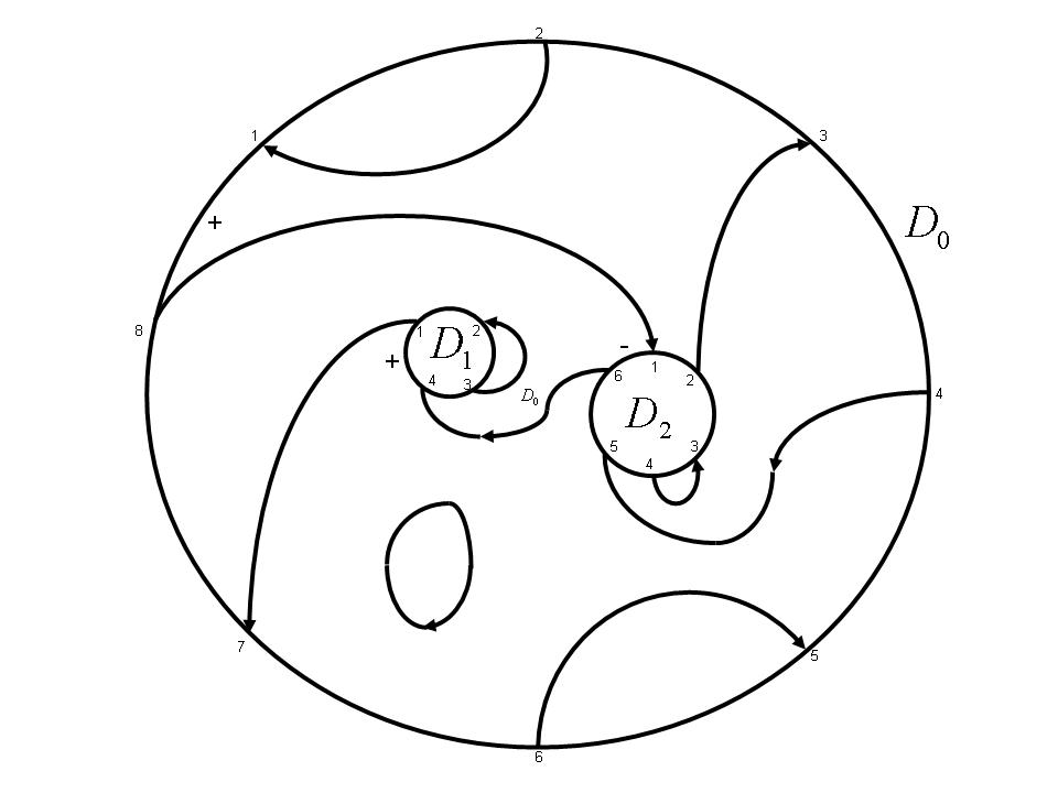
Figure 1. Example of a $(4,+)$-planar tangle with two internal discs $D_{1}$, $D_{2}$ with colours $(2,+)$, $(3,-)$ respectively.

Let $\mathcal{T}((k_{1},\varepsilon_{1}),(k_{2},\varepsilon_{2}),\cdots,(k_{n},\varepsilon_{n});(k,\varepsilon))$ be the set of $(k,\varepsilon)$-planar tangles with $n$ internal discs $D_{1},D_{2},\cdots,D_{n}$ with colours $(k_{1},\varepsilon_{1})$, $(k_{2},\varepsilon_{2})$, $\cdots$, $(k_{n},\varepsilon_{n})$ respectively, $\mathcal{T}(\emptyset;(k,\varepsilon))$ be the set of $(k,\varepsilon)$-planar tangles with no internal disc and $\mathcal{T}_{(k,\varepsilon)}$ be the set of all $(k,\varepsilon)$-planar tangles . The composition of two tangles $T\in\mathcal{T}((k_{1},\varepsilon_{1}),(k_{2},\varepsilon_{2}),\cdots,(k_{n},\varepsilon_{n});(k,\varepsilon))$ and $S\in\mathcal{T}((l_{1},\delta_{1}),(l_{2},\delta_{2}),\cdots,(l_{m},\delta_{m});(k_{i},\varepsilon_{i}))$ (resp. $S\in\mathcal{T}(\emptyset;(k_{i},\varepsilon_{i}))$), denoted by $\left(T\underset{i}{\circ}S\right)\in\mathcal{T}((k_{1},\varepsilon_{1}),\cdots,(k_{i-1},\varepsilon_{i-1}),(l_{1},\delta_{1}),\cdots,(l_{m},\delta_{m}),(k_{i+1},\varepsilon_{i+1}),\cdots,(k_{n},\varepsilon_{n});(k,\varepsilon))$ (resp. $\left(T\underset{i}{\circ}S\right)\in$ $\mathcal{T}((k_{1},\varepsilon_{1}),\cdots,(k_{i-1},\varepsilon_{i-1}),(k_{i+1},\varepsilon_{i+1}),\cdots,(k_{n},\varepsilon_{n});(k,\varepsilon))$), is obtained by gluing the external boundary of $S$ with the boundary of the $i^{\text{th}}$ internal disc of $T$ preserving the marked points on either of them with the help of isotopy, and then erasing the common boundary.

The Planar Tangle Multicategory, denoted by $\mathcal{P}$, is defined as:

• Objects: $\mathcal{P}_{0}=\left\{(k,\varepsilon):k\in\mathbb{N}_{0},\varepsilon\in\{+,-\}\right\}$,

• Morphisms: $\mathcal{P}((k_{1},\varepsilon_{1}),(k_{2},\varepsilon_{2}),\cdots,(k_{n},\varepsilon_{n});(k,\varepsilon))$ (resp. $\mathcal{P}(\emptyset;(k,\varepsilon))$) is the vector space generated by $\mathcal{T}((k_{1},\varepsilon_{1}),(k_{2},\varepsilon_{2}),\cdots,(k_{n},\varepsilon_{n});(k,\varepsilon))$ (resp. $\mathcal{T}(\emptyset;(k,\varepsilon))$) as a basis,

• composition of morphisms is given by the multilinear extension of the composition of tangles as described above,

• the identity morphism $1_{(k,\varepsilon)}\in\mathcal{T}((k,\varepsilon);(k,\varepsilon))\subset\mathcal{P}((k,\varepsilon);(k,\varepsilon))$ is given by the $(k,\varepsilon)$-planar tangle with exactly one internal disc with colour $(k,\varepsilon)$, containing precisely $2k$ strings such that $i^{\text{th}}$ point on the internal disc is connected to the $i^{\text{th}}$ point on the external disc by a string for $1\leq i<2k$.

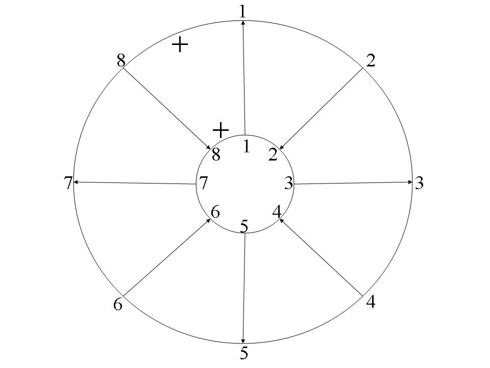
Figure 2. $1_{(4,+)}\in\mathcal{P}((4,\varepsilon);(4,\varepsilon))$

We leave the checking of associativity and identity axioms to the reader. A moment’s observation also reveals that $\mathcal{P}$ is symmetric and has the structure of empty object.

Definition 3.3.

A planar algebra $P$ is a $\mathcal{P}$-algebra, that is, a map of multicategories from $\mathcal{P}$ to $\mathcal{MV}ec$.

Remark 3.4.

The first natural example of planar algebra is the $\mathcal{P}$-algebra which takes the object $(k,\varepsilon)$ to $\mathcal{P}_{(k,\varepsilon)}$, and morphisms $T$ to the multilinear map given by left-compostion of $T$. This is called the Universal Planar Algebra in [Jon2].

Remark 3.5.

For a planar algebra $P$, the collection of vector spaces $\left\{P(k,\varepsilon)\right\}_{k\in\mathbb{N}_{0}}$ forms a unital filtered algebra where $\varepsilon\in\{+,-\}$. The multiplication of $P(k,\varepsilon)$, inclusion of $P(k-1,\varepsilon)$ inside $P(k,\varepsilon)$ and identity of $P(k,\varepsilon)$ are induced by the following tangles:

respectively.

We will now define more structures on a planar algebra. A planar algebra $P$ is said to be connected (resp. locally finite) if $\dim(P(0,+))=1=\dim(P(0,-))$ (resp. $\dim(P(k,\varepsilon))<\infty$ for all $(k,\varepsilon)$). A planar algebra $P$ is said to have modulus $(\delta_{+},\delta_{-})$ if $P(T)=\delta_{+}~{}P(T_{1})$ (resp. $P(T)=\delta_{-}~{}P(T_{1})$) where $T$ is a planar tangle with a contractible loop oriented clockwise (resp. anti-clockwise) and $T_{1}$ is the tangle $T$ with the loop removed. A connected planar algebra $P$ is called spherical if two tangles $T_{1}\in\mathcal{T}_{(0,\varepsilon)}$ and $T_{2}\in\mathcal{T}_{(0,\eta)}$ induce the same multilinear functional by expressing the images of $P(T_{1})$ and $P(T_{2})$ as scalar multiples of the identities of $P(0,\varepsilon)$ and $P(0,\eta)$ respectively whenever one can obtain $T_{1}$ from $T_{2}$ after embedding them on the unit sphere and using spherical isotopy.

Remark 3.6.

If $P=\{P_{n}\}_{n\geq 0}$ is a planar algebra in the sense of Jones ([Jon2]) with modulus $(\delta_{+},\delta_{-})$ (where $Z_{T}$ denotes the action of a tangle $T$ necessarily with positive colors for all discs in it), then one can define a planar algebra $P:\mathcal{P}\rightarrow\mathcal{MV}ec$ via:

(i) $P(k,\varepsilon)=\left\{\begin{array}[]{ll}P_{k}&\text{if }\varepsilon=+\\ Range(Z_{LCE_{k}})&\text{if }\varepsilon=-\end{array}\right.$
where the tangle $LCE_{k}$ is given in Figure 3,

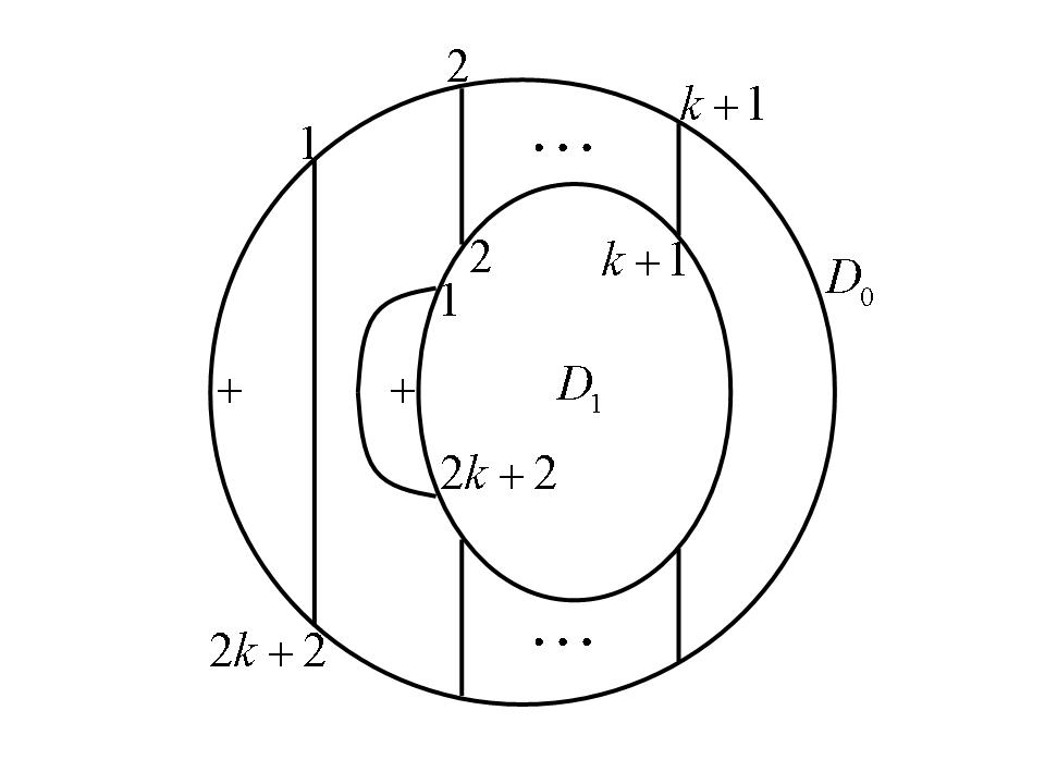
Figure 3. Left conditional expectation tangle

(ii) for $T\in\mathcal{T}((k_{1},\varepsilon_{1}),(k_{2},\varepsilon_{2}),\cdots,(k_{n},\varepsilon_{n});(k_{0},\varepsilon_{0}))$, first define $T^{\prime}=U_{(k_{0},\varepsilon_{0})}\circ T\circ(S_{(k_{1},\varepsilon_{1})},\cdots,S_{(k_{n},\varepsilon_{n})})$ where $S_{(k,+)}=1_{(k,+)}=U_{(k,+)}$, and $S_{(k,-)}$ and $U_{(k,-)}$ are given by the tangles in Figure 4.

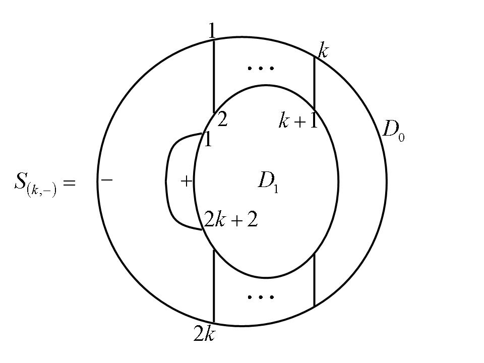
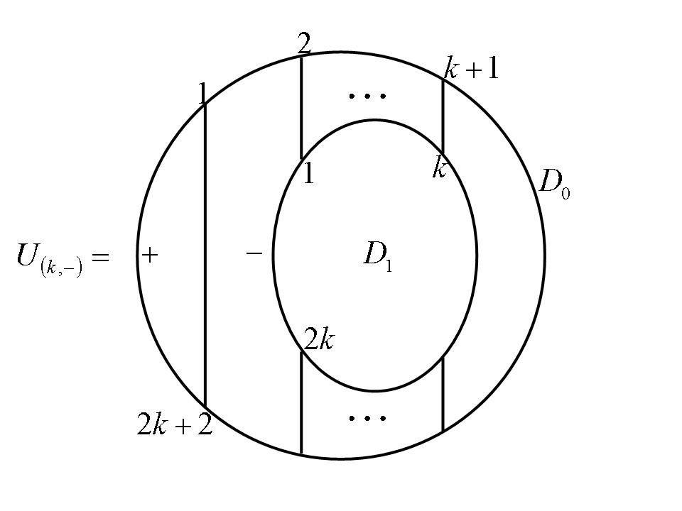
Figure 4.

Note that $T^{\prime}$ is a tangle with positive colors on each of its internal discs. Set $P(T)=\delta_{-}^{-\lvert\{i\geq 1\>:\>\varepsilon_{i}=-\}\rvert}\;Z_{T^{\prime}}|_{P(k_{1},\varepsilon_{1})\times\cdots\times P(k_{n},\varepsilon_{n})}$.

It is routine to check that $P$ preserves composition and identity. The definition of $P$ as a map of multicategories is motivated by Jones’s definition of dual planar algebra (see [Jon2]).

If $T\in\mathcal{T}((k_{1},\varepsilon_{1}),\cdots,(k_{n},\varepsilon_{n});(k,\varepsilon))$ (resp. $T\in\mathcal{T}(\emptyset;(k,\varepsilon))$), then $T^{\ast}\in\mathcal{T}((k_{1},\varepsilon_{1}),\cdots,(k_{n},\varepsilon_{n});(k,\varepsilon))$ (resp. $T^{\ast}\in\mathcal{T}(\emptyset;(k,\varepsilon))$) is defined as the tangle obtained by reflecting $T$ about any straight line not intersecting $T$, and the first point of an internal (resp. external) disc of the reflected $T$ is taken to be the reflected point of the last point of the corresponding internal (resp. external) disc in $T$ such that the reflection preserves the colour of each disc. For example, the $\ast$ of the tangle in Figure 1 is given by the tangle in Figure 5

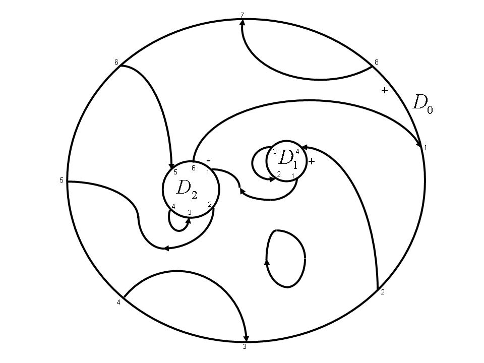
Figure 5.

where we reflect the Figure 1 about a vertical line. We extend the map $\mathcal{T}_{(k,\varepsilon)}\ni T\mapsto T^{\ast}\in\mathcal{T}_{(k,\varepsilon)}$ conjugate linearly to $\ast:\mathcal{P}_{(k,\varepsilon)}\rightarrow\mathcal{P}_{(k,\varepsilon)}$. It is clear that $\ast$ is an involution. This makes $\left\{\mathcal{P}_{(k,\varepsilon)}\right\}_{k\in\mathbb{N}_{0}}$ into a unital filtered $\ast$-algebra for $\varepsilon\in\{+,-\}$. $P$ is said to be a $\ast$ -planar algebra (resp. $C^{\ast}$-planar algebra) if $P$ is a planar algebra, $P(k,\varepsilon)$ is a $\ast$-algebra (resp. $C^{\ast}$-algebra) for each colour $(k,\varepsilon)$ and the map $P$ is $\ast$ preserving in the sense:
if $\theta\in\mathcal{P}((k_{1},\varepsilon_{1}),(k_{2},\varepsilon_{2}),\cdots,(k_{n},\varepsilon_{n});(k,\varepsilon))$ (resp. $\mathcal{P}(\emptyset;(k,\varepsilon))$) and $f_{i}\in P(k_{i},\varepsilon_{i})$ for $1\leq i\leq n$, then $P(\theta^{\ast})(f_{1}^{\ast},\cdots,f_{n}^{\ast})=\left(P(\theta)(f_{1},\cdots,f_{n})\right)^{\ast}$.

A locally finite spherical $C^{\ast}$-planar algebra is called subfactor-planar algebra.

Theorem 3.7.

(Jones) Any extremal subfactor with finite index gives rise to a subfactor-planar algebra. Conversely, any subfactor planar algebra gives rise to an extremal subfactor with finite index.

Jones proved the first part of Theorem 3.7 (in [Jon2]) by prescribing an action of tangles on the standard invariant of a subfactor. However, Jones proved the converse using Popa’s result on $\lambda$-lattices ([Pop2]). Very recently, another proof of the converse using planar algebra techniques appeared in [JSW] and then in [KoSu].

4. Planar Algebra arising from a Bicategory

In this section, we will show how one can construct a planar algebra from a $1$-cell of an abelian ‘pivotal’ strict $2$-category with exactly two $0$- cells. The techniques used in this construction are motivated by Jones’s construction of planar algebra from a subfactor (in [Jon2]).

4.1. Construction of the Planar Algebra

Before we proceed towards the construction, we will first state or deduce some useful results and set up some notations.

Definition 4.1.

A bicategory $\mathcal{B}$ is called pivotal if $\mathcal{B}$ is rigid and there exists a weak transformation $a:id_{\mathcal{B}}\rightarrow\ast\ast$ such that $a_{\varepsilon}=1_{\varepsilon}\in ob(\mathcal{B}(\varepsilon,\varepsilon))$ for all $\varepsilon\in\mathcal{B}_{0}$, where $\ast=(\ast,K)$ is the right dual functor and $\ast\ast=(\ast\ast,J)$ is the weak functor $\ast\circ\ast$.

From now on, we will consider only strict $2$-category instead of general bicategories unless otherwise mentioned; however all results modified with appropriate associativity and unit constraints, will hold even in the absence of the ‘strict’ assumption by the coherence theorem for bicategories.

We next set up some pictorial notation to denote $2$-cells which is analogous to the graphical calculus of morphisms in a tensor category (see [Kas], [BK]). Let $\mathcal{B}$ be a pivotal strict $2$-category as defined above. We denote a $2$-cell $f:Y\rightarrow Z$ by a rectangle labelled with $f$, placed on $\mathbb{R}^{2}$ so that one of the sides is parallel to the $X$-axis and a vertical line segment labelled with $Y$ (resp. $Z$) is attached to the top (resp. bottom) side of the rectangle. Sometimes we will not label the strings attached to a recatangle labelled with a $2$-cell; the $2$-cell itself will induce the obvious labelling to the strings.

We list below pictorial notations of several other $2$-cells which will be the main constituents of the construction without describing them meticulously in words like the way we described $f$ above.

where $Y$, $Z$ are $1$-cells and $f$, $g$ are $2$-cells. To each local maximum or minimum of a string with an orientation marked at the maximum or minimum and labelled with a $1$-cell $Y\in\mathcal{B}(A,B)$, we associate a $2$-cell in the following way:

We will next exhibit some easy consequences in terms of the pictorial notation.

Lemma 4.2.

(i) For any $1$-cell $Y$,

(ii) for any $2$-cell $f:Y\rightarrow Z$, and

(iii) $K_{Y,Z}=$ and $K_{Y,Z}^{-1}=$

(iv) $J_{Y,Z}=$ and $J_{Y,Z}^{-1}=$

(v) $J_{Y,Z}\circ(a_{Y}\otimes a_{Z})=a_{Y\otimes Z}$ for all $1$- cells $Y$ and $Z$.

Proof.

(i) follows from the definition of $Y^{\ast}$ being the right dual of $Y$ and $a$ being invertible.

First part of (ii) follows from the definition of $f^{\ast}$ and naturality of $a$ and the second part easily follows from the first one.

(iii) and (iv) follow from the way the weak functors $\ast$ and $\ast\ast$ are defined.

Definition of the pivotal structure $a$ implies (v). ∎

Remark 4.3.

Parts (iii) and (iv) of the above lemma do not use the pivotal structure $a$ at all. However, with the help of pivotal structure, especially part (v) of the above lemma, one may also prove the following:
$K_{Y,Z}\qquad=$ and $J_{Y,Z}=$

Using the above graphical calculus, we immediately obtain the following relation which will be useful later.

Corollary 4.4.

$a^{-1}_{X^{\ast}}=a^{*}_{X}$ for all $1$-cell $X$.

Proposition 4.5.

For any $2$-cell $f:Y_{1}\otimes\cdots\otimes Y_{n}\rightarrow Z_{1}\otimes\cdots\otimes Z_{m}$, the following identities hold: $=\;f\;=$

Proof.

It is enough to show one of the identities (because applying the reverse rotation and using Lemma 4.2 (i), one can deduce the other identity). We will sketch the proof of the first identity.

For the case $m=n=1$, the result follows trivially from the naturality of $a$.

Suppose $n=2$. Then LHS of the first identity

$=$ $=$

(using Lemma 4.2 (v))
$=$ $=$

(using Lemma 4.2 (i)).

For $n>2$, an analogous result (with $Y_{1}\otimes Y_{2}$ replaced by $Y_{1}\otimes\cdots\otimes Y_{n}$) can be deduced by applying the above result recursively. After working on the rest of the curves (emanating from the top of the rectangle labelled with $f$) in the same way as above, the LHS of the first identity
$=$

$=a_{Z_{1}\otimes\cdots\otimes Z_{m}}^{-1}\circ f^{\ast\ast}\circ a_{Y_{1}\otimes\cdots\otimes Y_{n}}=f$ (using naturality of $a$). ∎

We now construct a planar algebra from a bicategory. Let $\mathcal{B}$ be a pivotal $\mathbb{C}$-linear strict $2$-category with $\{+,-\}$ as the set of $0$-cells and fix $X\in ob(\mathcal{B}(-,+))$. For each colour $(k,\varepsilon)$, set

$$X_{(k,\varepsilon)}$$

if $k\geq 1$ and $X_{(0,\varepsilon)}=1_{\varepsilon}\in ob(\mathcal{B}(\varepsilon,\varepsilon))$. Define $P_{(k,\varepsilon)}=End(X_{(k,\varepsilon)})$.

Now, for a $(k,\varepsilon)$-planar tangle $\theta\in\mathcal{T(}(k_{1},\varepsilon_{1}),(k_{2},\varepsilon_{2}),\cdots,(k_{n},\varepsilon_{n});(k,\varepsilon)),$ we wish to define a multilinear map $P(\theta):P_{(k_{1},\varepsilon_{1})}\times\cdots\times P_{(k_{n},\varepsilon_{n})}\rightarrow P_{(k,\varepsilon)}$. For this we extensively use the graphical calculus of the $2$-cells of $\mathcal{B}$.

For the ease of dealing with $2$-cells replaced by labelled rectangles, we will consider the planar tangle $\theta$ as an isotopy class of pictures where each disc (internal or external) is replaced by a rectangle with first half of the strings being attached to one of the side (called the top side) and the remaining half of the strings attached to the opposite side (called the bottom side). Next, in the isotopy class of $\theta$, we fix a picture $\Theta$ placed on $\mathbb{R}^{2}$ with the bottom side of the external rectangle being parallel to the $X$-axis, satisfying the following properties:

• the collection of strings in $\Theta$ must have finitely many local maximas and minimas,

• each internal rectangle is aligned in such a way that the top side of the external rectangle is parallel and also nearer to the top side of the internal rectangle than its bottom side,

• the projections of the maxima, minima and one of the vertical sides of each internal rectangle (that is, the sides other than the top and bottom ones) on the vertical sides of the external rectangle of $\Theta$ are disjoint.

We will say that an element $\Theta$ in the isotopy class of $\theta$ is in standard form if $\Theta$ satisfies the above conditions. For example, a standard form representation of the tangle in Figure 1 will be the following diagram

Let $\Theta$ be an element in standard form of the isotopy class of $\theta$. We now cut $\Theta$ into horizontal stripes so that every stripe should have at most one local maxima, minima or internal rectangle. Each component of every string in a horizontal stripe is labelled with $X$ or $X^{\ast}$ according as the orientation of the string is from the bottom side to the top side of the horizontal stripe or reverse respectively; each local maxima or minima is labelled with $X$ and the orientation is induced by the orientation of the actual string in $\Theta$. For example,
will be replaced by

To define $P(\theta):P_{(k_{1},\varepsilon_{1})}\times\cdots\times P_{(k_{n},\varepsilon_{n})}\rightarrow P_{(k,\varepsilon)}$, we fix $2$-cells $f_{i}\in P_{(k,\varepsilon)}$ for $1\leq i\leq n$. We label the $i^{\text{th}}$ internal rectangle (contained in some horizontal stripe) with $f_{i}$. Now, each horizontal stripe makes sense as a $2$-cell according to the notation already set up. We define $P(\theta)(f_{1},f_{2},\cdots,f_{n})$ as the composition of these $2$-cells. It is easy to easy that $P(\theta)$ is a multilinear map from $P_{(k_{1},\varepsilon_{1})}\times\cdots\times P_{(k_{n},\varepsilon_{n})}$ to $P_{(k,\varepsilon)}$. Natural question to ask will be why $P(\theta)(f_{1},f_{2},\cdots,f_{n})$ is independent of the choice of $\Theta$ in the isotopy class of $\theta$.

For this, first note that one standard form representative of a tangle can be obtained from another applying finitely many moves of the following three types:

(i) Sliding Move: $\sim$

(ii) Rotation Move:

(iii) Wiggling Move:

where $f$ and $g$ are $2$-cells. To show $P(\theta)(f_{1},f_{2},\cdots,f_{n})$ is well-defined, it is enough to show that two standard form representatives $\Theta_{1}$ and $\Theta_{2}$ of $\theta$ labelled with $\{f_{1},f_{2},\cdots,f_{n}\}$, differing by any of the above three moves, will assign identical $2$-cell. Invariance under sliding moves hold from the functoriality of $\otimes$ and rotation moves follow from Proposition 4.5 and Corollary 4.4; finally, wiggling moves are justified by Lemma 4.2 (i). Thus, we have a well-defined map $P:\mathcal{T}((k_{1},\varepsilon_{1}),\cdots,(k_{n},\varepsilon_{n});(k,\varepsilon))\rightarrow\mathcal{MV}ec((P_{(k_{1},\varepsilon_{1})},\cdots,P_{(k_{n},\varepsilon_{n})};P_{(k,\varepsilon)})$ (resp. $P:\mathcal{T}(\emptyset;(k,\varepsilon))\rightarrow\mathcal{MV}ec(\emptyset;P_{(k,\varepsilon)})$). Finally, define the planar algebra $P:\mathcal{P\rightarrow MV}ec$ via:

• $P(k,\varepsilon)=P_{(k,\varepsilon)}$,

• the linear map $P:\mathcal{P}((k_{1},\varepsilon_{1}),\cdots,(k_{n},\varepsilon_{n});(k,\varepsilon))\rightarrow\mathcal{MV}ec(P_{(k_{1},\varepsilon_{1})},\cdots,P_{(k_{n},\varepsilon_{n})};P_{(k,\varepsilon)})$ (resp. $P:\mathcal{P}(\emptyset;(k,\varepsilon))\rightarrow\mathcal{MV}ec(\emptyset;P_{(k,\varepsilon)})$) is defined by extending the map $P:\mathcal{T}((k_{1},\varepsilon_{1}),\cdots,(k_{n},\varepsilon_{n});(k,\varepsilon))\rightarrow\mathcal{MV}ec(P_{(k_{1},\varepsilon_{1})},\cdots,P_{(k_{n},\varepsilon_{n})};P_{(k,\varepsilon)})$ (resp. $P:\mathcal{T}(\emptyset;(k,\varepsilon))\rightarrow\mathcal{MV}ec(\emptyset;P_{(k,\varepsilon)})$) linearly.

Clearly, $P(1_{(k,\varepsilon)})=id_{P((k,\varepsilon))}$ for all $(k,\varepsilon)$. To check $P$ preserves composition of morphisms, let us consider two tangles $T$ and $S$ such that the first internal disc $D_{1}$ of $T$ has color $(k,\varepsilon)$ same as that of $S$. Choose $T_{1}$ and $S_{1}$ as standard form representatives of $T$ and $S$ respectively such that dimension of the external disc of $S_{1}$ along with the marked points match with that of $D_{1}$ in $T_{1}$. Let $T_{1}\underset{D_{1}}{\circ}S_{1}$ denote the picture obtained by replacing $D_{1}$ by $S_{1}$ and then erasing the external boundary of $S_{1}$. Note that $T_{1}\underset{D_{1}}{\circ}S_{1}$ is a standard form representative of $T\underset{D_{1}}{\circ}S$. Now, we consider $2$-cells for each internal discs (except $D$) in $T$ and $S$ coming from the appropriate vector spaces and label the corresponding rectangles in $T_{1}$, $S_{1}$, and $T_{1}\underset{D_{1}}{\circ}S_{1}$ with them. If we slice $T_{1}\underset{D_{1}}{\circ}S_{1}$ as described while defining the action of $P$ on the morphism spaces and induce the slicing of $T_{1}\underset{D_{1}}{\circ}S_{1}$ on $T_{1}$ and $S_{1}$, then the $2$-cells corresponding to the slices appearing in $T_{1}\underset{D_{1}}{\circ}S_{1}$ are the same as those for $T_{1}$ with the slice containing $D_{1}$ being replaced by the slices coming from $S_{1}$. Thus $P$ must preserve composition.

This completes the construction of the planar algebra.

5. Affine Representations of a Planar Algebra

In this section, we will introduce the notion of an affine representation of a planar algebra which is a generalization of the concept of the Hilbert space representation of annular Temperley-Lieb by Vaughan Jones and Sarah Reznikoff ([JR]); one can also treat this as an annular representations of a planar algebra with rigid boundaries. We then discuss some general theory of the affine representations following exactly the way Jones developed the theory for annular representations in [Jon3].

Before going into the definition of affine representations, we will first introduce the affine category over a planar algebra.

Definition 5.1.

An $((m,\eta),(n,\varepsilon))$-affine tangle is an isotopy class of pictures consisting of:

• the annulus $\mathcal{A}=\{z\in\mathbb{C}:1\leq z\leq 2\}$,

• the set of points $\{2e^{-\frac{k\pi i}{m}}:0\leq k\leq 2m-1\}$ (resp. $\{e^{-\frac{k\pi i}{n}}:0\leq k\leq 2n-1\}$) are numbered clockwise starting from $2$ (resp. $1$) as the first points,

• $\mathcal{A}$ consists of internal discs $D_{1}$, $D_{2}$,$\cdots$, $D_{l}$ with colour $(k_{1},\varepsilon_{1})$, $(k_{2},\varepsilon_{2})$,$\cdots$,$(k_{l},\varepsilon_{l})$ respectively and non-intersecting oriented strings (just like in an ordinary planar tangle described in Definition 3.1) so that the inner (resp. outer) boundary of $\mathcal{A}$ gets the colour $\left(n,\varepsilon\right)$ (resp. $\left(m,\eta\right)$),

• any isotopy should keep the boundary of $\mathcal{A}$ fixed.

Figure 6. Example of a $\left(\left(2,-\right),\left(1,+\right)\right)$-affine tangle

Let $P$ be a planar algebra. An $((m,\eta),(n,\varepsilon))$-affine tangle is said to be $P$-labelled if, to each internal disc $D$ of $\mathcal{A}$ with colour $(k,\varepsilon^{\prime})$, an element of $P_{(k,\varepsilon^{\prime})}$ is assigned. Let $\mathcal{A}_{(n,\varepsilon)}^{(m,\eta)}$ denote the set of all $((m,\eta),(n,\varepsilon))$-affine tangles and $\mathcal{A}_{(n,\varepsilon)}^{(m,\eta)}(P)$ denote the set of all $P$-labelled $((m,\eta),(n,\varepsilon))$-affine tangles. If $A\in\mathcal{A}_{(n,\varepsilon)}^{(m,\eta)}$ and $B\in\mathcal{A}_{(l,\delta)}^{(n,\varepsilon)},$ then we can define $A\circ B$ ($\in\mathcal{A}_{(l,\delta)}^{(m,\eta)}$) as the affine tangle obtained by considering the picture $\frac{1}{2}(2A\cup B)$. We might have to smoothen out the strings which are attached with the inner boundary of $2A$ and outer boundary of $B$; this can also be avoided by requiring the strings to meet the inner and the outer boundaries radially in the definition of an affine tangle.

We now set up a convenient way of sketching an affine tangle; instead of marking the points on the inner (resp. outer) boundary at the roots of unity (resp. twice the roots of unity), we will mark them close to each other on the top with $1$ as the leftmost point. Further, with the help of isotopy, every $A\in\mathcal{A}_{(n,\varepsilon)}^{(m,\eta)}$ can be expressed as:

for some $T\in\mathcal{T}_{(m+n+l,\eta)}$. Note that $T$ and $l$ are not unique. For example, the affine tangle in Figure 6 can be expressed as the above annular tangle for $m=2$, $n=1$, $l=1$ and $T\;=$

and $\eta=-$.

Let $(F\mathcal{A}P)_{(n,\varepsilon)}^{(m,\eta)}$ be the vector space with $\mathcal{A}_{(n,\varepsilon)}^{(m,\eta)}(P)$ as a basis, $\mathcal{T}_{(k,\varepsilon)}(P)$ be the set of all $P$-labelled $(k,\varepsilon)$-planar tangles, $\mathcal{P}_{(k,\varepsilon)}$ (resp. $\mathcal{P}_{(k,\varepsilon)}(P)$) be the vector space with $\mathcal{T}_{(k,\varepsilon)}$ (resp. $\mathcal{T}_{(k,\varepsilon)}(P)$) as a basis and $\Psi_{(m,\eta),(n,\varepsilon)}^{l}$ be the annular tangle .

Observe that $\Psi_{(m,\eta),(n,\varepsilon)}^{l}$ induces a linear map $\psi_{(m,\eta),(n,\varepsilon)}^{l}:\mathcal{P}_{(m+n+l,\eta)}\rightarrow(F\mathcal{A}P)_{(n,\varepsilon)}^{(m,\eta)}$ which also lifts to the level of the $P$-labelled ones. Moreover, for any $A\in(F\mathcal{A}P)_{(n,\varepsilon)}^{(m,\eta)}$, there exists $l\in\mathbb{N}_{0}$ and $T\in\mathcal{P}_{(m+n+l,\eta)}(P)$ such that $A=\psi_{(m,\eta),(n,\varepsilon)}^{l}(T)$. Set

$$\mathcal{W}_{(n,\varepsilon)}^{(m,\eta)}=\left\{A\in(F\mathcal{A}P)_{(n,\varepsilon)}^{(m,\eta)}\left|\begin{array}[]{c}A=\psi_{(m,\eta),(n,\varepsilon)}^{l}(T)\text{ for some }l\in\mathbb{N}_{0}\text{, }T\in\mathcal{P}_{(m+n+l,\eta)}(P)\\ \text{such that }P(T)=0\in P(m+n+l,\eta)\end{array}\right.\right\}\text{.}$$

where we use the linear map $P:\mathcal{P}_{(k,\varepsilon)}(P)\rightarrow P(k,\varepsilon)$ induced by the map of multicategories $P$. It is a fact that $\mathcal{W}_{(n,\varepsilon)}^{(m,\eta)}$ is a vector subspace of $(F\mathcal{A}P)_{(n,\varepsilon)}^{(m,\eta)}$. For instance, if $A_{i}\in\mathcal{W}_{(n,\varepsilon)}^{(m,\eta)}$ and $l_{i}\in\mathbb{N}_{0}$, $T_{i}\in\mathcal{P}_{(m+n+l_{i},\eta)}(P)$ such that $A_{i}=\psi_{(m,\eta),(n,\varepsilon)}^{l_{i}}(T_{i})$, $P(T_{i})=0$ for $i=1$, $2$ and $l_{1}\leq l_{2}$, then one can obtain $\widetilde{T_{1}}\in\mathcal{P}_{(m+n+l_{2},\eta)}(P)$ such that $A_{1}=\psi_{(m,\eta),(n,\varepsilon)}^{l_{2}}(\widetilde{T_{1}})$ by wiggling back and forth a string emanating from either of the vertical sides of $T_{1}$ around the inner disc of $A_{1}$ until the total number of strings around the inner disc of $A_{1}$ increases from $l_{1}$ to $l_{2}$; finally, $A_{1}+A_{2}=\psi_{(m,\eta),(n,\varepsilon)}^{l_{2}}(\widetilde{T_{1}}+T_{2})$.

Define the category $\mathcal{A}ffP$ by:

• $ob(\mathcal{A}ffP)=\{(k,\varepsilon):k\in\mathbb{N}_{0},\varepsilon\in\{+,-\}\}$

• $Hom_{(\mathcal{A}ffP)}((n,\varepsilon),(m,\eta))=\frac{(F\mathcal{A}P)_{(n,\varepsilon)}^{(m,\eta)}}{\mathcal{W}_{(n,\varepsilon)}^{(m,\eta)}}=$ the quotient vector space of $(F\mathcal{A}P)_{(n,\varepsilon)}^{(m,\eta)}$ over $\mathcal{W}_{(n,\varepsilon)}^{(m,\eta)}$ (also denoted by $\left(\mathcal{A}ffP\right)_{(n,\varepsilon)}^{(m,\eta)}$),

• the composition of affine tangles is linearly extended for $(F\mathcal{A}P)$’s; one can easily verify that $A\circ B$ $\in\mathcal{W}_{(l,\delta)}^{(m,\eta)}$ whenever $A\in\mathcal{W}_{(n,\varepsilon)}^{(m,\eta)}$ and $B\in(F\mathcal{A}P)_{(l,\delta)}^{(n,\varepsilon)}$, or $A\in(F\mathcal{A}P)_{(l,\delta)}^{(n,\varepsilon)}$ and $B\in\mathcal{W}_{(n,\varepsilon)}^{(m,\eta)}$; this implies the composition is induced in the level of quotient vector spaces as well,

• the identity of $(k,\varepsilon)$ denoted by $1_{(k,\varepsilon)}$, is given by an $((k,\varepsilon),(k,\varepsilon))$-affine tangle obtained by joining the $i^{\text{th}}$ point of the inner boundary with the $i^{\text{th}}$ point of the outer boundary by a straight string for all $i$.

We will refer the category $\mathcal{A}ffP$ as affine category over $P$.

Definition 5.2.

An additive functor $F:\mathcal{A}ffP\rightarrow\mathcal{V}ec$ is said to be an affine representation of $P$.

Remark 5.3.

The functor induced by $P$ itself gives an affine representation of $P$; this is called the ‘trivial’ affine representation.

Lemma 5.4.

If $F$ is an affine representation of $P,$ then

(a) $F(k,\varepsilon)\hookrightarrow F(k+1,\varepsilon)$,

(b) $F(k,\varepsilon)$ is isomorphic to $F(k,-\varepsilon)$
for all colours $(k,\varepsilon)$.

Proof.

The inclusion in part (a) is given by considering the $F$-image of the inclusion tangle.

For part (b), consider the rotation tangle $R_{(k,\varepsilon)}\in\mathcal{A}_{(k,\varepsilon)}^{(k,-\varepsilon)}$ obtained by joining the points $e^{-\frac{l\pi i}{k}}$ and $2e^{-\frac{(l+1)\pi i}{k}}$ on the boundary of $\mathcal{A}$ by a string which does not make a full round about the inner disc. $F(R_{(k,\varepsilon)})$ gives the desired isomorphism in (b) ∎

Remark 5.5.

It may seem so that $\left(R_{(k,\varepsilon)}\right)^{2k}$ is the identity $((k,\varepsilon),(k,\varepsilon))$-affine tangle (that is, the tangle obtained by joining the points $e^{-\frac{l\pi i}{k}}$ and $2e^{-\frac{l\pi i}{k}}$ by a straight line), but this is not true because of the restriction of the isotopy being identity on boundary of $\mathcal{A}$. This is the main difference between the annular representations of $P$ (in [Jon3] and [Gho]) and the affine representations.

The weight of an affine representation $F$ denoted by $wt(F)$, is given by the smallest integer $k$ such that $\dim(F(k,\varepsilon))\neq\{0\}$. The $wt(F)$ is well-defined by Lemma 5.4.

An affine representation $F$ will be called locally finite if $F(k,\varepsilon)$ is finite dimensional for all colours $(k,\varepsilon)$. The dimension of an affine representation $F$ is defined as a pair of formal power series $(\Phi_{F}^{+},\Phi_{F}^{-})$ where

$$\Phi_{F}^{\varepsilon}(z)=\sum_{k=0}^{\infty}\dim(F(k,\varepsilon))~{}z^{k}~{}~{}~{}~{}\text{ for }\varepsilon\in\{+,-\}\text{.}$$

Question: If $P$ is a planar algebra with modulus $(\delta,\delta)$, is the radius of convergence of the dimension of an affine representation greater than or equal to $\delta^{-2}$?

The above question appeared in [Jon3] for annular representations of a planar algebra. The question for annular representations was answered in affirmative for the Temperley-Lieb planar algebras by Jones (in [Jon3]) and for the Group Planar Algebras by Ghosh (in [Gho]). We will show the same for affine representations of any finite depth planar algebra in the Section 6.

Let $P$ be a $\ast$- or a $C^{\ast}$-planar algebra. Then, $\mathcal{P}_{(k,\varepsilon)}(P)$ becomes a $\ast$-algebra where $\ast$ of a labelled tangle is given by $\ast$ of the unlabelled tangle whose internal discs are labelled with $\ast$ of the labels. One can define $\ast$ of an affine tangle by relecting it around a circle concentric to inner or outer boundary and then isotopically stretch or shirnk to fit into the annulus $\mathcal{A}$ such that the first point of inner or outer boundary after reflection remains the same whereas the first point of any internal disc after reflection is given by the reflection of the last point and colours of all discs are preserved; this can be induced in the $P$-labelled ones by labelling the internals discs of the reflected tangle with $\ast$ of the labels. Note that $\ast$ is an involution. Extending $\ast$ conjugate linearly, we can define the map $\ast:\left(F\mathcal{A}P\right)_{(n,\varepsilon)}^{(m,\eta)}\rightarrow\left(F\mathcal{A}P\right)_{(m,\eta)}^{(n,\varepsilon)}$ for all colours $(m,\eta)$, $(n,\varepsilon)$. It is easy to check that $\ast\left(\mathcal{W}_{(n,\varepsilon)}^{(m,\eta)}\right)=\mathcal{W}_{(m,\eta)}^{(n,\varepsilon)}$. This makes the category $\mathcal{A}ffP$ a $\ast$-category. An additive functor $F:\mathcal{A}ffP\rightarrow\mathcal{H}il$ is said to be an affine $\ast$-representation if $F$ is $\ast$ preserving, that is, $F\left(A^{\ast}\right)=\left(F(A)\right)^{\ast}$ for all $A\in Mor_{\mathcal{A}ffP}$ where $\mathcal{H}il$ denotes the category of Hilbert spaces.

Remark 5.6.

Note that if $F$ is an affine $\ast$-representation, then $\langle F(A)(v),w\rangle=\langle v,F(A^{\ast})(w)\rangle$ for all $A\in\left(\mathcal{A}ffP\right)_{(n,\varepsilon)}^{(m,\eta)}$, $v\in F(n,\varepsilon)$, $w\in F(m,\eta)$.

The category of affine representations of a planar algebra $P$ with natural transformations as morphism space, forms an abelian category and the dimension is additive with respect to direct sum. One can further talk about irreducibilty and indecomposability of an affine representation (see [Jon3] for details). For example, the trivial affine representation of $P$ is irreducible. However, if we restrict ourselves to the case of a locally finite, non-degenerate $C^{\ast}$-planar algebra $P$ and the category of locally finite affine $\ast$-representations, the notions of irreducibility and indecomposability coincide. In this case, one can also talk about orthogonality of affine representations. These treatments for annular representations can be found in more details in [Jon3].

Jones indicated a procedure of finding annular representations of a locally finite $C^{\ast}$-planar algebra $P$ with modulus $(\delta,\delta)$ in [Jon3]; the same works for the affine ones as well. For this, we need to consider a subspace of the morphism space $\left(\mathcal{A}ffP\right)_{(k,\varepsilon)}^{(k,\varepsilon)}$, namely,

$$\left(\widehat{\mathcal{A}ffP}\right)_{(k,\varepsilon)}=\left\{A\in\left(\mathcal{A}ffP\right)_{(k,\varepsilon)}^{(k,\varepsilon)}\left|\begin{tabular}[]{c}$A\text{ is a linear combination of}$\\ $\text{elements of the form }B\circ C\text{ where}$\\ $B\in\left(\mathcal{A}ffP\right)_{(n,\eta)}^{(k,\varepsilon)}\text{, }C\in\left(\mathcal{A}ffP\right)_{(k,\varepsilon)}^{(n,\eta)}$\\ $\text{for some colour }(n,\eta)\text{ such that }n<k$\end{tabular}\right.\right\}\text{.}$$

It is easy to see that $\left(\widehat{\mathcal{A}ffP}\right)_{(k,\varepsilon)}$ is an ideal in $\left(\mathcal{A}ffP\right)_{(k,\varepsilon)}^{(k,\varepsilon)}$. We list some common properties shared by affine $\ast$-representations and annular $\ast$-representations of $P$; the proofs can be found in [Jon3].

(i) An affine representation $F$ is irreducible iff $F(k,\varepsilon)$ is irreducible as an $\left(\mathcal{A}ffP\right)_{(k,\varepsilon)}^{(k,\varepsilon)}$-module for all colours $\left(k,\varepsilon\right)$.

(ii) If $W$ is an irreducible $\left(\mathcal{A}ffP\right)_{(k,\varepsilon)}^{(k,\varepsilon)}$-submodule of $F(k,\varepsilon)$ for some colour $\left(k,\varepsilon\right)$, then $W$ generates an irreducible subrepresentation of $F$.

(iii) Orthogonal $\left(\mathcal{A}ffP\right)_{(k,\varepsilon)}^{(k,\varepsilon)}$-submodules of $F(k,\varepsilon)$ for some colour $\left(k,\varepsilon\right)$, generate orthogonal subrepresentations of $F$.

(iv) If $F$ and $G$ are representations with $F$ being irreducible and if $\theta:F(k,\varepsilon)\rightarrow G(k,\varepsilon)$ is a non-zero $\left(\mathcal{A}ffP\right)_{(k,\varepsilon)}^{(k,\varepsilon)}$-linear homomorphism for some colour $\left(k,\varepsilon\right)$, then $\theta$ extends to an injective homomorphism from $\ F$ to $G$, that is, an injective natural transformation from $F$ to $G$.

(v) If $W_{\left(k,\varepsilon\right)}=$ $span\{F(A)\left(v\right):A\in\left(\mathcal{A}ffP\right)_{(n,\eta)}^{(k,\varepsilon)},v\in F(n,\eta),k>n\geq 0\}\subset F{\left(k,\varepsilon\right)}$, then

$$\left(W_{\left(k,\varepsilon\right)}\right)^{\perp}=\bigcap_{A\in\left(\widehat{\mathcal{A}ffP}\right)_{(k,\varepsilon)}}kernel(F(A))\text{.}$$

From (v), we can conclude that for an affine $\ast$-representation $F$ with weight $k$, we have

$$F(k,\varepsilon)=\bigcap_{A\in\left(\widehat{\mathcal{A}ffP}\right)_{(k,\varepsilon)}}kernel(F(A))$$

since $W_{\left(k,\varepsilon\right)}$ turns out to be zero and hence $F(k,\varepsilon)$ forms a module over the quotient $\frac{\left(\mathcal{A}ffP\right)_{(k,\varepsilon)}^{(k,\varepsilon)}}{\left(\widehat{\mathcal{A}ffP}\right)_{(k,\varepsilon)}}$. We denote this quotient algebra by $\left(LWP\right)_{(k,\varepsilon)}$ (Lowest Weight algebra at $(k,\varepsilon)$).

By (i), if F is an irreducible affine $\ast$-representation with weight $k$, then $F(k,\varepsilon)$ is an irreducible module over $(LWP)_{(k,\varepsilon)}$. In order to find the irreducible affine $\ast$-representations of $P$, it suffices to do the following:

(i) find the irreducible representations of $(LWP)_{(k,\varepsilon)}$,

(ii) find which irreducible representation of $(LWP)_{(k,\varepsilon)}$ gives rise to an irreducible affine $\ast$-representation of the planar algebra.

We will use this method to deduce some results on the irreducible affine $\ast$-representations of a finite depth planar algebra in the next section.

6. Finite Depth Planar Algebras

In this section, we will recall the notion of the depth of a planar algebra which is motivated from the depth of a finite index subfactor. We then prove some finiteness results for the category of affine representation of subfactor-planar algebras. Finally, we answer the question mentioned in Section 5 for subfactor-planar algebras with finite depth.

Let $P$ be a planar algebra with modulus $(\delta_{+},\delta_{-})$. We first define below a tangle called Jones projections.
$E_{(k,\varepsilon)}=P\left(\includegraphics[scale={0.16},bb=0250700550]{pictures/fdpa/E_k.jpg}\right)\in P_{(k+1,\varepsilon)}$ where $k\in\mathbb{N}$ and $\varepsilon\in\left\{+,-\right\}$.
Note that $E_{(k,\varepsilon)}^{2}=\left\{\begin{array}[]{ll}\delta_{\varepsilon}E_{(k,\varepsilon)}&\text{if }k\text{ is odd}\\ \delta_{-\varepsilon}E_{(k,\varepsilon)}&\text{if }k\text{ is even}\end{array}\right.$

From now on, we will work with the case $\delta_{+}=\delta_{-}=\delta$. In this case, $e_{(k,\varepsilon)}=\frac{1}{\delta}~{}E_{(k,\varepsilon)}$ becomes an idempotent. Two more immediate consequences are:

(i) $E_{(k,\varepsilon)}\cdot E_{(k\pm 1,\varepsilon)}\cdot E_{(k,\varepsilon)}=E_{(k,\varepsilon)}$,

(ii) $E_{(k,\varepsilon)}\cdot E_{(l,\varepsilon)}=E_{(l,\varepsilon)}\cdot E_{(k,\varepsilon)}$ whenever $\left|k-l\right|\geq 2$

where $\cdot$ denotes the multiplication in the planar algebra $P$.

Lemma 6.1.

The subspace $I_{(k,\varepsilon)}=P_{(k,\varepsilon)}e_{(k,\varepsilon)}P_{(k,\varepsilon)}=span\left\{x\cdot e_{(k,\varepsilon)}\cdot y:x,y\in P_{(k,\varepsilon)}\right\}$ is a two-sided ideal of $P_{(k+1,\varepsilon)}$.

Proof.

The proof of being right ideal easily follows by considering the tangle

and noting that the range of the $P$ action of this tangles is inside $I_{(k,\varepsilon)}$. Proof of left ideal follows from the same tangle with upside down. ∎

Lemma 6.2.

If $I_{(k,\varepsilon)}=P_{(k+1,\varepsilon)}$, then $I_{(k+1,\varepsilon)}=P_{(k+2,\varepsilon)}$.

Proof.

By Lemma 6.1, $I_{(k+1,\varepsilon)}$ is an ideal in $P_{(k+2,\varepsilon)}$. So, it is enough to show $1\in I_{(k+1,\varepsilon)}$. Now, implies $1\in P_{(k+1,\varepsilon)}=I_{(k,\varepsilon)}=P_{(k,\varepsilon)}E_{(k,\varepsilon)}P_{(k,\varepsilon)}=P_{(k,\varepsilon)}E_{(k,\varepsilon)}E_{(k+1,\varepsilon)}E_{(k,\varepsilon)}P_{(k,\varepsilon)}\subset P_{(k+1,\varepsilon)}E_{(k,\varepsilon)}P_{(k+1,\varepsilon)}=I_{(k+1,\varepsilon)}$. ∎

Lemma 6.3.

If $I_{(k,\varepsilon)}=P_{(k+1,\varepsilon)}$, then $\left\{\begin{array}[]{ll}I_{(k,-\varepsilon)}=P_{(k+1,-\varepsilon)}&\text{if }k\text{ is even}\\ I_{(k+1,-\varepsilon)}=P_{(k+2,-\varepsilon)}&\text{if }k\text{ is odd.}\end{array}\right.$

Proof.

Consider the tangles $S_{(k,\varepsilon)}=$ $\in\mathcal{T}\left((k,\varepsilon),(k,\varepsilon);(k+1,\varepsilon)\right)$

and $R_{k}=$ $\in\mathcal{T}\left((k,\varepsilon);(k,-\varepsilon)\right)$

where $R_{k}$ of course depends on the $\varepsilon$ which will be automatically determined from the context. Note that $I_{(k,\varepsilon)}=P_{(k+1,\varepsilon)}$ if and only if $P_{(k+1,\varepsilon)}=Range\left(P\left(S_{(k,\varepsilon)}\right)\right)$ ($=$ span of the image of $P\left(S_{(k,\varepsilon)}\right)$).

We first consider the case $k$ being even. Then, isotopically $\left(R_{k+1}\right)^{k+1}\circ S_{(k,\varepsilon)}\circ\left(\left(R_{k}\right)^{k+1},\left(R_{k}\right)^{k-1}\right)=S_{(k,-\varepsilon)}$. Hitting both sides with $P$ and using the invertibility of the rotation tangles, we get the desired equality.

If $k$ is odd, then by Lemma 6.1, $I_{(k+1,\varepsilon)}=P_{(k+2,\varepsilon)}$ where $k+1$ is even and thus we are through by the first case. ∎

Remark 6.4.

Note that in the above three lemmas, the modulus of $P$ is not used at all.

Definition 6.5.

A planar algebra $P$ is said to have finite depth if $I_{(l,\varepsilon)}=P_{(l+1,\varepsilon)}$ for some $l\in\mathbb{N}$, $\varepsilon\in\left\{+,-\right\}$ and in that case, the depth of $P$ will be a pair of natural numbers $\left(l_{+},l_{-}\right)$ such that $l_{\varepsilon}$ is the smallest natural number such that $I_{(l_{\varepsilon},\varepsilon)}=P_{(l_{\varepsilon}+1,\varepsilon)}$.

Remark 6.6.

From Lemma 6.3, one can deduce that if $\left(l_{+},l_{-}\right)$ denotes the depth of $P$ and $l_{\varepsilon}$ is even (resp. odd), then $l_{-\varepsilon}\in\left\{l_{\varepsilon}-1,l_{\varepsilon}\right\}$ (resp. $l_{-\varepsilon}\in\left\{l_{\varepsilon},l_{\varepsilon}+1\right\}$), that is, either both $l_{+}$ and $l_{-}$ are same or they are consecutive natural numbers with the larger one being even.

Let $S_{\left(k,\varepsilon\right)}^{(m)}$ denote the tangle $\in\mathcal{T}_{(k+m-1,\varepsilon)}$.

Note that $S_{\left(k,\varepsilon\right)}^{(1)}=1_{\left(k,\varepsilon\right)}$ and $S_{\left(k,\varepsilon\right)}^{(2)}=S_{\left(k,\varepsilon\right)}$ (defined in the proof of the Lemma 6.3).

Lemma 6.7.

If $P$ has finite depth with depth $\left(l_{+},l_{-}\right)$, then

$$Range\left\{P\left(S_{\left(k,\varepsilon\right)}^{(m)}\right)\right\}=P\left(k+m-1,\varepsilon\right)$$

whenever $k\geq l_{\varepsilon}=$ the $\varepsilon$-depth of $P$ and $m\in\mathbb{N}$.

Proof.

The case $m=1$ is trivial and $m=2$ follows from the proof of Lemma 6.3.

Suppose the statement of the lemma is true for all $m\leq n$. To show the same for $m=\left(n+1\right)$, we consider the tangle $S_{\left(k+n-1,\varepsilon\right)}^{(2)}\circ\left(S_{\left(k,\varepsilon\right)}^{(n)},S_{\left(k,\varepsilon\right)}^{(n)}\right)$. Clearly,

$$Range\left(P\left(S_{\left(k+n-1,\varepsilon\right)}^{(2)}\circ\left(S_{\left(k,\varepsilon\right)}^{(n)},S_{\left(k,\varepsilon\right)}^{(n)}\right)\right)\right)=P\left(k+n,\varepsilon\right)$$

since $k\geq l_{\varepsilon}$. Again, for even $n$ ($=2p$ say), the tangle $S_{\left(k+n-1,\varepsilon\right)}^{(2)}\circ\left(S_{\left(k,\varepsilon\right)}^{(n)},S_{\left(k,\varepsilon\right)}^{(n)}\right)$ isotopically looks like:

Note that the tangle bounded by the dotted line, denoted by $T$, is a $(k,\varepsilon)$-planar tangle and thus $S_{\left(k+n-1,\varepsilon\right)}^{(2)}\circ\left(S_{\left(k,\varepsilon\right)}^{(n)},S_{\left(k,\varepsilon\right)}^{(n)}\right)=S_{\left(k,\varepsilon\right)}^{(n+1)}\circ\left(1_{\left(k,\varepsilon\right)},\cdots,1_{\left(k,\varepsilon\right)},T,1_{\left(k,\varepsilon\right)},\cdots,1_{\left(k,\varepsilon\right)}\right)$ where $T$ sits in the $\left(p+1\right)^{\text{th}}$ position; this implies

$$P\left(k+n,\varepsilon\right)=Range\left[P\left(S_{\left(k+n-1,\varepsilon\right)}^{(2)}\circ\left(S_{\left(k,\varepsilon\right)}^{(n)},S_{\left(k,\varepsilon\right)}^{(n)}\right)\right)\right]\subset Range\left[P\left(S_{\left(k,\varepsilon\right)}^{(n+1)}\right)\right]\subset P\left(k+n,\varepsilon\right)\text{.}$$

Hence, $Range\left(P\left(S_{\left(k,\varepsilon\right)}^{(n+1)}\right)\right)=Range\left(P\left(S_{\left(k+n-1,\varepsilon\right)}^{(2)}\circ\left(S_{\left(k,\varepsilon\right)}^{(n)},S_{\left(k,\varepsilon\right)}^{(n)}\right)\right)\right)=P\left(k+n,\varepsilon\right)$. Similar arguments can be used to prove the same for odd $n$. ∎

Proposition 6.8.

If $P$ is a finite depth planar algebra with $\left(l_{+},l_{-}\right)$ as its depth, then

$$\left(\mathcal{A}ffP\right)_{(q,\eta)}^{\left(p,\varepsilon\right)}=span\left\{\left(\mathcal{A}ffP\right)_{(s,\nu)}^{\left(p,\varepsilon\right)}\circ\left(\mathcal{A}ffP\right)_{(q,\eta)}^{\left(s,\nu\right)}\right\}$$

for all colours $\left(p,\varepsilon\right)$, $\left(q,\eta\right)$ and $\nu\in\{+,-\}$ where $s=\left[\frac{1}{2}\min\left\{l_{+},l_{-}\right\}\right]$. ( $\left[\cdot\right]$ denotes the greatest integer function.)

Proof.

If either of $p$ and $q$ is less than or equal to $s$, then the equality can easily be established by wiggling a string sufficiently and then decomposing the affine tangle. One can also assume $\varepsilon=\eta$ because the case when they are different can be deduced using rotation tangles. Without loss of generality, let $l=l_{+}\leq l_{-}$, $p,q\geq s+1$ and $\eta=\varepsilon=+$. Let $A\in\left(\mathcal{A}ffP\right)_{(q,+)}^{\left(p,+\right)}$. Then, $A$ can be expressed as the equivalence class of the affine tangle $\Psi_{(p,+),(q,+)}^{r}$ such that the internal rectangle is labelled with an element of $P{\left(p+q+r,+\right)}$ where $r$ can be chosen to exceed $l$ (using wiggling around the inner disc). By Lemma 6.7, $A$ is a linear combination (l.c.) of equivalence class (eq. cl.) of labelled $\psi_{(p,+),(q,+)}^{r}\left(S_{\left(k,+\right)}^{n}\right)\\ =\psi_{(p,+),(q,+)}^{r}\left(\includegraphics[scale={0.27},bb=0250700550]{pictures/fdpa/wt_reduction1.jpg}\right)$. Now, we consider two cases.
Case 1: $l$ is odd, that is, $l-1=2s$. We can isotopically move the internal rectangles attached to left side of the above tangle around the inner disc and bring them to the to the right side. In this way, we express $A$ as:

l.c. of eq. cl. of $\psi_{(p,+),(q,+)}^{2s}\left(\includegraphics[scale={0.27},bb=0250700550]{pictures/fdpa/wt_reduction2.jpg}\right)$
$=$ l.c. of eq. cl. of $\psi_{(p,+),(q,+)}^{2s}\left(\includegraphics[scale={0.20},bb=0250700550]{pictures/fdpa/wt_reduction3.jpg}\right)$. Identifying the two vertical sides of the last tangle we get an affine tangle which we cut along the dotted line; this cutting induces a decomposition of $A$. Note that the dotted line intersects exactly $2s$ strings. Thus $A\in span\left\{\left(\mathcal{A}ffP\right)_{(s,+)}^{\left(p,+\right)}\circ\left(\mathcal{A}ffP\right)_{(q,+)}^{\left(s,+\right)}\right\}$.
Case 2: $l$ is even, that is, $l=2s$. Using similar arguments as in Case 1, we can conclude that $A$ is a l.c. of eq. cl. of $\psi_{(p,+),(q,+)}^{2s}\left(\includegraphics[scale={0.27},bb=0250700550]{pictures/fdpa/wt_reduction4.jpg}\right)$. Cutting the tangle along the dotted line just like in Case 1, we can decompose $A$ and get $A\in span\left\{\left(\mathcal{A}ffP\right)_{(s,+)}^{\left(p,+\right)}\circ\left(\mathcal{A}ffP\right)_{(q,+)}^{\left(s,+\right)}\right\}$. ∎

Corollary 6.9.

If $P$ is a finite depth planar algebra with $\left(l_{+},l_{-}\right)$ being its depth, then $\left(\widehat{\mathcal{A}ffP}\right)_{(k,\varepsilon)}=\left(\mathcal{A}ffP\right)_{(k,\varepsilon)}^{(k,\varepsilon)}$ for all colours $\left(k,\varepsilon\right)$ such that $k>s=\left[\frac{1}{2}\min\left\{l_{+},l_{-}\right\}\right]$.

Proof.

Follows immediately from the Proposition and definition of $\left(\widehat{\mathcal{A}ffP}\right)_{(k,\varepsilon)}$. ∎

Theorem 6.10.

If $P$ is a finite depth subfactor-planar algebra with $\left(l_{+},l_{-}\right)$ as its depth, then the affine $\ast$-representations of $P$ can have weight atmost $s=\left[\frac{1}{2}\min\left\{l_{+},l_{-}\right\}\right]$.

Proof.

Corollary 6.9 implies that the lowest weight algebra $(LWP)_{(k,\varepsilon)}=\left\{0\right\}$ whenever $k>s$. Thus, from the discussion of finding irreducible affine representations in section $4$, all irreducible affine representations have weight atmost $s$. To prove the same for non-irreducible ones, note that taking direct sums never increases the weight. ∎

Theorem 6.11.

If $P$ is a finite depth subfactor-planar algebra with modulus $\left(\delta,\delta\right)$, then every irreducible affine $\ast$-representation of $P$ is locally finite and the radius of convergence of its dimension is at most $\frac{1}{\delta^{2}}$. Moreover, the number of irreducibles at each weight is finite.

Proof.

Let $F$ be an irreducible affine $\ast$-representation with weight $k$. So, $F\left(k,\varepsilon\right)$ is an irreducible module of $\left(LWP\right)_{(k,\varepsilon)}$. Irreducibility of $F$ says that $F$ induces an surjective linear map from $\left(\mathcal{A}ffP\right)_{(k,\varepsilon)}^{\left(p,\eta\right)}\otimes F\left(k,\varepsilon\right)$ to $F(p,\eta)$. Therefore, we have $\dim\left(F(p,\eta)\right)\leq\dim\left(\left(\mathcal{A}ffP\right)_{(k,\varepsilon)}^{\left(p,\eta\right)}\right)\dim\left(F(k,\varepsilon)\right)$. We look back once again into the two cases in the proof of Proposition 6.8. Let $l$ and $s$ be as in Proposition 6.8 for the rest of the proof. A careful observation on the two cases will say that there exists a surjective linear map from $P\left(l,+\right)^{\otimes\left(p+k\right)}$ (resp. $P\left(l,+\right)^{\otimes\left(p+k+1\right)}$) to $\left(\mathcal{A}ffP\right)_{(k,+)}^{\left(p,+\right)}$ when $l$ is odd (resp. even). Therefore,

$$\dim\left(\left(\mathcal{A}ffP\right)_{(k,\varepsilon)}^{\left(p,\eta\right)}\right)=\dim\left(\left(\mathcal{A}ffP\right)_{(k,+)}^{\left(p,+\right)}\right)\leq\left(p+k+1\right)~{}\dim\left(P\left(l,+\right)\right)<\infty$$

since $P$ is locally finite. The lowest weight algebras become finite dimensional and hence there are finitely many irreducibles at each weight. This also implies $F\left(k,\varepsilon\right)$ has finite dimension. Thus $F$ is locally finite.

Next, consider the labelled affine tangle obtained by the action of $\psi_{(p,+),(k,+)}^{l-1}$ (resp. $\psi_{(p,+),(k,+)}^{l}$) on the

tangle if $l$ is odd (resp. even).

By Lemma 6.7 and proof of Proposition 6.8, eq. cl. of such labelled tangles generate $\left(\mathcal{A}ffP\right)_{(k,+)}^{\left(p,+\right)}$. Therefore,

$$\dim\left(\left(\mathcal{A}ffP\right)_{(k,\varepsilon)}^{\left(p,\eta\right)}\right)=\dim\left(\left(\mathcal{A}ffP\right)_{(k,+)}^{\left(p,+\right)}\right)\leq\left(k+l\right)~{}\dim\left(P\left(l,+\right)\right)\dim\left(P\left(p,+\right)\right)\text{.}$$

So, $\dim\left(F(p,\eta)\right)\leq\left(k+l\right)~{}\dim\left(P\left(l,+\right)\right)\dim\left(P\left(p,+\right)\right)$. Now, we try to find the limit of

$$\left((k+l)\dim\left(P\left(l,+\right)\right)\dim\left(P\left(p,+\right)\right)\right)^{\frac{1}{p}}$$

as $p$ tends to infinity. Note that $(k+l)\dim\left(P\left(l,+\right)\right)$ is constant. Next, $\lim_{p\longrightarrow\infty}\left(\dim\left(P\left(p,+\right)\right)\right)^{\frac{1}{p}}=$ norm of the principal graph $=$ the index of the finite depth subfactor corresponding to the planar algebra. By Jones’ theorem, index of the subfactor is square of the modulus. Hence, $\lim\sup_{p\longrightarrow\infty}\left(\dim\left(F(p,\eta)\right)\right)^{\frac{1}{p}}\leq\lim\sup_{p\longrightarrow\infty}\left(\left(k+l\right)~{}\dim\left(P\left(l,+\right)\right)\dim\left(P\left(p,+\right)\right)\right)^{\frac{1}{p}}=\delta^{2}$ which implies radius of convergence of $\Phi_{F}^{\eta}$ is at least $\frac{1}{\delta^{2}}$. This ends the proof. ∎

References

- [Bis] D. Bisch, Bimodules, higher relative commutants and the fusion algebra associated to a subfactor, Operator algebras and their applications, 13-63, Fields Inst. Commun., 13, Amer. Math. Soc., Providence, RI, (1997)
- [BK] B. Bakalov, A. Kirillov, Lectures on tensor categories and modular functors, University Lecture Series 21, American Mathematical Society, (2001)
- [EK] D. Evans, Y. Kawahigashi, Quantum Symmetries on Operator Algebras, OUP New York (1998), ISBN 0-19-891175-2
- [ENO] P. Etingof, D. Nikshych, V. Ostrik, On fusion categories, Ann. of Math. (2) 162, no. 2, 581-642 (2005)
- [Gho] S. K. Ghosh, Representations of group planar algebras, J. of Func. Ana. 231, 47-89 (2006)
- [GHJ] F. Goodman, P. de la Harpe, V.F.R. Jones, Coxeter graphs and Towers of Algebras, Springer, Berlin, MSRI publication, (1989)
- [GL] J. J. Graham, G. I. Lehrer, The representation theory of affine Temperley-Lieb algebras, Enseign. Math. (2), 44(3-4), 173-218, (1998)
- [Jon1] V.F.R. Jones, Index for subfactors, Invent. Math. 72 (1983)
- [Jon2] V.F.R. Jones, Planar Algebras, I, NZ J. Math., to appear, math. QA/9909027
- [Jon3] V.F.R. Jones, The annular structure of subfactors, L’ Enseignement Math. 38 (2001)
- [JR] V.F.R. Jones, S. Reznikoff, Hilbert Space Representations of the annular Temperley-Lieb algebra, Pac. J. Math. 228, no. 2, 219-249 (2006)
- [JSW] V. Jones, D. Shlyakhtenko, K. Walker, An orthogonal approach to the subfactor of a planar algebra, preprint arXiv:0807.4146
- [JS] V.F.R. Jones, V.S. Sunder, Introduction to Subfactors, LMS Lecture Notes Series, vol. 234, 162pp (1997)
- [Kas] C. Kassel, Quantum groups, Graduate Texts in Mathematics, 155, (1995)
- [KoSu] V. Kodiyalam, V.S. Sunder, From subfactor planar algebras to subfactors, preprint arXiv:0807.3704
- [Lei] Tom Leinster, Higher operads, higher categories, LMS Lecture Note Series, vol. 298, (2004)
- [Müg1] M. Müger, From subfactors to categories and topology I: Frobenius algebras in and Morita equivalence of tensor categories, Jour. Pure. Appl. Alg., 180, (2003) 81-157
- [Müg2] M. Müger, From subfactors to categories and topology II, Jour. Pure. Appl. Alg., 180, (2003) 159-219
- [Ost] V. Ostrik, Module categories, weak Hopf algebras and modular invariants, Transform. Groups 8, no. 2, 177–206 (2003)
- [Pop1] S. Popa, Classification of subfactors: the reduction to commuting squares, Invent. Math. 101 19-43 (1990)
- [Pop2] S. Popa, An axiomatization of the lattice of higher relative commutants, Invent. Math. 120 427–445 (1995)
- [Sun] V. Sunder, factors, their bimodules and hypergroups, Trans. Amer. Math. Soc. 330 (1992), 1, 227-256
- [Wen] H. Wenzl, tensor categories from quantum groups, Jour. Amer. Math. Soc. 11 (1998), 261-282