Formation of protostellar jets as two-component outflows from star-disk magnetospheres

Abstract

Axisymmetric magnetohydrodynamic (MHD) simulations have been applied to investigate the interrelation of a central stellar magnetosphere and stellar wind with a surrounding magnetized disk outflow and how the overall formation of a large scale jet is affected. The initial magnetic field distribution applied is a superposition of two components - a stellar dipole and a surrounding disk magnetic field, in both either parallel or anti-parallel alignment. Correspondingly, the mass outflow is launched as stellar wind plus a disk wind. Our simulations evolve from an initial state in hydrostatic equilibrium and an initially force-free magnetic field configuration. Due to initial differential rotation and induction of a strong toroidal magnetic field the stellar dipolar field inflates and is disrupted on large scale. Stellar and disk wind may evolve in a pair of collimated outflows. The existence of a reasonably strong disk wind component is essential for collimation. A disk jet as known from previous numerical studies will become de-collimated by the stellar wind. In some simulations we observe the generation of strong flares triggering a sudden change in the outflow mass loss rate by a factor of two and also a re-distribution in the radial profile of momentum flux and jet velocity across the jet. We discuss the hypothesis that these flares may trigger internal shocks in the asymptotic jets which are observed as knots.

1 Introduction

Astrophysical jets are launched by magnetohydrodynamic (MHD) processes in the close vicinity of the central object – an accretion disk surrounding a protostar or a compact object (Blandford & Payne, 1982; Pudritz & Norman, 1983; Camenzind, 1990; Pudritz et al., 2007; Cabrit, 2007). However, the principal mechanism which actually launches the outflow - the transition from accretion to ejection - for a certain disk at a certain time is still not completely understood.

During the recent decade, numerical simulations of MHD jet formation became more and more feasible and substantially helped to improve our understanding of how jets emerge. In general, these simulations may be distinguished in those taking into account the time evolution of the disk structure (see e.g. Goodson et al. (1997); Miller & Stone (1997); Kudoh et al. (1998); Kuwabara et al. (2000); Romanova et al. (2002); Kato et al. (2002); Casse & Keppens (2002); Kuwabara et al. (2005); Zanni et al. (2007)) and others considering the disk surface as a fixed-in-time boundary condition for the disk wind or jet (see e.g. Ustyugova et al. (1995); Ouyed & Pudritz (1997); Krasnopolsky et al. (1999); Fendt & Elstner (2000); Fendt & Cemeljic (2002); Ouyed et al. (2003); Pudritz et al. (2006); Fendt (2006)).

The first approach allows to study the launching process directly in particular the mechanism lifting matter from the disk plane into the outflow. However, this approach is computationaly very expensive and yet limited by spatial and time resolution. In order to study the jet formation process - the acceleration and collimation of a disk/stellar wind - it is essential to follow the dynamical evolution of the system for many (several thousands) of rotational periods and on a sufficiently large grid with appropriate resolution. For such a goal, the second approach is better suited. Since it is computationally less expensive it also allows to perform series of simulations for parameter studies. It is clear that the prescription of mass flow rate and magnetic flux profile constrains the result of the simulation more than a consistent simulation of the jet-disk evolution which could in fact provide the mass loss rate from the disk into the jet. On the other hand, the current status of MHD disk modeling has its own limitations. In particular the magnetic field structure in the disk is a rather open question unless radiative MHD, global simulations of dynamo-active disk models provide fully self-consistent results. The aim of this paper was to investigate the interaction and interrelation between a stellar wind and a disk wind and represents a unique approach in that field. For this first step it is of advantage to govern the simulation by well understood boundary conditions. Further, for our goal it is essential to study the long term evolution of the outflow at considerable distances from the star. If we would include the disk evolution in the simulation it would be hard to reach the appropriate time scales. In fact all disk simulations so far stop at earlier time scales. Future work should include the disk evolution for the jet launching.

One may further distinguish between the different initial setup for these simulations - some of them consider a pure stellar dipole (see e.g. Uchida & Shibata (1984, 1985); Goodson et al. (1997); Miller & Stone (1997); Fendt & Elstner (1999, 2000); Romanova et al. (2002); Matt & Pudritz (2008)), others a pure disk field (see e.g. Ouyed & Pudritz (1997); Krasnopolsky et al. (1999); Fendt & Cemeljic (2002); Casse & Keppens (2002); Ouyed et al. (2003); Fendt (2006)). The case of a superposed stellar and disk magnetic field is yet rarely treated in simulations, however, the first such model configuration was discussed already by Uchida & Low (1981). One example is Miller & Stone (1997) who superposed a central dipole with an aligned vertical disk field.

In this paper, we study the long-term evolution of a two-component MHD outflow consisting of a stellar wind launched from a stellar magnetosphere and a surrounding disk wind. It essential to follow the time evolution for very long term in order to be able to take into account the evolution also of the outer regions of the disk magnetosphere as much as possible.

2 Stellar magnetospheres inside disk outflows

The magnetic field of protostellar jets (and probably also those of micro-quasars) most probably consists of two components - a central stellar, probably dipolar field plus a field component provided by the surrounding accretion disk (either generated by a disk dynamo or advected from interstellar space or both).

2.1 Impact of a stellar magnetosphere on the large-scale outflow

In the following we qualitatively expose the main aspects of the interaction between a central stellar field and the disk magnetic field and how that may affect the overall jet formation.

Enhanced magnetic flux. The stellar field adds magnetic flux to the system. Assuming a polar field strength $B_{\star}$ and a stellar radius $R_{\star}$, the dipolar field scales with

$$B_{\rm p,\star}(r)\simeq 40\,{\rm G}\left(\frac{B_{0}}{1\,{\rm kG}}\right)\left(\frac{r}{3\,R_{\star}}\right)^{-3}.$$ (1)

This has to be compared to the disk poloidal magnetic field provided either by a disk dynamo or by advection of ambient interstellar field. The latter can be estimated by equipartition arguments, and is limited to

$$B_{\rm p,disk}<B_{\rm eq}(r)=20\,{\rm G}\,\alpha^{-\frac{1}{2}}\left(\frac{\dot{M}_{\rm a}}{10^{-6}\,M_{\odot}/{\rm yr}}\right)^{\frac{1}{2}}$$

$$\!\left(\frac{M_{\star}}{M_{\odot}}\right)^{\frac{1}{4}}\!\left(\frac{H/r}{0.1}\right)^{-\frac{1}{2}}\!\left(\frac{r}{10\,R_{\odot}}\right)^{-\frac{5}{4}}\!\!.$$ (2)

The stellar magnetic field will not remain closed, but will inflate due to shear between the disk surface and the star (e.g. Uchida & Shibata (1984); Fendt & Elstner (2000); Uzdensky et al. (2002); Matt & Pudritz (2005)). The additional Poynting flux that threads the disk may support the MHD jet launching and may provide an additional energy reservoir for the conversion of magnetic energy to jet kinetic energy, thus, implying a greater asymptotic jet speed (Michel scaling, see Michel (1969); Fendt & Camenzind (1996); Fendt & Ouyed (2004)).

Additional magnetic pressure. The central magnetic field provides additional magnetic pressure implicating possible de-collimation of the overall outflow. The stellar magnetic field may drive a strong stellar wind which will remove stellar angular momentum. This stellar outflow will interact with the surrounding disk wind. The observed protostellar jets may consist of two components – a stellar wind and the a wind, both with a strength depending on intrinsic (yet unknown) parameters.

Angular momentum exchange. In the scenario of magnetic “disk locking”, the stellar field threading the disk will re-arrange the global angular momentum budget. Angular momentum of the star is transfered by the dipolar field and deposited at the inner disk. Thus, matter orbiting in this region will be accelerated to slightly super-Keplerian rotation. This has two interesting implications. (i) Due to the super-Keplerian speed this disk material could be more easily expelled into the corona by magneto-centrifugal launching (Blandford & Payne, 1982; Ferreira, 1997) and forms a disk wind. (ii) Excess angular momentum in that disk area will slow down accretion unless removed by some further process. The disk outflow launched from this very inner part of the disk can be an efficient way to do this. This scenario is similar to the X-wind models (Shu et al., 1994; Ferreira et al., 2006).

Non-axisymmetric effects. In addition to the simple picture of an axisymmetric configuration, an inclined stellar magnetic dipole will add non-axisymmetric effects. A moderate non-axisymmetric perturbation may result in warping of the inner disk, and, thus, a precession of the outflow launched from this area. For extreme cases of inclination, jet formation may be completely prevented.

A rotating inclined dipole further implies a time-variation of the magnetic field strength at the inner disk radius. This may lead to a time-variation in the accretion rate and, also, the mass outflow flow rate. Numerical simulations of the warping process (Pfeiffer & Lai, 2004) indicate that the warp could evolve into a steady state precessing rigidly. Disks may be warped by the magnetic torque that arises from the a slight misalignment between the disk and star’s rotation axis (Lai, 1999).

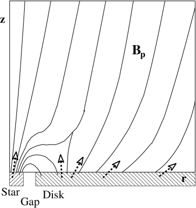
Figure 1: Scheme of model setup. Along the equatorial plane ($r$-axis) we distinguish jet inflow boundary conditions (shaded areas of ghost cells outside active grid) from the star ($r=0.0,...,r_{\star}=0.5$) and the disk region from $r_{i}=1.0,...,r=r_{\rm out}$). The mass flux from star or disk is prescribed by the profile for the inflow density and inflow velocity (dashed arrows). The latter is typically of about $0.1\%$ of the local Keplerian speed. The stellar boundary is in rigid rotation, the disk boundary in Keplerian rotation. The disk inner radius is at the co-rotation radius. In the gap area between disk and star ($r=0.5,...,r_{i}=1.0$) a minimum ”floor” mass flux is defined in order to keep the simulation going. Thin contours indicate initial poloidal field lines for one of the simulation runs.

2.2 Simulations of star-disk magnetospheres

The simulation of outflows from star-disk magnetospheres is a difficult numerical task due to strong gradients in magnetic field strength, density/pressure, and also the velocity field. Still, the first simulations of a stellar dipole surrounded by a disk have been presented in seminal papers as early as 1984 by Uchida & Shibata (1984, 1985). Probably due to the success of the disk wind models (Blandford & Payne, 1982; Pudritz & Norman, 1983) the formation of outflows from stellar magnetospheres became somewhat unattended before the topic was re-discovered in the early 90ies with several model suggestions (Camenzind, 1990; Shu et al., 1994). Numerical, stationary-state MHD solutions of the star-disk jet formation problem were presented subsequently (Fendt et al., 1995; Fendt & Camenzind, 1996; Sauty & Tsinganos, 1994).

Time-dependent simulations of dipolar magnetospheres started again later Hayashi et al. (1996); Hirose et al. (1997); Miller & Stone (1997). However, the time scale of these simulations including the disk evolution was short - a few inner disk rotations.

Goodson et al. (Goodson et al., 1997, 1999; Matt et al., 2002) in a series of papers presented simulations runs of dipolar star-disk magnetospheres for up to 150 (inner) disk rotations, in particular considering the reconnection/flaring behavior of the magnetic field close to the inner disk radius. As another result, a highly collimated, narrow jet emerged along the rotation axis for which the authors also presented forbidden emission line maps. Simulations by Matt et al. (2002) followed a similar setup, however, based on an increased grid scale of $(0.8\times 3.2\rm AU)$ and run for times scales of 150 days (stellar case). Magnetic flares emerging from the inner disk location lead to episodic mass ejections. These flares were both triggered and triggering a variation of the disk mass accretion rate and a corresponding change in the inner disk radius. Reconnection is strongly interrelated to magnetic diffusivity (resp. electric resistivity), however, such model assumptions were not particularly specified in these papers. Matt et al. (2002) investigated the setup of an ambient vertical field aligned with a central dipolar field. Their scenario is somewhat different to what we consider: the surrounding magnetic field is rather weak and vertical and, thus, not an active outflow-generating disk field as in our case. The authors identified three classes of field geometries - as in our setup depending on the direction of the ambient field. As a main result, in all three cases the collimation of the central outflow was observed, similar to earlier suggestions by Kwan & Tademaru (1988).

In comparison, Fendt & Elstner (1999, 2000) did not treat the disk structure in their simulations, allowing them to follow the evolution of the the stellar magnetosphere for more than 2000 rotation periods of the inner disk. These simulations showed for the first time that the axial jet feature observed in some of the simulations before (Miller & Stone, 1997; Goodson et al., 1997, 1999) is in fact an intermittent feature and disappears on the long term. The initial axial jet appears essentially during relaxation process of the hydrostatic initial condition towards a hydrodynamic steady state. Fendt & Elstner (2000) were first to introduce a physical stellar wind boundary condition in addition to the disk wind. The emerging two component outflow from star and disk remained un-collimated. This was understood as caused by the fact that no net electric current was driven along the outflow (since the initial dipolar field distribution). Since the stellar dipolar field becomes very weak along the disk, a classical magneto-centrifugal wind launching becomes inefficient. This is another reason for the lack of collimation observed in these simulations.

Simulations of the disk-star interaction Romanova et al. (2002); Küker et al. (2003); Romanova et al. (2004) focus on the dipolar accretion process and potential angular momentum exchange between star and disk. No evidence was found for persistent outflows and only episodic ejections from the inner disk area occurred. Time-dependent simulations of winds from an initially spherically symmetric stellar magnetic field were performed by Keppens & Goedbloed (1999), evolving exactly into the classical stationary Weber-Davis solution. Matt & Pudritz (2008) derive the angular momentum loss of pure stellar winds by numerical simulations. The setup is similar to the stationary-state models calculated by Fendt et al. (1995) and Fendt & Camenzind (1996). The outflow angular momentum loss derived from these simulations is comparable to what can be derived from the stationary models.

While the simulations from dipolar magnetospheres failed to show collimated outflows, MHD simulations of disk winds did actually proof the self-collimating characteristics of MHD winds. After seminal papers by Ustyugova et al. (1995) and Ouyed & Pudritz (1997) this approach was further developed taking into account the time-dependent change of disk field inclination (Krasnopolsky et al., 1999), turbulent magnetic diffusivity in the jet (Fendt & Cemeljic, 2002), a variation in the disk wind magnetic field and density profile (Pudritz et al., 2006; Fendt, 2006), or non-axisymmetric effects (Ouyed et al., 2003; Kigure & Shibata, 2005; Anderson et al., 2006), and also the disk dynamical evolution (Kudoh et al., 1998; Casse & Keppens, 2002; Kigure & Shibata, 2005; Zanni et al., 2007).

Recent simulations by Matsakos et al. (2008) investigated the ”topological stability” of two-component (star-disk) self-similar solutions derived from stationary MHD. In difference to our approach their simulations do not start from an initial hydro-static state, but from an initial dynamical steady state solution of the MHD equations, with analytical extrapolations in the case of radially self-similar solutions (which are singular on the axis). Meliani et al. (2007) presented two-component outflow simulations including the treatment of the disk evolution. However, although the wind dynamics indeed consists of two components, the magnetic field distribution basically resembled a monotonous field profile (i.e. no stellar dipole, no stellar outflow involved).

3 Simulation model setup

We perform axisymmetric MHD simulations of jet formation for a set of different magnetic field geometries and mass fluxes. The general model setup follows Ouyed & Pudritz (1997), Fendt & Cemeljic (2002) and Fendt (2006), however, with important modifications. The original ZEUS-3D ideal MHD code (Stone & Norman, 1992a, b; Hawley & Stone, 1995) extended for physical magnetic resistivity (see description and tests in Fendt & Cemeljic (2002)) is used. For the purpose of this paper the magnetic diffusivity was set to such a low level that it does not affect the overall collimation of the outflow. However, resistivity/diffusivity is essential for our simulations, as it allows for magnetospheric reconnection phenomena.

The set of MHD equations considered is the following,

$${\frac{\partial\rho}{\partial t}}+\nabla\cdot(\rho\vec{v})=0,\quad\nabla\cdot\vec{B}=0,\quad\frac{4\pi}{c}\vec{j}=\nabla\times\vec{B},$$ (3)

$$\rho\left[{\frac{\partial\vec{u}}{\partial t}}+\left(\vec{v}\cdot\nabla\right)\vec{v}\right]+\nabla(p+p_{A})+\rho\nabla\Phi-\frac{\vec{j}\times\vec{B}}{c}=0,$$ (4)

$${\frac{\partial\vec{B}}{\partial t}}-\nabla\times\left(\vec{v}\times\vec{B}-{\frac{4\pi}{c}}\eta\vec{j}\right)=0,$$ (5)

$$\rho\left[{\frac{\partial e}{\partial t}}+\left(\vec{v}\cdot\nabla\right)e\right]+p(\nabla\cdot\vec{v})-{\frac{4\pi}{c^{2}}}\eta\vec{j}^{2}=0,$$ (6)

with the usual notation for the variables (see Fendt & Elstner (2000); Fendt (2006)). The magnetic diffusivity is space and time dependent and is denoted by $\eta(r,z)$.

We apply a polytropic equation of state for the gas with the polytropic index $\gamma=5/3$. As (Ouyed & Pudritz, 1997) we have added turbulent Alfvénic pressure in order to allow to keep the corona ”cool”. In fact, we do not solve the energy equation 6 and apply the internal energy of the gas reduced to $e=p/(\gamma-1)$. Two major reasons to do this are both computational speed and numerical stability. Some of our long-term simulations did last already more than two months of CPU time and it would be impossible to reach the desired evolutionary steps if the energy equation would have been solved. Following Ouyed & Pudritz (1997) this approach also allows to combine gas pressure forces and gravity under the same derivative in the code. Thus, instead of subtracting gradients, we apply the gradient of the difference, which results in perfect stability of the initial state. Note, however, that recent work by Clarke and collaborators seems to indicate that relaxation of the polytropy assumption may affect the dynamical evolution in certain domains of the jet, in particular regions with shocks or contact discontinuities (Ramsey & Clarke, 2004).

The magnetic diffusivity can be considered as turbulent and, thus, be related to the Alfvénic turbulent pressure $p_{\rm A}$ if we assume that it is primarily due to the turbulent Alfvénic waves which are responsible for the turbulent Alfvénic pressure applied in the simulations. In our previous work (Fendt & Cemeljic, 2002) we have derived a toy parameterization relating both effects by parameterizing the turbulent magnetic diffusivity similar to the Shakura-Sunyaev parameterization of turbulent viscosity, ${\eta}_{\rm t}=\alpha_{\rm m}vl$, where $\alpha_{\rm m}\leq\!1$ and $l$ and $v$ are the characteristic dynamical length scale and velocity of the system, respectively. With that we obtain ${\eta}_{\rm t}=\alpha_{\rm m}v_{\rm t}l$ and with ${\beta}_{\rm t}=(c_{\rm s}/v_{\rm t})^{2}$ and $c_{\rm s}^{2}=\gamma\,p/\rho$, it follows that $v_{\rm t}^{2}=\frac{\gamma}{{\beta}_{\rm t}}\frac{p}{\rho}$, or, normalized, ${v^{\prime}}_{\rm t}^{2}=\frac{\gamma}{{\delta}_{\rm i}{\beta}_{\rm t}}\rho^{\prime\gamma-1}$. For the chosen polytropic index this implies a magnetic diffusivity $\eta\sim\rho^{1/3}$ if $l$ is constant (see also the discussion in Fendt (2006)). We again stress the point that in the present paper the magnetic diffusivity is on a such a low level (much below the critical level found in Fendt & Cemeljic (2002)) that it does not affect the dynamics, but allows for reconnection.

For the numerical grid, we use the “scaled grid” option by ZEUS with the element size decreasing inwards by a factor of 0.99. The size of the cylindrical grid is $(256\times 256)$ elements resulting in a physical grid size for all simulations is $(r\times z)=(80\times 80)r_{\rm i}$ corresponding to $(4\times 4)$ AU for $r_{\rm i}\simeq 10\,{\rm R}_{\sun}$. Thus, the disk gap ($r<1$) is resolved with 11 grid elements. Time is measured in rotation periods (Keplerian orbits) at the inner disk radius.

In summary, compared to our previous studies (Fendt & Elstner, 2000; Fendt & Cemeljic, 2002; Fendt, 2006), the main new feature included in the present approach is that the initial magnetic field distribution consists of two components - a stellar dipolar field and a disk field. In difference to recent studies by (Meliani et al., 2007) we included both outflow components and magnetic field components in the simulation box, in particular treating the star-gap-disk boundary.

3.1 Boundary conditions

Along the $r$-boundary we distinguish between the star extending from $r=0.0$ to $r=r_{\star}=0.5$, the gap region extending from $r=0.5$ to $r=r_{i}=1.0$, and the disk region from $r=1.0$ to $r=r_{\rm out}$, see Fig.1. A Keplerian disk is taken as a (fixed in time and space) boundary condition for the mass inflow from the disk surface into the corona and the magnetic flux. The stellar surface is approximated by a rigidly rotating ”disk” in cylindrical coordinates. The stellar rotation is chosen such that the inner disk radius is located at the co-rotation radius.

The initial magnetic field is purely poloidal. Magnetic field lines are anchored in the disk and the rotating star and are in co-rotation with their respective foot point. The poloidal magnetic field profile along the $r$-boundary remains fixed in time and is, hence, determined by the choice of the initial magnetic field distribution.

The disk region governs the mass inflow from the disk surface into corona (denoted as ”disk wind”). In addition to that we prescribe a stellar wind with different mass load. The hydrodynamic boundary conditions are “inflow” along the $r$-axis for the disk and stellar region and either ”inflow” (very light mass flow) or ”reflecting” for the gap region, “reflecting” along the symmetry axis and “outflow” along the outer boundaries. Matter is “injected” from the disk and the star into the corona parallel to the poloidal magnetic field lines with very low velocity $\vec{v}_{\rm inj}(r,0)=\nu_{\rm i}v_{\rm K}(r)\vec{B}_{\rm P}/B_{\rm P}$ and with a density $\rho_{\rm inj}(r,0)=\eta_{\rm i}\,\rho(r,0)$. The proportionality constants are typically $\nu_{\rm i}\simeq 10^{-3}$ and $\eta_{\rm i}\simeq 100$ for both, stellar and disk wind (but usually different for both components). Along the gap we impose a floor value for the density $\eta_{\rm i}\simeq 10^{-3}$ and a similarly low velocity. For the injection velocity, the assumption is that the initial disk wind speed is in the range of the sound speed in the disk, $v_{\rm inj}(r)\simeq c_{\rm s}(r)\simeq v_{\rm kep}\sim r^{-1/2}$.

These mass loss rates from star and disk, respectively, are our other main parameters besides the respective magnetic flux (see Tab. 1).

Figure 2: Example initial magnetic field distributions. Shown are poloidal magnetic field lines. Full and dashed lines indicate the direction of magnetic flux. The plots show different options for the strength and orientation of the superposed stellar and disk magnetic field components $\Psi_{0,\rm d}=0.01,-0.01,-0.1,$ resp. $\Psi_{0,\star}=5.0,5.0,3.0$ (from top to bottom; runs A2, A3, A4a).

3.2 Initial conditions

As initial state we prescribe a force-free magnetic field along with a gas distribution in hydrostatic equilibrium. Both is essential in order to avoid artificial relaxation processes caused by a non-equilibrium initial condition. The initial density distribution is $\rho(r,z,t=0)=(r^{2}+z^{2})^{-3/4}$. As initial magnetic field distribution we superpose a dipolar stellar field and a disk potential field. For the disk field component we apply the model of Ouyed & Pudritz (1997) and Fendt & Cemeljic (2002). We prescribe the magnetic field distribution as derivative of the magnetic flux distribution $\Psi(r,z)\equiv\int\vec{B}_{\rm p}d\vec{A}$ (i.e. the $\phi$-component of the vector potential). For the superposed magnetic flux from star and disk we have

$$\Psi(r,z)=\Psi_{0,\rm d}\,\frac{1}{r}\left(\sqrt{r^{2}+(z_{\rm d}+z)^{2}}-(z_{\rm d}+z)\right)$$

$$+\Psi_{0,\star}\,\frac{r^{2}}{\left(r^{2}+(z_{\rm d}+z)^{2}\right)^{3/2}},$$ (7)

with the stellar and disk magnetic flux $\Psi_{0,\star}$ and $\Psi_{0,\rm d}$. The poloidal magnetic field follows from the derivatives $B_{\rm r}=-(1/r)(\partial\Psi/(\partial z)$ and $B_{\rm z}=(1/r)(\partial\Psi/(\partial r)$, properly calulated in the staggered mesh in order to obtain a numerically divergence-free and force-free initial field structure. The dimensionless disk thickness $z_{\rm d}$ with $(z_{\rm d}+z)>0$ for $z<0$ is introduced in order to avoid kinks in the field distribution. Several combinations of both field components were investigated, parameterized by combinations of $\Psi_{0,\rm d}$ and $\Psi_{0,\star}$. Figure 2 shows three examples for the initial field configuration for different strength and alignment of the field components. Similar field geometries have been discussed already by Uchida & Low (1981). Matt et al. (2002) did consider similar configurations, however, superimposing a stellar dipole with a weak vertical disk field.

In order to allow for a clear comparison between all our runs, the respective magnetic field component profiles and wind density component profiles are identical.

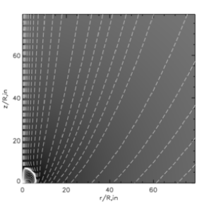
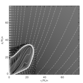
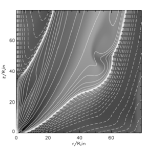
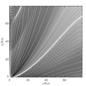
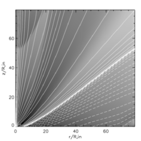
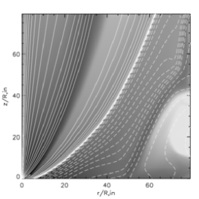
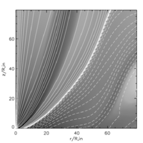
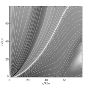
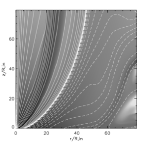
Figure 3: Time evolution of simulation run A4a. Poloidal magnetic field distribution at time steps $t=0,50,200,500,1000,2000,2500,3000,3600$ (from top left to bottom right). Density gray scale as indicated. Poloidal field lines as contour levels of the magnetic flux, $-\Psi(r,z)=$ 3.0 ,2.0 ,1.6 ,1.3, 1.0, 0.8, 0.6, 0.4, 0.2, 0.12, 0.064, 0.032, 0.016, 0.008, 0.004, 0.002, 0.001, 0.0005, 0.0002, 0.0001, (dashed), $\Psi(r,z)=$ 0.0002, 0.0005, 0.001, 0.002, 0.004, 0.008, 0.016, 0.032, 0.064, 0.12, 0.2, 0.3, 0.4, 0.6, 0.8, 1.0, 1.3, 1.6, 2.0 (solid).

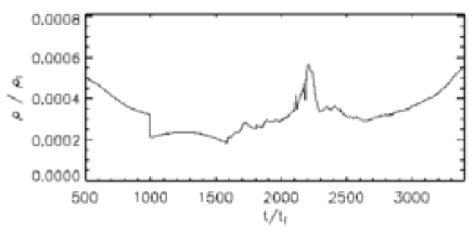
Figure 4: Time evolution of the density at $z=44,r=44$ for simulation run A4a.

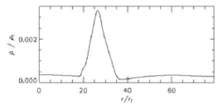
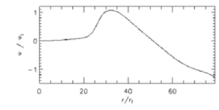
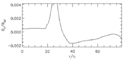
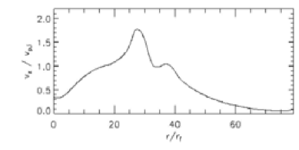
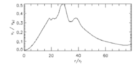
Figure 5: Radial profiles of density, magnetic flux, axial magnetic field, axial velocity, and radial velocity (from top to bottom) at $z=55$ for simulation run A4a at $t=3000$. Note the neutral field line (magnetic field reversal) at $r\simeq 33$ and the magnetic flux reversal at $r\simeq 53$.

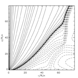
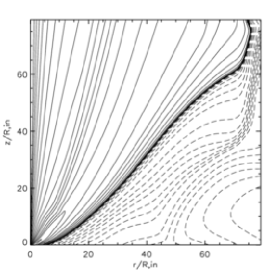
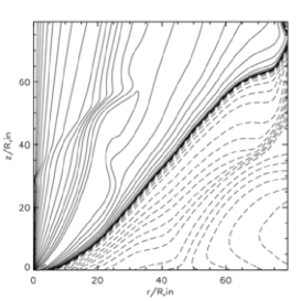
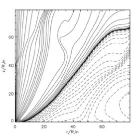
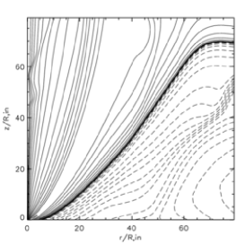
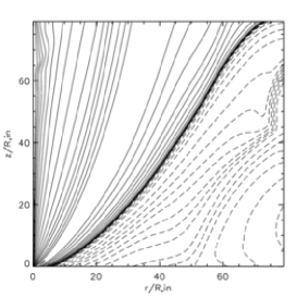
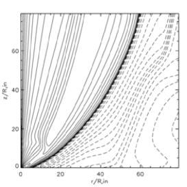
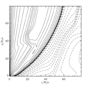
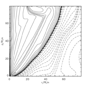
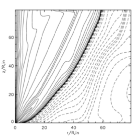
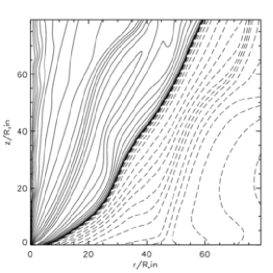
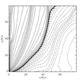
Figure 6: Poloidal magnetic field evolution during two flares around $t=176$ and $t=210$. Solid and dashed lines indicate the direction of total magnetic flux of the superposed dipolar and disk magnetic field components. Shown are time steps: 1700, 1760, 1790, 1810, 1840, 1890, 2080, 2100, 2130, 2140, 2180, 2250 (from top left to bottom right) of simulation A4a. Contour levels as in Fig. 3.

4 Results and discussion

We now discuss a number of MHD jet formation simulations covering a wide parameter range (see Tab. 1) concerning both the magnitude of the disk and stellar wind mass load and magnetic flux, respectively. The results presented here are preliminary in the sense that not all simulation runs could be performed over time scales sufficiently long enough for the MHD flow as a whole to reach the grid boundaries or to establish a stationary state. This is due to the comparatively large physical grid size in combination with steep gradients in the disk wind parameters which in general allow only for a weak outflow from large disk radii. In particular the steep decline of the stellar field in combination with a reasonable disk mass loss rate is numerically problematic (see below). Therefore, for a true comparison between different runs it is essential to also take into account the dynamical state of the outflow.

In order to check for resolution issues, we have also run a set of simulations with twice the resolution, without seeing significant differences (runs A4b, A5, A6). Thus, since we are interested in many parameter runs evolving for a long time, we mainly concentrate on the lower resolution simulations. We describe first the general evolution of jet formation in our simulations (see also (Ouyed & Pudritz, 1997; Fendt & Cemeljic, 2002; Fendt, 2006)) and later discuss specific features.

4.1 Overall evolution of an outflow

Figure 3 shows how the field structure evolves in time for the simulation run A4a. In this case the stellar dipolar field and the disk field are aligned. Thus, the X-point is initially along the rotational axis. We have stopped this simulation after 3600 Keplerian rotations at the inner disk radius. This corresponds to 6 rotations at the outer disk radius and makes it clear that the outer parts of the disk wind have not yet completely evolved into a quasi-stationary state. This is a generic problem of all disk-jet simulations published so far as soon as large disk radii are considered.

The evolution during the very first time steps from the initial shows that above the emerging outflow the initial steady state corona is still present. The X-point which was initially located at $z<10$ along the rotational axis, moves upwards to $z\simeq 20$ (for $t=50$) and $z\simeq 40$ (for $t=200$) and is later swept out of the computational domain for $t>600$ (see top of Fig. 3 and discussion end of Sect.4.2).

Since the initial condition is still kept in steady state, artificial dynamical re-configuration is prevented. This demonstrates that the numerical resolution is sufficient for our problem also in the out parts of the grid.

The next dominant feature is observed still at early stages of about ten rotations. The initial dipolar field breaks up due to the magnetic pressure of the toroidal magnetic field induced by differential rotation between star and disk. The magnetic pressure gradient drives this outflow. Furthermore, an intermediate axial jet is launched due to the re-arrangement of the initially hydrostatic corona to a new dynamical equilibrium state. In fact, as the magnetic field along the axis is squeezed by lateral dynamical pressure, the material is accelerated along the rotational axis. After the dipole is broken up, there is few direct magnetic connection between star and disk anymore and the differential rotation induced toroidal field decreases.

The outflows from star and disk continue to grow gaining higher kinetic energy and momentum. MHD self-induction of toroidal magnetic field leads to collimation and magnetic acceleration. Compared to pure disk winds (Ouyed & Pudritz, 1997; Fendt & Cemeljic, 2002; Fendt, 2006) the outflow is clearly less collimated as being de-collimated by the central stellar wind.

At intermediate time scales quasi-stationary states may emerge. This is demonstrated for example in simulation A4a in Fig. 4 by showing the time evolution of the density at point $(z=44,r=44)$. Two plateaus are clearly seen at different density levels indicating two quasi-stationary states of the flow evolution. One is from $t\simeq 1000$ till $t\simeq 1500$, the other from $t\simeq 2300-3000$ when the outflow is slowly re-adjusting from the flaring events (see below). Note, however, that at this time the outer disk has rotated only about a fifth of an orbit. Thus, the field and flow above the outer disk will further evolve in time and again disturb the enclosed structure in quasi-steady state. We observe that over even longer time scale such quasi-stationary states may be reached (and be disturbed) again and probably again and again. We believe that this feature is due to the still ongoing evolution of the outer disk wind. The final states of some representative simulation runs are shown in Fig. 13 and 14. We will discuss them in Sect.4.4.3 below.

As seen already from the initial field configuration, the simulations of the anti-aligned field configuration (as e.g. A4a) reveal a change of sign in the magnetic flux distribution from star and disk (negative magnetic flux is indicated by dashed contours in Fig. 5). The location of flux reversal is accompanied with a concentration of contour lines in our figures which may be confused with the existence of a shock. This is however an artifact of the choice of contour levels for the magnetic flux. In fact, it makes sense to follow the same field lines emerging from the stellar surface also back into the disk surface. Since the strong gradient of the stellar dipolar field, magnetic flux levels aroung $\Psi=0$ are concentrated. Figure 5 shows that the radial profiles of density, velocity and poloidal field accross the flux reversal. Note that the location of magnetic field reversal (the neutral field line) is at a smaller radius $r=33$ compared to the magnetic flux reversal at about $r=53$. Within the magnetic field reversal magnetic flux is accumulated. Beyond the field reversal the magnetic flux decreases and then becomes negative.

4.2 Reconnection and large scale flares

Our version of ZEUS code has physical magnetic diffusivity implemented (see Fendt & Cemeljic (2002) for explanation and tests). This allows to consider reconnection processes.

We observe reconnection flares along some of the outflows (see Fig. 6). These flares are similar to coronal mass ejection. They rapidly evolve and propagate along the neutral field line. Once formed, reconnection islands (or rather ”tori” in our axisymmetric setup) propagate across the jet magnetosphere within a few rotation times and leave the computational domain. The flares typically expand and reconnect within 70 time units equivalent to 70 orbital periods of the inner disk (and 70 stellar rotations). We may also naively measure the flare propagation speed by the proper motion of the field lines observed in the simulation. This gives an average ”flare propagation speed” of about unity, as they travel 80 spatial units in 70 time units - the Keplerian speed at their foot-point. The flares propagate along the neutral field line, and leave the physical grid at a radius corresponding to about 7-10 AU from the axis.

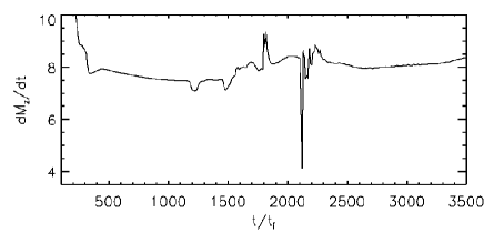
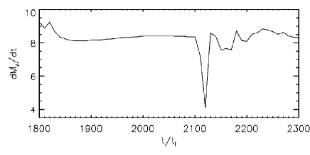
Figure 7: Integrated mass flux in axial direction across the upper $z$-boundary versus time. Note the change of mass flux of about $10-50\%$ during the flare events. The high mass flux for $t<500$ indicates sweeping off of the initial hydrostatic corona.

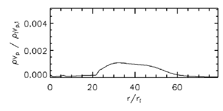
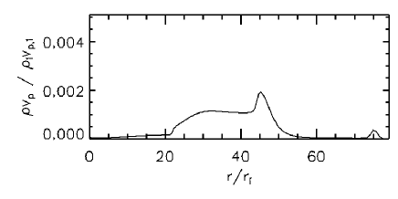
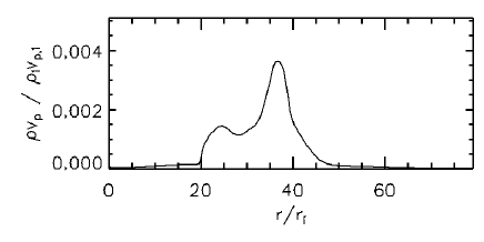
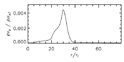
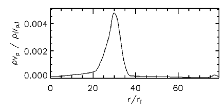
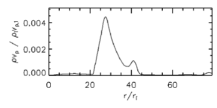
Figure 8: Profile of the outflow momentum along the z-boundary at time $t=1400,1600,1800,1900,2100,2200,2500,3000$. Note the re-distribution of the main mass flow channel from radius $r=60$ to $r=40$.

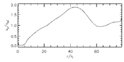
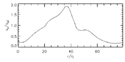
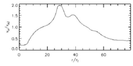
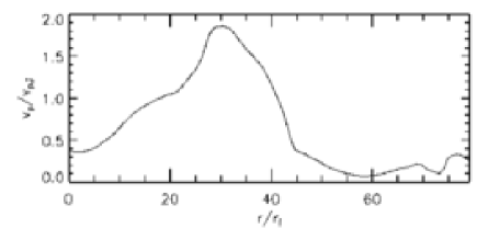
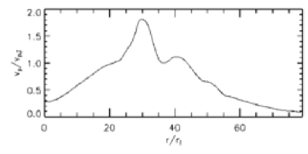
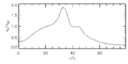
Figure 9: Profile of the axial outflow velocity along the z-boundary at time $t=1400,1800,1850,2200,2300,3000$.

In the following we mainly concentrate on simulation A4a. Figure 11 is a magnification of the inner area of Fig.6 and demonstrates that the flares are actually from a Y-point above the disk, located at ($z\simeq 2,r\simeq 4$) Note that the stellar magnetosphere remains closed also for foot-points along the disk with $r<3$ (at $t\simeq 1700$), respectively $r<2$ ($t\simeq 1700$), beyond the co-rotation radius. In this case the flare eruptions are launched close to the inner disk area, but not at the inner disk radius.

Goodson et al. (1999) also observed flares or reconnection events in their simulations of a dipolar magnetosphere connected top a surrounding accretion disk. Since the evolution of the disk structure was treated in their simulation, they were able to observe time-dependent accretion along the equatorial plane. The frequent ejection events of AU-sized knots along the rotational axis were correlated with a time-variation of the accretion rate. This is different in our case, where the reconnection/flares seem to be triggered by the evolution of the outer disk wind. As mentioned, during the run-time of our simulations (up to 3600 inner disk rotations) the corona (or disk wind respectively) above the outer disk has not yet reached a steady dynamical state. Thus, in our case, as the outer disk outflow evolves, the cross-jet pressure equilibrium is changed and forces the inner magnetic field configuration to adjust accordingly. Since Goodson et al did not specify the distribution and magnitude of the magnetic diffusivity in their simulations, it is difficult to compare the results in detail. Another difference is the duration of the simulation. While our physical grid size is only marginally larger, the time scale of our simulations is substantially longer (3600 inner disk rotations corresponding to about 36,000 days compared to 130 days). This is particularly important when considering the dynamical evolution above the outer part of the disk and the long-term behavior.

The flare events observed in our simulations are accompanied by a temporal change in outflow mass flux, velocity, or momentum, respectively. Figure 7 shows the mass loss rate in axial direction integrated across the upper r-boundary versus time. During the first flare we see a 10%-variation in the mass flux followed by a sudden decrease of mass flux by a factor of two during flare two. Figures 8 and 9 show the profiles of jet momentum and poloidal velocity across the upper r-boundary. We see that during flaring these profile indicate a re-arrangement of momentum and velocity profile across the jet. Before the flare, the radial jet momentum profile is broad (see Fig. 8 upper left for $t=1400$). In fact, the profile (Fig. 8, $t=1400$) remains very similar for several 100 rotations before until the flare event starts. After the flare has passed the grid, the jet momentum profile is concentrated within a cylindrical sheet of radius $r\simeq 35$ and thickness $\Delta r\simeq 5$ (Fig. 8 lower right at $t=2300$). Similar to the situation before the flare, the jet momentum profile for time steps after the flare ($t>2300$) look almost identical (see bottom sub-figures for $t=2600$ and $t=3000$).

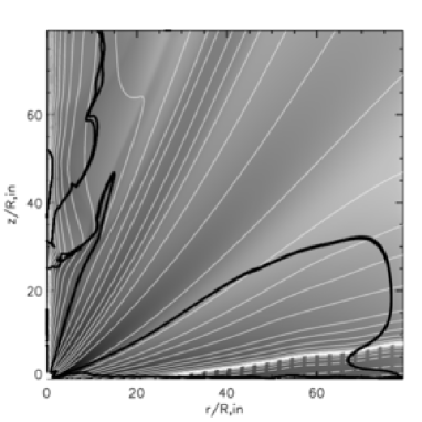
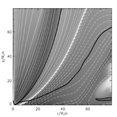
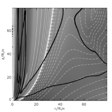
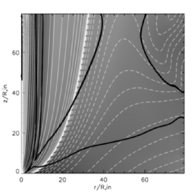
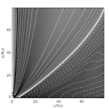
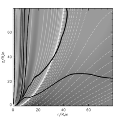
Figure 14: Poloidal magnetic field distribution at the time when the simulation was stopped. Simulation A3 (t=500); A4a (t=3200); A10 (t=550); A13 (t=620); A12 (t=380); A14 (t=660) (from top left to bottom right). Contour levels and grey scale as in Fig. 3.

This behavior is somewhat mirrored in the poloidal velocity profile. What is interesting for shock formation in the asymptotic jet, is a temporal change in jet velocity at certain jet radii (see below). The maximum velocities in the outflow reach about two times the Keplerian speed at the inner disk radius and vary by a factor of two. Along the neutral field line the outflow velocity is fast-magnetosonic (see Figs. 11 and 14 where the fast surface is indicated).

As an estimate for the reconnection time scale we may apply the Sweet-Parker approach with $\tau_{\rm SP}\simeq\sqrt{\tau_{\rm A}\tau_{\rm diff}}$ with the dynamical (Alfvén) time scale $\tau_{\rm A}=l/v_{\rm A}$ and the diffusive time scale $\tau_{\rm diff}=l^{2}/\eta$. With our model of turbulent magnetic diffusivity $\eta=\eta_{0}\rho^{1/3}$ we find $\tau_{\rm SP}\simeq l^{3/2}(4\pi)^{1/4}\eta_{0}^{-1/2}\rho^{1/12}$. For $\eta_{0}=0.01$, and $\rho\simeq 0.02$ at the reconnection area with $l\simeq 2$ (for simulation A16) that $\tau_{\rm SP}\simeq 30$. This is similar to the duration of the reconnection flare we observe between $t=600$ and $t=650$.

Note an interesting feature in both of the general model setups (aligned and anti-aligned field geometry) concerning the reconnection geometry. Figures 11 and 12 show the inner structure of the star-disk magnetosphere. These simulations (A04a, A16) were launched from differently aligned field geometries (aligned/anti-aligned disk-stellar field). In the anti-aligned case the initial X-point is along the axis. However, as the magnetic field evolves, the dipole expands and sweeps off the initial field along the axis. A new X-point evolves by disruption of some of the closed dipolar field loops. The new X-point is located above the disk close to the inner disk radius (see above). This situation is not very different from the the aligned case for which the initial X-point, located along the equatorial plane, moves up to a certain (small) height above the disk. In summary, our simulations show that no magnetic X-point remains along the equatorial plane as e.g. assumed in the Shu et al. X-wind model. Instead we find from both initial configurations an X-point above the disk (sometimes also called Y-point, (Ferreira et al., 2006)), located at time-averaged distances ($z\simeq 4,r\simeq 2$) or ($z\simeq 8,r\simeq 2$), respectively.

4.3 Flaring events as jet knot generator?

The generation of knots in protostellar jets is a long-standing puzzle. In particular, it is unclear whether the shocks/knots are triggered by the internal engine or due to interaction with the ambient medium. A strong argument for the first possibility is the existence of some perfectly symmetric jets as HH 212 (Zinnecker et al., 1998), however, the majority of jet sources looks asymmetric. Internal shocks along the jet flow may be caused e.g. by a time-dependent velocity variation of the material injected into the jet (e.g. Raga et al. (2007)). Even if we have observational support for the idea of the jet knots being triggered by the central engine, we do not know how the central engine does that. The time scale derived from typical knot separations $d_{\rm knot}$ and velocities $v_{\rm knot}$ correspond to

$$t_{\rm knot}=10\,{\rm yrs}\left(\frac{v_{\rm knot}}{300\,{\rm km/s}}\right)\left(\frac{d_{\rm knot}}{100\,{\rm AU}}\right)$$ (8)

which is clearly different from the Keplerian time scale close to the inner disk edge from where the jets are launched.

Considering the ejection of large-scale flares and the follow-up re-arrangement of outflow density and velocity distribution in our simulations, one is tempted to hypothesize that the origin of knots is triggered by such flaring events.

In our simulations (A4a, A16) the time scale of flare generation is about 500-1000 rotational periods of the inner disk, corresponding to about 30-60 years (assuming an inner disk rotation period of, say two times the co-rotation period of a typical T Tauri star of about 10 days). The variation in the hydrodynamic parameters lasts for about 30-40 inner disk rotation times (respectively about $<400$ days for a 10 day stellar rotation period). The further evolution and generation of further flaring events is of course not known as it is beyond our computation time. The essential point, however, is that we detect a long time scale, substantially longer than the typical dynamical time scales at the jet formation area. That time scale is surprisingly similar to the time scale defined by the observed knot separation and velocity. Of course, it is to early to draw firm conclusions from such a tentative agreement. The reconnection time-scale is governed by the magnetic diffusivity for which we have applied our self-consistent model of turbulent magnetic diffusivity (Fendt & Cemeljic, 2002).

It is left to further simulations of the asymptotic collimated jet beam to check whether the detected variation in outflow speed and mass flux (Figs. 7,8,9) is sufficient in order to generate strong internal shocks comparable to the observed knots.

4.4 Collimation degree, mass loss rate and field alignment

In this section we compare the overall collimation behavior of the different simulation runs. In previous studies (Fendt & Cemeljic, 2002; Fendt, 2006) we quantified the degree of outflow collimation $\zeta$ by comparing the mass flow rates in axial and lateral direction,

$$\zeta\equiv\frac{\dot{M}_{\rm z}}{\dot{M}_{\rm r}}={{2\pi\int_{0}^{r_{\rm max}}r\rho v_{z}dr}\over{2\pi r_{\rm max}\int_{0}^{z_{\rm max}}\rho v_{r}dz}.}$$ (9)

In Tab. 1 we provide mass flow rate within four differently sized volumes, $\dot{M}_{{\rm z},i},\dot{M}_{{\rm r},i}$, considering different sub-grids of the whole computational domain, i.e.cylinders of radius and height $(r_{\rm max}\times z_{\rm max})=(12\!\times\!12),(24\!\times\!24),(43\!\times\!43)$, and $(76\!\times\!76)$. We calculate the mass fluxes ratio normalized to the size of the area threaded by the mass flows in r- and z-direction, $\hat{\zeta}_{1},\hat{\zeta}_{2},\hat{\zeta}_{3},\hat{\zeta}_{4}$. The ratio of grid extension $(r_{\rm max}/z_{\rm max})$ as displayed in our figures converts into a ratio of cylinder surface areas of $A_{\rm z}/A_{\rm r}\sim 0.5(r_{\rm max}/z_{\rm max})$. As a general measure of collimation degree, we give an average value $<\zeta>$ which may consider also the dynamical state of the simulation run.

Compared to our previous work on pure disk wind collimation, where the relative mass flux of the collimating disk wind is a sufficient quantitative measure of collimation the situation in the present setup is not exactly the same. Naturally, the stellar wind mass flux emerges close to the outflow axis and will tend to stay close to it. Thus, a high stellar mass flux will naturally cause a more collimated mass flow.

In order to compare the collimation degree within the large volume, it is essential to check the evolutionary state of the flow. In all of our simulation runs the initial corona has completely swept out of the grid. In this case, all of the mass flux we measure has been launched by the disk wind. Exceptions are simulations A10, A13, and A12, where a relict of the initial bow shock are still visible in the outer layers. The mass loss rates in these examples have to taken with care, at least the values from the larger volumes. Run A16 is evolving very slowly in the outer part and it was not possible within reasonable CPU time to evolve the disk wind to larger distances from the disk surface.

4.4.1 Collimation along the outflow

The degree of collimation derived from the simulations is in general different for the the different volumes, $\hat{\zeta}_{1},\hat{\zeta}_{2},\hat{\zeta}_{3},\hat{\zeta}_{3}$.

In most cases, the degree of mass flux collimation increases along the flow which is exactly the signature of MHD self-collimation. The outflow starts as un-collimated disk/stellar wind, and reaches the outer grid boundaries as collimated beam.

A good example is simulation A7, where the collimation of mass flow changes from ration $\sim 0.3$ for the inner region to $\sim 7$ in the outer parts. The same arguments hold for simulations A8, A15, A14. A similar behavior is seen e.g. in simulations A10, A13, A14, however, the collimation in mass flux around the largest volume is low. In these cases the outermost flow structure has not yet evolved into a steady state and either parts of the initial bow shock or the initial corona are still in the computational domain.

A counter example is simulation A12, which stays un-collimated in mass flux, although the magnetic field distribution looks collimated. Simulation A12 is exceptional for its high mass flux launched from the disk surface. Thus, the disk wind starts super-Alfvénic and super-seed the magnetosonic speed quickly. The standard Blandford-Payne magneto-centrifugal acceleration is not very efficient in this case, which also results in only little induction of toroidal magnetic field and, thus, Lorentz force, see Fig,10. The radial component of the perpendicular Lorentz force component is negative, i.e. directed inwards, however, too weak to balance the strong inner centrifugal force, resulting in a weak collimation of the outer part.

Table 1 shows also the time evolution of the collimation degree. Example A15 demonstrates how the collimation degree progresses in time. From earlier times (t=550) to later times ($t=2100$) collimation increases as the outflow evolves into a new dynamical state over the whole numerical grid. The same hold for example A14 and others. Examples A7, A8, A9 are calculated for a high stellar wind mass load, thus the time-evolution of the outer disk wind does not play a big role concerning collimation. This outflows reach a high degree of collimation early in time.

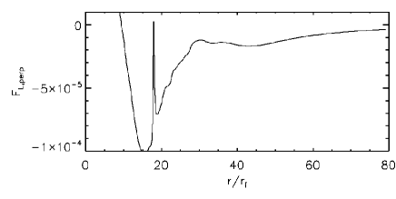
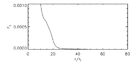
Figure 10: Perpendicular Lorentz force (top) and centrifugal force (bottom) across simulation A12 at height $z=50$ at time $t=380$.

4.4.2 Collimation and mass loss rates

The mass loss rates from star and disk are prescribed as boundary condition. A higher mass load in the stellar wind component would naturally result in a higher degree of collimation in the mass flux as this mass is just launched closer to the outflow axis.

Simulations A2 and A3 are good examples. The stellar wind mass loss is 2-3 times the disk wind mass flux. The resulting mass flux ratio is similar, thus this outflow is rather well collimated hydrodynamically. However, in spite the quite good collimation in mass flux, the magnetic field structure is not collimated with almost (spherical) radially expanding poloidal field lines (see Fig. 13). The field structure (and thus the poloidal velocity field) has a conical shape and is thus un-collimated. Similar as for simulation A12 (see above) the disk wind is too weak in order to collimate the stellar wind to a high degree.

Simulations A12 and A13 have the same star-disk magnetic field profile, however with a different mass load by a factor of ten. Run A12 reaches the same dynamical evolutionary state as A13, but earlier at $t=300$ instead of $t=620$. The less magnetized outflow A13 is stronger collimated. Run A14 has the same mass load as A13, but the double magnetic flux resulting in similar collimation degree.

Simulations A10 and A13 differ only by the stellar wind mass load (factor two), however this mass load is low and does not result in a variation of the overall degree of collimation. Note that for both simulations, the outer area of the outflow has not yet evolved in a steady state and a relict from the initial bow shock are still visible.

4.4.3 Collimation and magnetic field alignment

From the technical point, the simulation of the case where magnetic dipole and disk magnetic field are anti-aligned (A3, A4, A10, A13, A12, A14) are computationally less expensive and were therefore able to evolve to considerably longer time.

For the aligned cases (A9, A8, A7, A16, A15, A2) only the less magnetized evolve into a quasi stationary state in the outer (disk) outflow in reasonable time. We mention in particular run A15 with a reasonably strong disk magnetic flux which enables a collimating disk wind (compare to A16 and A7).

Simulations A9, A8 and A7 demonstrate that a low mass flux disk wind mass flux cannot evolve into a collimated disk wind even if the magnetic flux is relatively high if it is dominated by a strong central stellar jet.

The most promising model setup in order to explain strong stellar jets from a star-disk magnetosphere are those with relatively strong disk wind and disk magnetic flux. The stellar wind dominated simulations may give a high degree of collimation, however they collimate to too small radii. Stellar magnetic flux dominated simulations tend to stay un-collimated.

Figure 11: Poloidal magnetic field distribution (thin lines) during flare evolution (run A04). Contour levels as in Fig. 3. Simulation time steps t=2000, 2060, 2070, 2130, 2140, 3000. (from top left to bottom right). Alfvén and fast surface are shown by thick lines. Note the super-Alfvenic /super-fast stellar wind.

Figure 12: Poloidal magnetic field distribution (thin lines) during flare evolution (run A16). Contour levels as in Fig. 3. Simulation time steps t= 600, 620, 630, 640, 670, 760. (from top left to bottom right). Alfvén and fast surface are shown by thick lines. Note the super-Alfvenic /super-fast stellar wind.

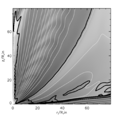
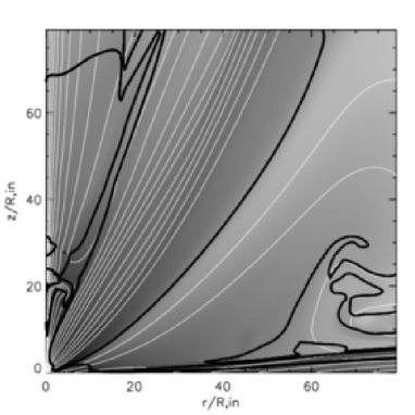
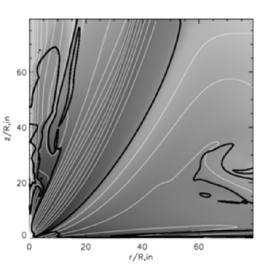
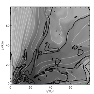
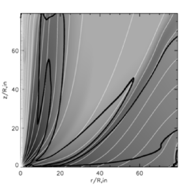
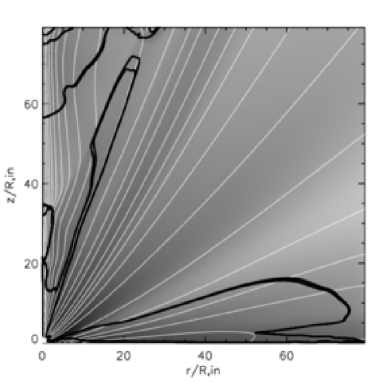
Figure 13: Poloidal magnetic field lines at the time when the simulation was stopped. Simulation A9 (t=740); A8 (t=1000); A7 (t=1400); A16 (t=1350) A15 (t=2100); A2 (t=700) (from top left to bottom right). Thick and medium thick lines indicate the location of the Alfvén and the magnetosonic surface. Contour levels and grey scale as in Fig. 3.

Table 1: Summary of simulation runs ID. Shown are disk and stellar mass loss rates, ${\dot{M}_{\rm d}},{\dot{M}_{\star}}$, corresponding magnetic fluxes, $\Psi_{0,\rm d},\Psi_{0,\star}$, and the physical time step $\tau$, when the collimation degree has been calculated. Mass loss rates $\dot{M}_{{\rm z}i},\dot{M}_{{\rm r}i}$ in $z$- and $r$-direction are integrated along three sub-grids $(r_{i,{\rm max}}\times z_{i,{\rm max}})=(11.6\times 11.6),(23.6\times 23.6),(43.4\times 43.4),(76.2\times 76.2),$ (for the $(80.0\times 80.0)$ grid). The average degree of collimation $<\!\!\zeta\!\!>$ is defined by the relative mass fluxes in $z$ and $r$-direction, normalized by the area threaded. Simulations labeled with a ’*’ were run on a smaller, higher resolution $(40.0\times 40.0)$ grid.

ID	${\dot{M}_{\rm D}}\over{\dot{M}_{\star}}$	$\Psi_{0,disk}$	$\Psi_{0,\star}$	$\tau$	$\dot{M}_{z1},\dot{M}_{r1}$	$\dot{M}_{z2},\dot{M}_{r2}$	$\dot{M}_{z3},\dot{M}_{r3}$	$\dot{M}_{z4},\dot{M}_{r4}$	$\hat{\zeta}_{1},\hat{\zeta}_{2},\hat{\zeta}_{3},\hat{\zeta}_{4}$	$<\!\!\zeta\!\!>$
A9	${1.55}\over{5.62}$	0.1	10.0	740	2.37, 5.82	4.72, 3.87	6.42, 1.64	7.44, 1.09	0.41, 1.2, 3.9, 6.8
				700	2.90, 5.99	4.73, 4.10	6.18, 1.87	7.23, 1.11	0.48, 1.2, 3.3, 6.5	6.7
				600	2.93, 5.12	5.87, 3.23	6.99, 1.48	7.06, 1.23	0.57, 1.8, 4.7, 5.7
A8	${1.57}\over{5.62}$	0.04	5.0	1010	2.67, 5.40	4.64, 3.76	6.95, 1.49	7.41, 1.18	0.49, 1.2, 4.7, 6.3
				900	2.68, 5.38	4.72, 3.66	6.97, 1.46	7.43, 1.11	0.50, 1.3, 4.8, 6.7	6.5
				800	2.66, 5.39	4.58, 3.77	6.90, 1.45	7.48, 1.08	0.49, 1.2, 4.8, 6.9
A7	${1.65}\over{5.61}$	0.02	5.0	1450	1.88, 6.37	2.28, 5.51	5.20, 1.31	6.77, 1.48	0.30, 0.41, 4.0, 4.6
				1350	3.02, 5.26	5.99, 2.46	7.41, 1.07	7.51, 1.05	0.57, 2.4, 6.9, 7.2	7.0
				700	2.80, 5.44	4.60, 3.86	6.92, 1.51	7.42, 1.02	0.52, 1.2, 4.6, 7.3
A16	${1.65}\over{0.28}$	0.02	5.0	1300	0.23, 0.25	0.52, -0.02	0.63, 0.30	0.81, 0.11
				1200	0.19, 0.27	0.55, 0.04	0.79, -0.14	0.38, 0.13
				1000	0.37, 0.02	0.52, -0.5	0.49, -0.54	0.59, -0.20
A15	${1.51}\over{0.28}$	0.04	3.0	2100	0.22, 0.83	0.40, 0.91	0.71, 0.93	1.40, 0.76	0.27, 0.44, 0.76, 1.8
				1900	0.23, 0.82	0.41, 0.90	0.72, 0.90	1.41, 0.87	0.28, 0.46, 0.8, 1.6	2.0
				550	0.28, 0.80	0.65, 0.72	1.56, 0.95	1.04, 2.39	0.35, 0.9, 1.6, 0.44
A2	${1.73}\over{5.61}$	0.01	5.0	700	2.34, 5.93	3.21, 5.34	4.04, 4.79	4.95, 4.30	0.40, 0.60, 0.84, 1.2	1.2
				650	2.35, 5.92	3.24, 5.33	4.10, 4.75	5.14, 4.20	0.40, 0.61, 0.86, 1.2
A3	${2.2}\over{5.6}$	-0.01	5.0	500	2.60, 5.73	3.59, 5.25	5.05, 4.33	6.45, 3.25	0.45, 0.68, 1.2, 2.0
				480	2.59, 5.73	3.61, 5.24	5.10, 4.32	6.50, 3.23	0.45, 0.69, 1.2, 2.0	2.0
				450	2.58, 5.73	3.61, 5.23	5.18, 4.12	6.63, 3.05	0.45, 0.69, 1.3, 2.2
A4a	${2.08}\over{5.56}$	-0.1	3.0	3600	6.64, 1.75	7.54, 1.07	8.14, 0.79	8.41, 0.54	3.8, 7.1, 10.3, 15.6
				3300	6.31, 2.12	7.46, 1.07	7.94, 0.69	8.14, 0.60	3.0, 7.0, 11.5, 13.6	12
				2000	6.85, 1.46	7.33, 1.18	7.72, 1.10	8.39, 0.35	4.7, 6.2, 7.0, 24.0
				80	5.71, 2.86	8.04, 2.83	15.0, 9.92	.0004, .02	2.0, 2.8, 1.5, -
A4b⋆	${1.77}\over{5.40}$	-0.1	3.0	80	5.96, 1.34	7.17, 1.77	16.5, 12.7	- , -	4.4, 4.1 , 0.73, -
A10	${2.08}\over{0.56}$	-0.1	3.0	550	1.11, 0.80	1.57, 0.70	2.08, 0.78	3.10, 3.16	1.4, 2.2, 2.7, 0.98
				500	1.11, 0.80	1.59, 0.69	2.11, 0.81	3.17, 3.96	1.4, 2.3, 2.6, 0.80	3.0
				400	1.13, 0.79	1.64, 0.66	2.26, 0.92	3.63, 7.33	1.5, 2.5, 2.5, 0.50
A13	${2.08}\over{0.28}$	-0.1	3.0	620	0.81, 0.74	1.29, 0.64	1.76, 0.69	2.81, 2.37	1.10, 2.02, 2.55, 1.19
				600	0.82, 0.74	1.30, 0.63	1.78, 0.70	2.78, 2.54	1.11, 2.06, 2.54, 1.10	2.5
				350	0.84, 0.71	1.41, 0.58	2.09, 1.11	3.92, 9.19	1.18, 2.43, 1.88, 0.43
A12	${20.8}\over{2.78}$	-0.1	3.0	380	6.25, 9.10	7.66, 11.1	8.86, 12.9	11.1, 15.0	0.69, 0.69, 0.69, 0.74
				350	6.26, 9.10	7.66, 11.1	8.87, 12.9	11.8, 15.4	0.69, 0.69, 0.69, 0.77	0.8
				300	6.26, 9.10	7.66, 11.1	8.91, 13.1	13.5, 14.9	0.69, 0.69, 0.68, 0.91
A14	${2.08}\over{0.28}$	-0.2	6.0	660	0.79, 0.81	1.15, 0.81	1.60, 0.77	2.31, 1.72	0.98, 1.4, 2.1, 1.34
				500	0.75, 0.80	1.16, 0.76	1.65, 0.72	2.32, 2.51	0.94, 1.53, 2.3, 0.9	2.0
				350	0.78, 0.78	1.28, 0.71	1.74, 1.00	3.62, 7.14	1.0, 1.8, 1.7, 0.5
A$6^{\star}$	${1.77}\over{5.40}$	-0.2	6.0	80	5.86, 1.46	6.83, 1.44	13.0, 18.0	- , -	4.0, 4.7, 0.72, -

5 Summary

We have performed axisymmetric MHD simulations of jet formation from accretion disks surrounding a magnetised star. The simulations start from an equilibrium state of the star-disk corona (hydrostatic density distribution, force-free field). Our physical grid size is $(80\times 80)$ inner disk radii corresponding to about $(14\times 14)\,$AU for $r_{\rm i}\simeq 10\,{\rm R}_{\sun}$. Disk and stellar surface are taken as a time-independent boundary condition for the outflow mass loss rates and the magnetic flux profile.

The major goal of this paper was to investigate the long-term interrelation between a stellar dipolar field and a disk field and how that affects the outflow collimation. Certain combinations of stellar versus disk magnetic flux and field directions were considered namely the cases of an aligned resp. anti-aligned magnetic field direction.

The stellar magnetic field has an important impact on the jet formation process by providing additional magnetic flux, additional central (magnetic) pressure component, excess angular momentum in the jet launching region. It might disturb the outflow axisymmetry, and/or trigger a time-variation in outflow rate in the case of an inclined central stellar magnetosphere.

Our results of MHD simulations of a superposed stellar & disk magnetosphere in general demonstrate the de-collimation of the disk jet by the central stellar magnetosphere, respectively the collimation of the stellar wind by the surrounding disk jet.

The interplay between disk wind and stellar wind, may result in flares like coronal mass ejections, generating a variation in the mass loading and velocity of the asymptotic jet. We find variations in mass load by a factor of four and in velocity by a factor of two. The time scale for such flaring events is long, i.e. several hundred inner disk rotations and of the order of 10.000 days. We therefore hypothesized whether such flaring events and the corresponding hydrodynamic variations may be responsible for generating internal shocks in the asymptotic jet visible as knots.

In summary we conclude that strong protostellar jets must be generated by collimating disk winds with reasonable mass load. If the two-component system is dominated by the stellar wind, collimation is either too weak (for low mass load) or too high (for high mass load). It is only a disk jet which can provide a collimated outflow over a reasonable range in radius.

References

- Anderson et al. (2006) Anderson, J.M., Li, Z.-Y., Krasnopolsky, R., Blandford, R.D. 2006, ApJ, 653, L33
- Blandford & Payne (1982) Blandford, R.D., & Payne, D.G., 1982, MNRAS, 199, 883
- Cabrit (2007) Cabrit, S., The accretion-ejection connexion in T Tauri stars: jet models vs. observations, in: J. Bouvier & I. Appenzeller (eds.), Star-disk interaction in young stars, IAU Symposium 243, 2007, p.203
- Camenzind (1990) Camenzind, M. 1990, Magnetized disk-winds and the origin of bipolar outflows, in: G. Klare (ed.) Rev. Mod. Astron. 3, Springer, Heidelberg, p.234
- Casse & Keppens (2002) Casse, F., & Keppens, R. 2002, ApJ, 581, 988
- Fendt (2006) Fendt, C. 2006, ApJ, 651, 272
- Fendt et al. (1995) Fendt, C., Camenzind, M., & Appl, S. 1995, A&A, 300, 791
- Fendt & Camenzind (1996) Fendt, C., & Camenzind, M. 1996, A&A, 313, 591
- Fendt & Zinnecker (1998) Fendt, C., Zinnecker, H. 1998, A&A, 334, 750
- Fendt & Elstner (1999) Fendt, C., & Elstner, D. 1999, A&A, 349, L208
- Fendt & Elstner (2000) Fendt, C., & Elstner, D. 2000, A&A, 363, 208
- Fendt & Cemeljic (2002) Fendt, C., & Cemeljic, M. 2002, A&A, 395, 1045
- Fendt & Ouyed (2004) Fendt, C., & Ouyed, R. 2004, ApJ 608, 378
- Ferreira (1997) Ferreira, J. 1997, A&A, 319, 340
- Ferreira et al. (2006) Ferreira, J., Dougados, C., Cabrit, S., 2006, A&A, 453, 785
- Goodson et al. (1997) Goodson, A.P., Winglee, R.M., Böhm, K-.H. 1997, ApJ, 489, 199
- Goodson et al. (1999) Goodson, A.P., Boḧm, K.-H., Winglee, R.M. 1999, ApJ, 524, 142
- Hawley & Stone (1995) Hawley, J.F., & Stone J.M. 1995, Comp. Physics Comm., 89, 127
- Hayashi et al. (1996) Hayashi, M.R., Shibata, K., Matsumoto, R. 1996, ApJ, 468, L37
- Hirose et al. (1997) Hirose, S., Uchida, Y., Shibata, K., Matsumoto, R. 1997, PASJ, 49, 193
- Kato et al. (2002) Kato, S.X., Kudoh, T., & Shibata, K. 2002, ApJ, 565, 1035
- Keppens & Goedbloed (1999) Keppens, R., Goedbloed, J. P. 1999, A&A, 343, 251
- Kigure & Shibata (2005) Kigure, H., & Shibata, K. 2005, ApJ, 634, 879
- Krasnopolsky et al. (1999) Krasnopolsky, R., Li, Z.-Y., & Blandford, R. 1999, ApJ, 526, 631
- Kudoh et al. (1998) Kudoh, T., Matsumoto, R., & Shibata, K. 1998, ApJ, 508, 186
- Küker et al. (2003) Küker, M., Henning, T., Rüdiger, G. 2003, ApJ, 589, 397; erratum: ApJ, 614, 526
- Kuwabara et al. (2000) Kuwabara, T., Shibata, K., Kudoh, T., & Matsumoto, R. 2000, PASJ, 52, 1109
- Kuwabara et al. (2005) Kuwabara, T., Shibata, K., Kudoh, T., Matsumoto, R. 2005, ApJ, 621, 921
- Kwan & Tademaru (1988) Kwan, J., Tademaru, E. 1988, ApJ, 332, L41
- Lai (1999) Lai, D. 1999, ApJ, 524, 1030
- Lai (2003) Lai, D. 2003, ApJ, 591, L119
- Matsakos et al. (2008) Matsakos, T., Tsinganos, K., Vlahakis, N., Massaglia, S., Mignone, A., Trussoni, E. 2008, A&A, 477, 521
- Matt et al. (2002) Matt, S., Goodson, A.P. Winglee, R., & Böhm, K.-H. 2002, ApJ, 574, 232
- Matt et al. (2003) Matt, S., Winglee, R., & Böhm, K.-H. 2003, MNRAS, 345, 660
- Matt & Pudritz (2005) Matt, S., Pudritz, R.E. 2005, ApJ, 632, L135
- Matt & Pudritz (2008) Matt, S., Pudritz, R.E. 2008, ApJ, 678, 1109
- Meliani et al. (2007) Meliani, Z., Casse, F., Sauty, C. 2007, A&A, 460, 1
- Michel (1969) Michel, F.C. 1969, ApJ, 158, 727
- Miller & Stone (1997) Miller, K.A., & Stone, J.M. 1997, ApJ, 489, 890
- Ouyed & Pudritz (1997) Ouyed, R., & Pudritz, R.E., 1997, ApJ, 482, 712
- Ouyed et al. (2003) Ouyed, R., Clarke, D., & Pudritz, R.E. 2003, ApJ, 582, 292
- Pfeiffer & Lai (2004) Pfeiffer, H.P., Lai, D. 2004, ApJ, 604, 766
- Pudritz & Norman (1983) Pudritz, R.E., & Norman, C.A. 1983, ApJ, 274, 677
- Pudritz et al. (2006) Pudritz, R.E., Rogers, C.S., Ouyed, R., 2006, MNRAS, 365, 1131
- Pudritz et al. (2007) Pudritz, R.E., Ouyed, R., Fendt, Ch., Brandenburg, A. 2007, in: B. Reipurth, D. Jewitt, & K. Keil (eds.), Protostars & Planets V, University of Arizona Press, Tucson, 2007, p.277
- Raga et al. (2007) Raga, A.C., de Colle, F., Kajdic, P., Esquivel, A., Canto, J. 2007, A&A, 465, 879
- Ramsey & Clarke (2004) Ramsey, J.P., & Clarke, D.A., Jets from Keplerian Disks and the Role of the Equation of State, poster contr., conference ”Cores, Disks, Jets & Outflows in Low & High Mass star forming environments”, Banff 2004, see www.ism.ucalgary.ca/meetings/banff/posters.html
- Romanova et al. (2002) Romanova, M., Ustyugova, G., Koldoba, A., Lovelace, R. 2002, ApJ, 578, 420
- Romanova et al. (2004) Romanova, M., Ustyugova, G., Koldoba, A., Lovelace, R. 2004, ApJ, 610, 920
- Sauty & Tsinganos (1994) Sauty, C., & Tsinganos, K. 1994, A&A, 287, 893
- Shu et al. (1994) Shu, F., Najita, J., Ostriker, E., Wilkin, F,. Ruden, S., Lizano, S. 1994, ApJ, 429, 781
- Stone & Norman (1992a) Stone, J.M., & Norman, M.L. 1992, ApJS, 80, 753
- Stone & Norman (1992b) Stone, J.M., & Norman, M.L. 1992, ApJS, 80, 791
- Uchida & Low (1981) Uchida, Y., Low, B.C. 1981, Journal of Astroph. and Astron., 2, 405
- Uchida & Shibata (1984) Uchida, Y., Shibata, K. 1984, PASJ, 36, 105
- Uchida & Shibata (1985) Uchida, Y., & Shibata, K. 1985, PASJ, 37, 515
- Uzdensky et al. (2002) Uzdensky, D.A., Königl, A., Litwin, C. 2002, ApJ, 565, 1191
- Ustyugova et al. (1995) Ustyugova, G.V., Koldoba, A.V., Romanova, M.M., Chechetkin, V.M., & Lovelace, R.V.E. 1995, ApJ, 439, L39
- Ustyugova et al. (1999) Ustyugova G.V., Koldoba A.V., & Romanova M.M., Chechetkin V.M., Lovelace R.V.E. 1999, ApJ, 516, 221
- Zanni et al. (2007) Zanni, C., Ferrari, A., Rosner, R., Bodo, G., Massaglia, S. 2007, A&A, 469, 811
- Zinnecker et al. (1998) Zinnecker, H., McCaughrean, M.J., Rayner, J.T. 1998, Nature, 394, 862