Determining Star Formation Rates for Infrared Galaxies

Abstract

We show that measures of star formation rates (SFRs) for infrared galaxies using either single-band 24$\mu$m or extinction-corrected Pa$\alpha$ luminosities are consistent in the total infrared luminosity = L(TIR) $\sim$ 10¹⁰ L_⊙ range. MIPS 24$\mu$m photometry can yield star formation rates accurately from this luminosity upward: SFR(M_⊙ yr^-1)=$7.8\times 10^{-10}$ L(24$\mu$m, L_⊙) from L(TIR) = $5\times$ 10⁹ L_⊙ to 10¹¹ L_⊙ and SFR = $7.8\times 10^{-10}$ L(24$\mu$m, L_⊙)($7.76\times 10^{-11}$ L(24))^0.048 for higher L(TIR). For galaxies with L(TIR) $\geq$ 10¹⁰ L_⊙, these new expressions should provide SFRs to within 0.2 dex. For L(TIR) $\geq$ 10¹¹ L_⊙, we find that the SFR of infrared galaxies is significantly underestimated using extinction-corrected Pa$\alpha$ (and presumably using any other optical or near infrared recombination lines). As a part of this work, we constructed spectral energy distribution (SED) templates for eleven luminous and ultraluminous purely star forming infrared galaxies (LIRGs and ULIRGs) and over the spectral range 0.4$\mu$m to 30 cm. We use these templates and the SINGS data to construct average templates from 5$\mu$m to 30 cm for infrared galaxies with L(TIR) = $5~{}\times$ 10⁹ to 10¹³ L_⊙. All of these templates are made available on line.

1. Introduction

The rate at which a galaxy is forming massive stars is a central measure of its current status and of its place in the overall pattern of galaxy evolution. Kennicutt (1998) proposed an array of star formation rate (SFR) indicators and quantitative relations for their use. There are two basic approaches included in his SFR metrics. One is to use optical or ultraviolet data, which can be traced back directly to the outputs of hot, young stars but must be corrected for interstellar extinction. The second is to treat the far infrared outputs of galaxies as a calorimeter, so the luminosity in this spectral range is a measure of the total power being produced by hot, young stars.

Recent work has combined the ultraviolet, optical, and infrared indicators (e.g., Iglesias-Páramo et al. 2006, Dale et al. 2007, Calzetti et al. 2007). The motivation is to make the most accurate and comprehensive determination of the SFR, assuming that a range of observations is available for a galaxy. However, we often face a different challenge: given a very limited suite of observations, what is the best we can do in determining SFRs? This paper addresses this problem, and specifically the issues of: 1.) how to determine SFRs from single-band (e.g., 24$\mu$m) infrared measurements; and 2.) under what conditions such determinations are reasonably accurate. The paper is motivated by the success of MIPS (Rieke et al. 2004) 24$\mu$m photometry in measuring large numbers of faint galaxies whose infrared outputs are not currently accessible at longer wavelengths due to confusion noise and sensitivity limitations. Previous work (e.g., Papovich & Bell 2002; Dale et al. 2005; Smith et al. 2007) has emphasized the broad variety of infrared spectral energy distributions (SEDs) and the resulting uncertainties in the bolometric luminosities and thus SFRs extrapolated from 24$\mu$m measurements. Nonetheless, for lack of any viable alternative, such SFRs lie at the core of most studies of distant galaxies in the thermal infrared.

To contend with the range of behavior between 24$\mu$m and the far infrared, we will examine two questions. Existing libraries of SED templates (e.g., Chary & Elbaz 2001; Dale & Helou 2002; Siebenmorgen & Krügel 2007) show a strong pattern of behavior with bolometric luminosity. The first question for this paper is how much the range of SED behavior can be constrained by introducing 24$\mu$m luminosity as a parameter in selecting a suitable galaxy SED. The second question is how useful 24$\mu$m luminosity by itself is to determine SFRs. This question is motivated by the remarkably small scatter between the extinction-corrected Pa$\alpha$ and 24$\mu$m luminosities of infrared galaxies (Alonso-Herrero et al. 2006). We will demonstrate that SFRs can be estimated from 24$\mu$m photometry to an accuracy of better than 0.2 dex, comparable to the accuracy obtainable with full far infrared luminosities.

An important part of our arguments depends on accurate SED templates for galaxies. We include in the Appendix a description of the set of templates used in this paper. These templates involve both new data from Spitzer and new methods to combine spectroscopy, photometry, and theoretical models in a consistent way. They apply to galaxies strongly dominated by star formation, as judged by X-ray properties, (e.g., Armus et al. 2007), broad SED characteristics (Farrah et al. 2003), and by their mid-infrared spectra (Genzel et al. 1998). We also construct a set of average templates for the luminosity range ($\sim 5\times 10^{9}L_{\odot}<L<1\times 10^{13}L_{\odot}$). Up to $2\times 10^{12}L_{\odot}$, these templates are based directly on observations of local galaxies; above this luminosity, they require extrapolation and have substantial uncertainties. Our templates have played important roles in a number of recent studies (Donley et al. 2007; Rigby et al. 2008; Seymour et al. 2008; Donley et al. 2008). They are provided in tables available on line.

We introduce the templates in Section 2 (with details in the Appendix). In Section 3, we derive SFRs in terms of 24$\mu$m photometry. We also provide a conversion of observed flux densities to star formation rates as a function of redshift for Spitzer at 24$\mu$m, Herschel at 70 and 110$\mu$m, WISE at 24$\mu$m, and JWST in the 20$\mu$m range. We consider the radio-infrared relation as an independent indicator of the SFR in Section 4 and summarize our results in Section 5.

2. SED Templates

The Appendix describes how we assembled SED templates for eleven local LIRGs and ULIRGs. We also discuss how we used them to construct average templates over the relevant luminosity range and covering the 5$\mu$m to 30 cm spectral range. In addition, we combined the results of Dale et al. (2007) and Smith et al. (2007) to produce a complementary set of templates at lower luminosities. The templates are provided in online tables; we show them in Figures 1 – 6.

In the Appendix, we also discuss the applicability of the templates at high redshift. Their general behavior across the observed mid-infrared (IRAC bands), far-infrared (MIPS 24 and 70$\mu$m bands), and radio (1.4GHz) appears to agree with observation out at least to z $\sim$ 2. There is, however, a wide range of behavior of the IRAC bands relative to the MIPS ones, presumably because at z $>$ 0.5 IRAC probes the stellar photospheric output and MIPS the infrared excess. The former includes the contributions of both old and young stars, while the latter is powered primarily by the young ones. As a result, galaxies with the same star forming rate but differing amounts of pre-existing stellar populations will show differences in the relative outputs in the IRAC and MIPS bands.

At z$\sim$ 2, luminous infrared galaxies tend to have aromatic bands of strength and line profile characteristic of less luminous galaxies locally (e.g., Sajina et al. 2007; Papovich et al. 2007, Pope et al. 2008, Rigby et al. 2008; Farrah et al. 2008). Consequently, when used with observed 24$\mu$m (rest 8$\mu$m) observations to predict intrinsic 24$\mu$m flux densities, the templates may return values that are too high (see Appendix). It is not clear at what redshift this shift in infrared SED behavior begins to manifest itself. For example, at z $\sim$ 0.7, our templates span the range of observed far infrared colors, but their behavior at high luminosities may indicate a similar shift in infrared colors as is seen at z $\sim$ 2. We also show that the radio-infrared relation is preserved at z $\sim$ 2, at least when comparing with the far infrared ($\sim$ 100$\mu$m). However, there are large enough uncertainties in the current determinations of the radio-infrared relation for the MIPS 24$\mu$m band at high redshift that the expected (small) shift in it cannot be verified (see Section 4).

The indicated shifts in behavior from local to z$\sim$ 2 infrared galaxies are modest (at most factors of two). Thus, the local templates can give a reasonably accurate picture of the behavior of the high redshift ones. However, since there are no local purely star-forming ULIRGs with luminosities above $\sim 2\times 10^{12}L_{\odot}$, all determinations of star formation rates at very high luminosities (including virtually all individually-detected galaxies at $z\sim 2$) are highly uncertain. Further work is needed to improve our understanding of the detailed behavior of high redshift galaxies in the far infrared, either verifying the use of local templates to represent them or indicating more clearly than with present knowledge how they need to be modified.

3. Infrared Determination of Star Formation Rates

SFRs are widely estimated from far infrared observations using the far infrared luminosities and the formulation of Kennicutt (1998). There are ambiguities in this approach because the far infrared luminosity of a galaxy generally has two components, one powered by young stars to which the Kennicutt formulation applies, and a second, cooler component probably powered largely by the interstellar radiation field (e.g., Devereux & Eales 1989, Popescu et al. 2002), which should be excluded from the Kennicutt formula. Another issue arises with Spitzer observations because the 24$\mu$m data are much deeper relative to a given SFR and also far less confused than the data at 70 and 160$\mu$m. Thus, the far infrared luminosities cannot be measured for many galaxies detected at 24$\mu$m. Other missions will face similar issues due to confusion noise (e.g., Herschel), or will not provide capabilities at all relevant wavelengths (e.g., WISE, JWST).

The usual approach to determining SFRs with single-band observations has been to redshift a SED template to match the source, normalize it to the observed flux density, determine L(TIR) or L_tot(IR), and iterate to match the correct template for the estimated source luminosity. The accuracy of the results obviously depends on the quality of the SED template library. The multiple steps in this procedure each introduce additional potential errors.

To mitigate these problems, in this section we will first derive the relation between 24$\mu$m flux density and the SFR. We demonstrate how the derived relation can avoid the ambiguities in SFRs measured in the conventional way based on total or far infrared luminosities. We apply our result at different redshifts, using K-corrections from MIPS-observed to rest 24$\mu$m flux densities, based on our average templates. We provide the results in the form of fits that, with interpolation, can be used for a direct conversion of 24$\mu$m data into SFRs. The results for MIPS also apply to WISE. We carry out a similar calculation for the 70$\mu$m and 100$\mu$m bands of PACS on Herschel and for three bands near 20$\mu$m for MIRI on JWST.

3.1. SFRs from 24$\mu$m Photometry

3.1.1 Relation between Pa$\alpha$ and 24$\mu$m Luminosities

In typical star-forming regions, hydrogen recombination line strength is a basic metric to estimate the level of massive star formation. Therefore, we provide an updated derivation of the relation between L(24) and L(Pa$\alpha$) for luminous star forming regions and galaxies. We used the data for luminous galaxies of Alonso-Herrero et al. (2006) plus the dataset assembled by Calzetti et al. (2007) (kindly provided by D. Calzetti) to provide extensive coverage at lower luminosities. We applied some small corrections to the first data set. Where the redshift of the galaxy put the Pa$\alpha$ line far enough from the center of the NICMOS filter to affect the transmission by more than 5%, we corrected the line strength to compensate. We also determined the transformation from IRAS 25$\mu$m to MIPS 24$\mu$m flux density by ratioing measurements of galaxies measured in common (from the SINGS data, Dale et al. 2007 and from Engelbracht et al. 2008), rather than from SED models. We put both data sets on a common calibration basis: 1.) we took the bandpass corrections out of the photometry reported by Engelbracht et al. (2008); and 2.) we corrected all pre-2007 photometry to the current MIPS calibration (Engelbracht et al. 2007).

The resulting relationship between extinction-corrected L(Pa$\alpha$) and L(24) for the galaxies and HII regions is shown in Figure 7. We have fitted the data for the $\sim$ solar (”high”: Calzetti et al. 2007) metallicity cases with a linear relation and find a rms scatter of 0.27 dex. The scatter is dominated by two low-lying galaxies. One of them, NGC 4736, is in a post-starburst phase (Walker et al. 1988; Taniguchi et al. 1996), which explains its low level of Pa$\alpha$ emission. The other, IC 860, has very strong H$\beta$ absorption (Kim et al. 1995), suggesting a similar explanation. We reject these two low outliers and the two highest outliers and fit only for $L(24)>10^{8}L_{\odot}$, to obtain:

$$\log(L(Pa\;\alpha))=(-1.081\pm 0.197)+(0.849\pm 0.021)\log(L(24))$$ (1)

with a scatter of 0.21 dex. We use the trimmed result in the following. The way it has been determined, it should be used with the direct pipeline output for the MIPS 24$\mu$m photometry (no photometric bandpass corrections).

Our derived relation agrees with those of both Alonso-Herrero et al. (2006) and Calzetti et al. (2007) within the errors but has smaller errors because it combines both of their samples into a single relation. It also has a somewhat different slope that results largely from reconciling all the 24 and 25$\mu$m photometry to a common basis. The scatter in this relation is similar to the scatter just in computing L(TIR) from different data sets. Therefore, using the conventional approach of estimating L(TIR) from L(24) and then the SFR from L(TIR) interposes a step that adds substantial uncertainty to the final result without improving its accuracy.

The relationship between L(Pa$\alpha$) and L(24) is not proportional, but shows a progressively greater output at 24$\mu$m relative to Pa$\alpha$ with increasing luminosity. It is well known that the extinction in star-forming galaxies is greater at higher SFR (e.g. Wang & Heckman 1996; Buat et al. 2007) and that it may require empirical correction to reconcile Balmer-$\alpha$ derived SFRs to radio or infrared measurements (e.g. Sullivan et al. 2003). The present work extends this problem to Pa$\alpha$ and to higher infrared luminosities. There are two possibilities. First, the HII regions in more luminous galaxies may raise the dust to a higher temperature and cause additional emission at 24$\mu$m relative to the Pa$\alpha$ luminosity (Calzetti et al. 2007). Alternatively, at high luminosities there may be a larger proportion of young massive stars embedded in ultra-compact HII regions, from which Pa$\alpha$ cannot escape and within which the dust may absorb a significant fraction of the ionizing photons (Rigby and Rieke 2004, Dopita et al. 2006); in this case, extinction-corrected Pa$\alpha$ may underestimate the SFR and the 24$\mu$m luminosity may be a better indicator. Consistent with this possibility, in the young star forming system C of Arp 299, Alonso-Herrero et al. (2008) find a deficiency of flux in the mid-infrared fine structure neon lines, consistent with a substantial portion of very heavily embedded and dense star forming regions.

As a test of these possibilities, we look at the implications of setting the SFR proportional to the extinction-corrected Pa$\alpha$. We use the relation between L(24) and L(TIR) from the Appendix and anticipate the results of the following sections to derive under these assumptions:

$$sfr=6.57\times 10^{-10}\;L(TIR)^{0.898\pm 0.022}$$ (2)

Here and in the following, we indicate intermediate estimates of the star formation rate in lower case to distinguish them from final formulations. The deviation from linearity in Equation 2 (slope $\neq 1$) would imply that over the range of about three orders of magnitude in the luminosities of starbursts, LIRGs, and ULIRGs, the generation of bolometric infrared luminosity from young stars varies in efficiency by a factor of two. Since there is no easy physical explanation, we instead adopt the point of view that the SFR is proportional to the appropriately calculated infrared luminosity. This assumption is identical to that made by Kennicutt (1998) in formulating his widely-applied relationship between SFR and L(FIR). Simply stated, we (and Kennicutt) assume that the FIR acts as a calorimeter, that virtually all of the luminosity of the young stars is captured and re-emitted in the FIR.

There is an important additional implication of the non-proportionality between Pa$\alpha$ and L(TIR). It suggests that it may be impossible to capture the full hot stellar output in very luminous galaxies using optical and near infrared hydrogen recombination lines. That is, SFRs estimated on the basis of extinction-corrected Pa$\alpha$ should be taken as lower limits, and for very luminous galaxies, lower limits by significant factors. This issue will grow in importance with the use of recombination lines (such as H$\alpha$) at shorter wavelengths than Pa$\alpha$.

3.1.2 Calibration of the SFR via Far Infrared Luminosity

Kennicutt (1998) has calibrated the SFR in terms of bolometric luminosity, which he assumed emerges in the FIR:

$$SFR_{FIR}(M_{\odot}\;yr^{-1})=4.5\times 10^{-44}\;L_{FIR}(ergs\;s^{-1}),$$ (3)

This formula was derived from theoretical starburst models and the calorimetric assumption that all their luminosity would emerge in the FIR (R. Kennicutt, private communication, 2008). Applying the formula is not as straightforward as it appears because it is difficult to define observationally the correct form of L_FIR. The total infrared luminosity, L_tot(IR), includes the very far infrared and submm, spectral regions that in starburst-luminosity galaxies tend to be dominated by the emission of cold dust. This dust is probably heated by the interstellar radiation field dominated by an older population of stars, not by the hot, newly formed stars (e.g., Devereux & Eales 1989; Popescu et al. 2002). In addition, there are different algorithms for computing L_tot(IR), increasingly used in place of L(FIR) as specified by Kennicutt. They produce somewhat different answers from similar data. Finally, the far infrared SEDs of galaxies are not usually well sampled and in many situations (e.g., deep cosmological surveys) are technically very difficult to sample to great depth because of confusion noise.

To apply Kennicutt’s relation between SFR and L(FIR) accurately requires that we isolate the portion of L_tot(IR) that is powered by the young stars. Figure 6 suggests a simple way to do so. Our lowest-luminosity templates have a substantial contribution from cold dust, but as the luminosity is increased the far infrared regions converge to a single form. The templates show that the more vigorously star forming galaxies are producing a single unique far infrared SED that eventually overwhelms the cold dust component (see Devereux & Eales (1989) for a discussion of this decomposition of far infrared SEDs).

To make use of this behavior, we quantify it in terms of L(24)/ L_tot(IR) computed from the templates and shown in Figure 8. The initial increase with luminosity in the proportion of the luminosity emerging at 24$\mu$m results from the increasing prominence of the emission by warm dust heated by young stars, over the cold dust heated by the interstellar radiation field. At very high luminosity, there is a modest decrease in the ratio probably due to increased optical depth in the star forming regions. We want to avoid these effects in our calibration of the SFR, so we will use the peak ratio at log(L(TIR))=11, L(24)/L_tot(IR) = 0.158. From Figure 8, the smallest plausible value is 10% lower. This result allows us to modify Equation 3 so it applies to measurements at 24$\mu$m. If we also put the luminosities into solar units, we have

$$sfr_{FIR}(M_{\odot}\;yr^{-1})=1.09~{}\rm{to}~{}1.20\times 10^{-9}\;\rm{L(24\mu m,\;L_{\odot})},$$ (4)

where the range corresponds to the 10% range of L(24)/L_tot(IR) discussed above. Because 24$\mu$m is in the heart of the spectral range dominated by the warm dust associated with recent star formation, the new formulation circumvents the issues in the original formula associated with the definition of L(FIR).

The infrared metrics for SFR are based on a calorimetric argument, and they are subject to systematic errors if the calorimeter is leaky, i.e. if significant amounts of the stellar luminosity escape directly in the ultraviolet rather than being absorbed and reradiated in the infrared. This issue can be quantified by comparing L(UV) with L(TIR). Various studies (e.g., Bell 2003; Schmitt et al. 2006; Buat et al. 2007) have evaluated this behavior. For infrared-selected galaxies, they agree that the UV contribution to the total young-star-powered luminosity is only about 20% at log(L(TIR)) $\sim$ 9.75 and decreases rapidly with increasing infrared luminosity, e.g. to $\sim$ 8% at log(L(TIR)) $\sim$ 10.5. Therefore, the calorimeter assumption is questionable for log(L(TIR)) $<$ 9.5, but good for log(L(TIR)) $\geq$ 9.75. At 10¹¹ L_⊙, the average level of leakage is only $\sim$ 2.5% (Buat et al. 2007). If we correct Equation 4 for this effect, we get

$$sfr_{FIR}(M_{\odot}\;yr^{-1})=1.12~{}\rm{to}~{}1.23\times 10^{-9}\;L(24\mu m,\;L_{\odot}).$$ (5)

3.1.3 Calibration of the SFR via Hydrogen Recombination Lines

Although the above derivation is simple in concept, it relies on a secondary indicator for the SFR, namely the far infrared output associated with the absorption of the young stellar luminosity by interstellar dust. A more direct metric for the SFR can be based on hydrogen recombination lines, excited directly by the young, hot stars. A strong connection between the hydrogen recombination lines and L(24) is indicated both by the small scatter in the fit of L(Pa$\alpha$) vs. L(24), and by the spatial correlation between the 24$\mu$m output of galaxies with both the HII regions and with the diffuse H$\alpha$ (e.g., Hinz et al. 2004; Tabatabaei et al. 2007). We therefore explore a calibration of the SFR in terms of these lines.

We map L(Pa$\alpha$) to L(24) by constraining the fit in Figure 7 to $7\leq$ log(L(24)) $\leq 10$, corresponding roughly to $8\leq$ log(L(TIR)) $\leq 11$. We assume over this range that the optical depth effects that arise at very high luminosity are not strong. Also, although we fit down to the luminosity range where the luminosity escaping in the UV is large for whole galaxies, much of the data in this range is for individual HII regions within large, metal-rich galaxies so these effects are greatly reduced. The best fit to the data reproduces a slope similar to that for the whole range of luminosities, but if we constrain the slope to be unity $\chi^{2}$ grows by only 14%. The result of this latter case is that

$$L(Pa\;\alpha)=0.038\;L(24).$$ (6)

This calibration is identical to that derived by Kennicutt et al. (2007) for the HII regions in M51. Although these data are included in our fit, we have also included full galaxies as well as additional HII regions.

The nebular conditions in starbursting galaxies are well constrained (e.g., Roy et al. 2008 and references therein), with low electron temperatures ($\sim$ 5000K) and densities of 500 - 50000 cm^-3. The range of case B recombination line intensities is small under these conditions. The relation proposed by Kennicutt (1998) can be converted to use with Pa$\alpha$ assuming a ratio of P$\alpha$/H$\alpha$ = 0.128 (Hummer & Storey 1987):

$$SFR_{(}M_{\odot}\;yr^{-1})=6.2\times 10^{-41}\;L(Pa\alpha,\;ergs\;s^{-1}).$$ (7)

As indicated by Alonso-Herrero et al. (2006), Kennicutt et al. (2007), and Calzetti et al. (2007), it is possible that the calibration applies poorly to whole galaxies because of diffuse extended Pa$\alpha$ emission that is not captured by the NICMOS imaging used to measure the Pa$\alpha$ line strength. We can set an upper limit on such diffuse emission using SFR indicators that are sensitive to it, such as H$\alpha$ imaging, deep 24$\mu$m imaging, or filled-aperture high frequency radio photometry. M33 has been thoroughly studied in all three of these indicators (Devereux et al. 1997; Hinz et al. 2004; Tabatabaei et al. 2007). Of order 30% of the free-free, H$\alpha$, and 24$\mu$m signals are associated with a diffuse component. The extinction to this component is very small, whereas that for the compact sources is A_V $\sim$ 1, so H$\alpha$ images overemphasize the relative intrinsic strength of the diffuse emission. The largest body of applicable data for other galaxies is H$\alpha$ imaging (e.g., Devereux et al. 1994; Devereux et al. 1996; Hameed & Devereux 2005). These studies show that 30% is an approximate upper limit for the fraction of diffuse H$\alpha$ and indicate that it should be much less obscured than the emission associated with discrete sources. We conclude that the relative intrinsic level of diffuse emission associated with recent SFR is on average no more than $\sim$ 15%.

Making use of Equation 7, we find

$$sfr_{Pa\,\alpha}(M_{\odot}\;yr^{-1})=1.15~{}\rm{to}~{}1.30\times 10^{-9}\;L(24\mu m,L_{\odot})$$ (8)

where the range is without (1.15) and with (1.30) an allowance for diffuse emission. This expression is virtually identical to sfr_FIR (Equation 5). The agreement of the two independent estimators implies that the systematic errors are well controlled. The combined result from Equations 5 and 8 under the Kennicutt guidelines is then

$$sfr_{Kennicutt}(M_{\odot}\;yr^{-1})=1.18\times 10^{-9}\;L(24\mu m,L_{\odot}).$$ (9)

3.1.4 Initial Mass Function

The derived SFR is based only on the outputs of very massive stars and hence provides virtually no constraint on the rate of formation of low mass stars. However, the quoted rate for the total formation of stars conventionally integrates down to the minimum stellar mass, $\sim$ 0.1 M_⊙, and therefore depends strongly on the assumed initial mass function (IMF). Kennicutt (1998) assumed a Salpeter IMF with a single power law slope of -1.35 from 0.1 to 100M_⊙. However, Rieke et al. (1993) and Alonso-Herrero et al. (2001) show that such an IMF violates plausible constraints on the dynamical mass for the starbursts in M82 and NGC 1614.

Rieke et al. (1993) derived forms of the IMF ab initio for M82 that illustrate some general requirements. They argued that the IMF in M82 needed to have relatively more massive stars than the IMFs then proposed for the local field (e.g., Miller & Scalo 1979; Basu & Rana 1992). All of these local IMFs fell toward high masses much faster than the Salpeter slope. We can compare various forms of IMF with roughly similar slopes by comparing the mass in stars above 10 M_⊙. IMF8, the formulation favored in the models of Rieke et al. (1993), has a net slope at high mass similar to the Salpeter value and produces the identical proportion of such stars as the IMF proposed by Kroupa (2002), which has a slope of -0.3 from 0.08 to 0.5 M_⊙ and of -1.3 from 0.5 to 100 M_⊙. A similar result applies to the Chabrier (2003) IMF. The widespread adoption of the Salpeter-like slope with a more shallow slope at low masses to fit extragalactic star forming regions is therefore a confirmation of the results of Rieke et al. (1993). The total mass for any of these IMFs is $\sim$ 0.66 times that of the unbroken Salpeter form that yields the same mass in stars $>$ 10M_⊙ (as was adopted by Kennicutt (1998)).

Rieke et al. (1993) also showed that the formation of extremely massive stars should not be too strongly favored or an embarrassingly large amount of oxygen will be produced (see also Wang & Silk 1993). This constraint probably eliminates IMFs with slopes flatter than the Salpeter value (Gibson 1998).

Therefore, we have a final form for the SFR:

$$SFR(M_{\odot}\;yr^{-1})=7.8\times 10^{-10}\;L(24\mu m,L_{\odot})$$

$$=0.66\;SFR_{Kennicutt},$$ (10)

for $5\times$ 10⁹ L_⊙ $\leq$ L(TIR) $\leq$ $1\times$ 10¹¹ L_⊙ or $6\times$ 10⁸ L_⊙ $\leq$ L(24) $\leq$ $1.3\times$ 10¹⁰ L_⊙, where L(24) is in the rest frame and is as measured with MIPS with no bandpass corrections. For L(24) $>$ $1.3\times 10^{10}$ L_⊙,

$$SFR(M_{\odot}\;yr^{-1})=7.8\times 10^{-10}\;L(24\mu m,L_{\odot})$$

$$\times(7.76\times 10^{-11}L(24\mu m,L_{\odot}))^{0.048}.$$ (11)

.

The final term accounts for the slight decrease in L(24)/L(FIR) with increasing luminosity above L(TIR) = 10¹¹ L_⊙ (see Figure 8). This equation only holds up to $2\times 10^{12}L_{\odot}$, since there are no local star forming ULIRGs to constrain the templates above this luminosity.

Determining L(24) also allows selection of an appropriate SED template. The K-correction to the observed 24$\mu$m flux density is computed from this template and the redshift. In this manner, SFRs can be estimated solely from 24$\mu$m observations for dusty, luminous star-forming galaxies at any redshift.

3.1.5 Uncertainties

The lack of knowledge of the low mass IMF in luminous star forming galaxies is probably the dominant uncertainty in calculating the SFR. We have brought the formulation into agreement with estimates of the local IMF (Kroupa 2002, Chabrier 2003) and other constraints, but it remains possible that low mass stars are significantly less common in vigorously star forming regions than implied by these IMFs.

Because the original formulation by Kennicutt (1998) has been so widely used,we have made no other changes to its input parameters. That is, we have adopted his modeling to convert SFRs to luminosities in the hydrogen recombination lines and in the far infrared. This approach allows updates in the theoretical modeling to be applied in a straightforward way and also allows work using the original Kennicutt (1998) formula to be adjusted unambiguously. We therefore consider only the uncertainties in mapping the predicted SFR metrics into L(24).

The calibration of the SFR in terms of L(FIR) is subject to two types of error. The first is in the conversion of L(FIR) to L(24). An approximate measure of this error is the scatter in the relation between L(24) and L(TIR) (see Appendix), which is 0.13 dex. The second source of error is due to the simple calorimeter assumption that underlies the formula. Some of the luminosity of the young stars escapes in the UV. Although we have accounted for this effect on average, there is a substantial variation from one galaxy to another. Figure 7 in Buat et al. (2007) indicates a 1-$\sigma$ scatter in L_IR/L_UV of $\sim$ 0.4 dex. There are two contributors: 1.) variations from galaxy to galaxy in the amount of UV escaping; and 2.) variations due to the anisotropy of the escaping UV radiation (e.g., less will escape along the plane than perpendicular to it for a spiral galaxy). Because the second contribution is not relevant for the calorimeter argument, the observed scatter provides an upper limit to the resulting uncertainty in the SFR. This upper limit approaches 0.15 dex at log(L(TIR) = 9.75 but falls below 0.1 dex for log(L(TIR) $\geq$ 10.

For the calibration of SFR based on L(Pa$\alpha$), there is a scatter of 0.27 dex relative to the fit where we have constrained the slope between L(Pa$\alpha$) and L(24) to be unity. This scatter becomes smaller toward higher infrared luminosities (see Figure 7), so in many applications 0.27 dex can be taken as an upper limit.

Given the agreement of our two independent estimates of the SFR along with the individual uncertainties, we conclude that Equations 10 and 11 should be accurate to within 0.2 dex. This estimate omits uncertainties due to the IMF and those within Kennicutt’s (1998) original derivation of the theoretical relation between the SFR and L(FIR) or L(H$\alpha$).

3.2. Practical Applications: Estimating Star Formation Rate and Infrared Luminosity

3.2.1 Spitzer at 24$\mu$m

To illustrate our approach to determining SFRs, we use the template SEDs to determine the relation between the observed and rest 24$\mu$m flux densities for star forming galaxies over a range of redshifts. The rest flux densities can be used with the relations above to determine SFRs from the same observations. We provide calibrations for SFR as a function of redshift and observed flux with Spitzer 24 $\mu$m measurements, and for future infrared observatories.

Each of the average template SEDs constructed in Section 6.2 has a value of $L(TIR)$, from which we computed the corresponding values of $L_{24}$ restframe and SFR using Equations 25 and 11. We then convolve the SED with instrumental response curves to compute K-corrections, $K_{corr}$ in dex, from the observed IR band $\nu_{obs}$ to the restframe 24 $\mu$m, to predict the luminosity in the observed band. Assuming a cosmology yields the luminosity distance $D_{L}(z)$ and the observed flux. For $L_{\nu}\propto\nu f_{\nu}$, the K-correction to rest 24 $\mu$m is:

$$K_{corr}=\rm{log}[(1+z)\frac{f_{\nu}(\nu=(1+z)\nu_{obs})}{f_{\nu}(24\mu m)}]$$ (12)

$$4\pi{D_{L}}^{2}f_{\nu,obs}=\frac{L_{\nu,rest}(24\mu m)}{\nu_{24}}10^{K_{corr}}.$$ (13)

This procedure yields tracks of the template SEDs in $4\pi{D_{L}}^{2}f_{\nu,obs}(z)$, shown in Figure 9 for observations at 24 $\mu$m. We find that at a given redshift, the dependence of SFR on $f_{\nu,obs}$ is closely approximated by a power law. There is a small kink in the relation at $L(TIR)\sim 10^{11}$ L_⊙ that deviates from the power law by at most 0.1 dex. The slope and intercept of the power law vary with redshift as the 24 $\mu$m band probes different regions of the infrared SED. At higher redshifts, the slope of SFR on observed 24 $\mu$m flux is steeper.

To derive a simple recipe for estimating SFR from $f_{24,obs}$, we fit power laws to the SFR–$f_{24,obs}$ relation and tabulate the results below. The power laws are parametrized by intercept $A$ and slope $B$, and zeropointed at ${\rm log}(4\pi{D_{L}}^{2}f_{24,obs})=53$ to reduce covariance in the fit parameters:

$${\rm log(SFR)}=A(z)+B(z)\times({\rm log}(4\pi{D_{L}}^{2}f_{24,obs})-53),$$ (14)

where SFR is in $M_{\odot}\rm{yr}^{-1}$ and $4\pi{D_{L}}^{2}f_{24,obs}$ is in Jy cm². Figure 10 shows the trends of $A$ and $B$ with redshift for observations at 24 $\mu$m (heavy black line) and for other infrared filters, and the values of $A(z)$ and $B(z)$ are given in Tables 1 and 2. Silicate absorption and its dependence on luminosity introduce a feature in $A(z)$ and $B(z)$, at $z=1.4$ for 24 $\mu$m.

To apply this relation given a redshift and flux $f_{\nu,obs}$, the reader should determine the values of $A$ and $B$ by interpolation in redshift in Table 1 or 2, and multiply $f_{\nu,obs}$ by $4\pi{D_{L}}^{2}$ in cm² for the chosen cosmology. Tables 1 and 2 provide the coefficients $A(z)$ and $B(z)$ for several infrared filters, including Spitzer/MIPS 24 $\mu$m, Herschel/PACS 70 $\mu$m and 100 $\mu$m, and JWST/MIRI filters at 18, 21, and 25 $\mu$m. The Spitzer/MIPS 70 $\mu$m and the WISE 23 $\mu$m filters are very close to PACS 70 $\mu$m and Spitzer/MIPS 24 $\mu$m respectively, and the corresponding values in Table 1 can be used. Total infrared luminosity can be estimated from a flux measurement in one of these filters by using $A(z)$ and $B(z)$ to derive SFR via Equation 14, and then applying Equations 11 and 25 to yield $L(TIR)$.

4. Infrared/Radio Relation

An alternative extinction-free approach to estimating SFRs for infrared galaxies is to utilize the proportionality between the radio and infrared emission of galaxies originally found by van der Kruit (1971) and Rieke & Low (1972) and shown to be universal with IRAS (Helou et al. (1985)). In this section, we calibrate this relation consistently with the preceding work on L(24).

4.1. Infrared/Radio Relation for Local Galaxies

The IRAS data were primarily used to study the infrared-radio relation in the far infrared, using the 60 and 100$\mu$m bands. With the high sensitivity of Spitzer, interest has grown in determining and testing the relation at 24$\mu$m. The first such study, by Appleton et al. (2004), found log(f_ν(24$\mu$m)/f_ν(1.4GHz))= q₂₄ = 0.94 to 1.00 (depending on the subsample and correction method for SED behavior) with a dispersion of about 0.25 dex and q₇₀ = 2.15 with a dispersion of 0.16 dex. Other studies have also determined q₂₄ from deep Spitzer observations. For example, Boyle et al. (2007) found q₂₄ = 1.39 $\pm$ 0.02 from stacking deep radio data at the positions of SWIRE sources. In comparison, Beswick et al. (2008) used the deep radio and infrared data in the HDF to derive q₂₄ = 0.52. Ibar et al. (2008) find a K-corrected value out to z $\sim$ 3 of q₂₄ = 0.71 with a dispersion of 0.47. Marleaux et al. (2007) obtained results consistent with those of Appleton et al. (2004). Gruppioni et al. (2003) measured the analogous q₁₅ with ISO data, obtaining a value of $\sim$ 0.82 but estimating that the average ratio must be adjusted upward by a factor of two, i.e., q₁₅ $\sim$ 1.12 with a correction for incompleteness in the radio. The equivalent q₂₄ would be $\sim$ 1.2 not corrected for incompleteness and $\sim$ 1.5 when corrected (based on the 15 to 24$\mu$m colors of our templates).

Clearly, these estimates are not in good agreement. Evidently the selection effects, K corrections, and other issues in determining q₂₄ using faint survey data have undermined some of the estimates and caused the set to diverge. Therefore, we will determine q₂₄ for nearby galaxies using high signal to noise measurements from the IRAS bright galaxy sample (BGS; Sanders et al. 2003) and the VLA. This sample is selected to have 60$\mu$m flux density greater than 2Jy and virtually all members have reliable measurements at both 25 and 60$\mu$m (at least). Given the infrared-radio relation, the 60$\mu$m threshold corresponds on average to a flux density at 1.4GHz of about 12 mJy, which is well within the detection range of the VLA even for short exposure surveys. We used primarily radio data from Condon et al. (1996) and Condon et al. (1998), augmented in a few cases by Condon et al. (1983), Condon et al. (1991), Condon et al. (2002), Iono et al. (2005), and Baan & Klöckner (2006). We eliminated galaxies with log(L(TIR)) $<$ 9.5 because the infrared outputs may not be a reliable measure of the star formation rates (SFRs) at such low luminosities We also eliminated galaxies with AGN, based on the studies of Maiolino & Rieke (1995), Ho et al. (1997), and Veilleux et al. (1995), plus a few objects we identified as outliers in q₂₄ and that we found were known AGN. Our final sample consists of 373 galaxies, well over half of the original BGS. The largest number of rejections was from lack of radio data, followed by presence of an AGN, followed by IRAS data indicated to be of marginal quality in the BGS, followed by too low a luminosity.

To compute q₂₄, we converted IRAS 25$\mu$m data to be equivalent to MIPS photometry at 24$\mu$m in two steps: 1.) we use the measurements of Dale et al. (2007) and Engelbracht et al. (2008) to determine an average ratio of IRAS 25$\mu$m to MIPS 24$\mu$m flux densities of 1.16 $\pm$ 0.02, for galaxies of average log(L(TIR)) between 10.5 and 11; and 2.) we use our templates to determine the luminosity dependence of this correction, which ranges from 1.10 at log(L(TIR))=10 to 1.22 at log(L(TIR))=12. We also used the slope from the templates and an assumed slope of -0.7 for the radio spectra to compute a K correction for each galaxy (this correction was never more than 0.06 dex). Figure 11 shows the values of q₂₄ plotted as a function of log(L(TIR)). The average slope is -0.051 $\pm$ 0.034 for log(L(TIR)) $<$ 11, not significantly different from zero. We therefore use the average value for log(L(TIR)) $<$ 11,

$$q_{24}=1.22\pm 0.02.$$ (15)

For log(L(TIR)) $>$ 11, we obtain

$$q_{24}=(-1.275\pm 0.756)+(0.224\pm 0.066)log(L(TIR)).$$ (16)

The slope is significant at the 3-$\sigma$ level. The rms dispersion around this broken straight line fit is 0.24 dex. Taking a simple average of all the values at 60$\mu$m, we find q₆₀ = 2.13, with a dispersion of 0.21 dex. Using the Yun et al. (2001) definition of FIR, we obtain q_FIR = 2.42 with a dispersion of 0.23, compared with their value (for a different sample that includes ours) of 2.34.

Our value at 24$\mu$m is substantially larger than many of those based on deep Spitzer surveys. One possibility for these discrepancies would be if the radio flux densities in our sample are systematically underestimated. The most plausible cause would be missing baselines in the VLA images. However, the great majority of the radio flux densities were obtained from Condon et al. (1996) and Condon et al. (1998), where care was taken to provide data at small baselines (and with large synthesized beams, $\sim$15” and 45”, respectively). We nonetheless tested for underestimation by comparing the flux densities we used with those from the Green Bank survey (Becker & White 1992), based on filled aperture observations with a 700” diameter beam. After eliminating sources with cataloged bright confusing radio sources in the beam and three more where the large flux densities in the GB data implied uncataloged confusing sources, we were able to include 61 galaxies from the BGS in this comparison. We found that on average they were 7 $\pm$ 3% brighter in the GB data than for the values we adopted, a difference of only 0.03 dex. An over-estimate of the IRAS fluxes does not seem plausible. Nonetheless, to test for one, we repeated our calculations using the MIPS data on the SINGS sample tabulated by Dale et al. (2007), finding q₂₄ = 1.30 and (for only 14 galaxies) a ratio of 1.086 for the fluxes measured in the GB survey divided by the tabulated ones. That is, the agreement with the results from the BGS is very good.

However, a number of the galaxies in Dale et al. (2007) have recently been measured in the radio at Westerbork (Braun et al. 2007) and for these measurements the discrepancy with our adopted values is larger, 23 $\pm$ 6%. Galaxies with low surface brightness in the radio appear to dominate this discrepancy. Given that the large beam GB survey should capture this flux, we place more reliance on that comparison and conclude that the radio could be only slightly ($\sim$ 7%) underestimated in our study.

Although the IRAS data were seldom analyzed for the radio-infrared ratio at 25$\mu$m, the ratio of 60$\mu$m to 25$\mu$m flux densities for star forming galaxies is typically slightly less than ten (e.g., Rieke & Lebofsky 1986). Our derived value for q₂₄ is consistent with this constraint, but the substantially smaller values of q₂₄ (e.g., Beswick et al. 2008) are not. In addition, any direct conflict with the deep survey results is not well established. Extrapolation back to z $\sim$ 0 by means of Figure 8 in Beswick et al. (2008) or Figure 14 in Marleau et al. (2007) indicates that their works may actually imply a similar value to ours at z = 0, but with large internal errors.

Given the indication that we slightly overestimated q₂₄ from the comparison with the filled aperture radio fluxes, but that we might have slightly underestimated it relative to the results from Dale et al. (2007), we elect to accept the BGS result without adjustment. The resulting estimator of the SFR

$$SFR(M_{\odot}\;yr^{-1})=1.13\times 10^{-4}\;\rm{L(1.4\;GHz,L_{\odot})}$$ (17)

for $5\times$ 10⁹ L_⊙ $\leq$ L(TIR) $\leq$ $1\times$ 10¹¹ L_⊙ or $4\times$ 10³ L_⊙ $\leq$ L(1.4 GHz) $\leq$ $8.7\times$ 10⁴ L_⊙, where L(1.4 GHz) is in the rest frame. For L(1.4 GHz) $>$ $8.7\times 10^{4}$ L_⊙,

$$SFR(M_{\odot}\;yr^{-1})=1.13\times 10^{-4}\;\rm{L(1.4\;GHz,L_{\odot})}\quad$$

$$\times(1.15\times 10^{-5}\;\rm{L(1.4\;GHz,L_{\odot})})^{0.27}.$$ (18)

Given the scatter in q₂₄, we estimate that these relations may be accurate to about 0.35 dex.

4.2. Redshift Dependence of the Infrared-Radio Relation

We now compare the radio-infrared relation with observations of galaxies at high redshift to test whether there is evolution. Figure 12 (reproduced from Seymour et al. 2008) explores the relation at z $\sim$ 2. It shows the templates of local ULIRGs dominated by star formation and with measurements at 1.4 and 8GHz. At ULIRG luminosity (and for the even more luminous z $\sim$ 2 galaxies), the entire far infrared SED should be dominated by the power from young, hot stars (see Figure 8). The SEDs are normalized at 260$\mu$m. In addition, the figure shows the 1.4GHz and submm measurements of luminous infrared galaxies at z $\sim$ 2 by Kovács et al. (2006) (including only cases with z $\geq$ 1.4 and excluding numbers 2, 3, 9, and 10 in their Table 1, since three of them appear to be significantly contaminated by AGN and one was not detected at 350$\mu$m). When possible, we used the radio reductions of Biggs & Ivison (2006) in preference to those of Kovács et al. (2006). For each high-redshift galaxy, the fluxes were scaled to provide a good fit to the templates at both 350 and 850$\mu$m in the observed frame. The results imply that the radio and infrared flux densities of the high redshift galaxies are in good agreement with the local templates, although with large scatter. It is possible that the scatter is increased by measurement errors. In any case, there is no apparent offset.

We used the measurements in Figure 11 to determine a relation between redshift and the ratio of flux densities at 850$\mu$m and 1.4 GHz for galaxies behaving like the local ULIRGs. We did so by first averaging (in the logarithm) the spectral templates in the far infrared and submm, and also the radio observations at 1.4 and 8.4 GHz (Condon et al. 1991). We fitted the two radio points with a power law, and also fitted a power law between 180 and 380$\mu$m (approximately the rest spectral range of the 850$\mu$m data at the redshifts of interest). These fits allows us to derive

$$\frac{{S\left({850\mu m}\right)}}{{S\left({1.4GHz}\right)}}=82.4\left({\frac{{z+1}}{{3}}}\right)^{3.15}.$$ (19)

We applied this fit to all of the sources with z $>$ 1.4 in Chapman et al. (2005) measured at least to 4-$\sigma$ at 850$\mu$m; to the sources Lock 850.01, 850.03, 850.12, 850.17, 850.18, and 850.33 from Ivison et al. (2007), that is those with redshifts $>$ 1.4 and without AGN components in the radio; and to the sources at z $>$ 1.4 in Kovács et al. (2006). The total is 39 sources. We found that the average deviation from Equation 19 was only 13% $\pm$ 10%, in the sense that the local ULIRGs have slightly brighter relative radio outputs than the high-z ones. The uncertainties are likely to be understated by the nominal error, in part because of the limited number of local ULIRGs we have used and in part because the measurements at high redshift have substantial, perhaps understated, uncertainties. However, the conclusion that the radio-IR relationship does not change over the redshift range of z = 0 to z $\sim$ 3 is strongly indicated.

The lack of evolution of galaxy SEDs as indicated in Figure 11 validates using submm and radio data as a photometric redshift indicator (e.g., Hughes et al. 2002, Aretxaga et al. 2005).

The lack of evolution of the radio-infrared relation has also been demonstrated by, e.g., Ibar et al. (2008), at observed 24$\mu$m, although some other investigators claim to see low levels of evolution (e.g., Kovács et al. 2006; Vlahakis et al. 2007).

5. Conclusions

We have developed means to estimate star formation rates accurately from MIPS 24$\mu$m photometry and other single-band infrared measurements. The SFR is expressed in Equations 10 and 11. We have converted these equations into simple fits to expedite applying this result as a function of observed MIPS 24$\mu$m flux density and redshift. Similar expressions are derived for future infrared missions, summarized in Equation 14 and Tables 1 and 2. We also determine an accurate form of the radio-infrared relation for local galaxies and provide an equivalent expression for the star formation rate in terms of 21 cm luminosity. We show that the relation between observed 1.4 GHz and 850$\mu$m flux densities in our templates is not changed at z $\sim$ 2, supporting use of these bands to determine photometric redshifts for luminous infrared galaxies.

Our methods apply to infrared-selected galaxies with luminosities $\geq$ 5 $\times$ 10⁹ L_⊙ and $<$ 2 $\times$ 10¹² L_⊙. At lower luminosity, a significant fraction of the output of newly formed stars escapes without being absorbed by interstellar dust and re-emitted in the infrared, while at very high luminosities there are no local examples of star forming galaxies to guide us in assembling spectral templates. Galaxies selected in the ultraviolet will tend to favor those with lower absorption of the stellar output, although this appears to be only a moderate effect (Figure 3 of Iglesias-Páramo et al. 2006 or Figure 7 of Buat et al. 2007). Thus, for local galaxies our estimates of star formation should be generally applicable for luminosities above 3 $\times$ 10¹⁰ L_⊙. However, there are indications that the luminosity threshold for their general use may be higher at high redshift (e.g., Flores et al. 2004; Buat et al. 2007, Figure 7). Additional work is needed to calibrate the possible systematic effects at, e.g., z$\sim$ 1-2.

An intermediate product of this work is a set of accurate spectral energy distribution templates for infrared galaxies. The construction of these templates is described in the Appendix and they are available on-line for other uses.

6. Appendix: Assembly of SED Templates

Our assembly of SED templates begins with a detailed consideration of eleven local LIRGs and ULIRGs. We discuss the input data for them and then how the data were combined consistently into individual templates. We next describe how we used overall color trends and these eleven templates to build average templates for local LIRGs and ULIRGs that should be representative of the entire population of such galaxies. Finally, we discuss the derivation of a compatible set of templates for lower luminosity infrared galaxies.

6.1. Input Data and Models for Individual LIRGs and ULIRGs

6.1.1 Mid-Infrared Data

The number of ULIRGs that have both high quality data across the electromagnetic spectrum and are firmly established to be dominated by star formation is small. Our sample is IRAS 12112+0305, IRAS 14348-1447, IRAS 22491-1808, and Arp 220, all of which were studied by Armus et al. (2007) and thus with high quality IRS spectra, plus IRAS 17208-0018 where a usable spectrum is available from ISO (Rigopoulou et al. 1999). There are few if any additional ULIRGs that meet our criteria for both complete data sets and the absence of AGN. We selected LIRGs from a sample originally selected for Pa$\alpha$ imaging with NICMOS (and hence over a restricted range of redshift) and to represent a full range of SED properties. They are NGC 1614, NGC 2369, NGC 3256, ESO0320-g030, and Zw049.052 (Alonso-Herrero et al. 2006), plus NGC 4194.

Our templates for LIRGs make use of previously unpublished spectroscopy obtained with the Infrared Spectrograph (IRS; Houck et al. 2004) on Spitzer. The observations (PID 30577) were taken in low resolution, and in mapping mode to cover all or nearly all of the infrared emitting region of the galaxy. They were reduced using Cubism (Smith et al. 2007), a package written specifically for optimum reduction of IRS mapping observations. The resulting spectral maps were then combined into a single spectrum to represent the integrated infrared output of the galaxy. These spectra were supplemented by those of NGC 1614 and NGC 4194 obtained from Brandl et al. (2006). In these cases, the single slit spectra also include virtually all of the infrared-bright region (after the rescaling of the short wavelength spectra as described in Brandl et al. (2006)). For the ULIRG templates, we made use of published spectra (Rigopoulou et al. 1999; Armus et al. 2007; Armus, private communication, 2007). The IRS slits should include most of the flux from all of these galaxies. In all cases, the agreement of the spectra with photometry of the full galaxy verified that we had not missed any significant signal with the spectra.

In addition, we obtained IRAC (Fazio et al. 2004) photometry of the sample galaxies from the Spitzer archive (PIDs 32, 108, & 3672). They were reduced in the SSC Pipeline Version S14 and photometry was obtained within apertures that included the entire galaxies. A correction for extended emission was applied to the results as recommended by the Spitzer Science Center (http://ssc.spitzer, caltech.edu/irac/calib/extcal/). We also make use of the IRAC and MIPS photometry from the SINGS program (Dale et al. 2007) and of IRAS photometry, where we preferentially use the reductions of Sanders et al. (2003).

6.1.2 Additional Data and Models

There are no homogeneous galaxy spectra that cover the entire 0.4 to 2$\mu$m range. However, as a key input to the templates, we used the spectrum from 0.8 to 2.4$\mu$m of the lightly obscured LIRG NGC 1614 (Alonso-Herrero et al. 2001), obtained with a spectrograph that maintains the relative normalization of the spectral segments (Riffel et al. 2006). We compared it with the GALAXEV (version 2003) model from Bruzual and Charlot (http://www.cida.ve/ bruzual/bc2003) for a solar metallicity, 20Myr old population. The agreement of the overall SED and spectral features was quite close, within the measurement errors as well as they could be judged by the examination of the spectrum. The GALAXEV model was therefore used to represent a full galaxy spectrum.

For a whole galaxy, there is a question of the relative contribution of old and young stars; that is, do faint outer and old components add up to sufficient flux to influence the overall spectrum. For our sample members, we compared the ratios of full galaxy 2MASS K photometry to large beam IRAS 25$\mu$m fluxes with the similar ratio just for the starburst region of M82 to test this possibility. In only two of our eleven galaxies (i.e., for ESO0320-g030 and NGC 2369) was the ratio more than a factor of two higher than that for the nucleus of M82. This test suggests that an additional cool stellar population may dominate the near infrared flux for these two galaxies but that the young stars are prominent in the rest.

In constructing templates, we force the stellar SED to fit large aperture photometry, so any issues about the details of the spectral features will be accommodated to first order. A possible exception is broad molecular bands, of which the most prominent is the 2.3$\mu$m first overtone CO absorption. To test the effect of changes in this band strength, we constructed a template with it reduced by $\sim$ 0.05 to be representative of an old or low-metallicity stellar population and tested it on IRAC color-color plots (Donley et al. 2008, Appendix B). It had only a small effect on the color locus. Some of the less prominent spectral features may not be accurately represented in our templates, but it is not possible with current data to make a well-constrained correction for this behavior. In addition, there are alternative theoretical templates to GALAXEV, but again the differences are not large enough to be significant for the templates once the behavior has been forced to fit the photometry. These statements apply to use of the templates at photometric resolution, of course. Relatively narrow spectral features may still be inaccurately represented (e.g., Riffel et al. 2008).

We need to extend the photospheric SED to beyond 5$\mu$m, to merge with the IRS spectra. There are few galaxy spectra to use as a guide, and even spectra of stars suitable for population models of galaxies are not common. Fortunately, the photospheric spectral behavior of galaxies from 2 to 5$\mu$m should be relatively simple, being dominated by the coolest giant and supergiant stars present in large numbers. We therefore used the airborne spectrum of $\beta$ Peg (M2.5 II-III) (Strecker et al. 1979), normalized over the 2 - 2.3$\mu$m region to the GALEXEV model, for the extension. The CO absorption strength in this star is similar to that observed in luminous star forming galaxies, so it provides an excellent surrogate for a true galaxy spectrum. In this way, we have constructed a consistent stellar photospheric continuum appropriate for a LIRG or ULIRG.

Between 3 and 5$\mu$m, there is additional emission from warm dust and aromatic features, (e.g., Lu et al. (2003)). However, there is no significant body of spectroscopy with a large enough beam to match to the IRS spectra across this region. Empirical template libraries are often quite approximate over this range (as in Dale & Helou 2002)). More realistic templates in this region are important for comparison, for example, with IRAC-color-based methods for identifying AGN. We therefore determined a typical excess spectrum starting from the ISO spectrum of M82 reported by Stürm et al. (2000). We fitted our stellar photospheric SED to M82 in the near infrared and then subtracted it from the published spectrum to derive one of the mid-infrared excess alone.

We obtained additional far infrared, submm, and radio data for the sample galaxies from the NASA Extragalactic Database (NED). Full-galaxy JHK photometry was taken from the 2MASS extended source database. Full-galaxy optical photometry was obtained from NED or other sources in the literature (e.g., Surace & Sanders 2000, Kim et al. 2001, Taylor et al. 2005).

6.1.3 Template Construction

To construct a template, we started with our 0.4 - 5$\mu$m stellar photospheric template and the large beam photometry in the optical and near-IR. We used a simple reddening law to match the stellar SED to the photometry from 0.4 to 2.5$\mu$m. We took the underlying reddening as in Rieke & Lebofsky (1985) and assumed that the dust and stars were mixed in an optically thick configuration. For a few LIRGs, this model failed in the blue until we added a small amount of reddening in a foreground screen. We then compared the predicted stellar photospheric output from 3 to 6$\mu$m with the IRAC full-galaxy photometry. We added the M82-based infrared-excess SED multiplied by a power law slope adjustment to the stellar prediction to fit the IRAC photometry.

The resulting template out to 6$\mu$m always joined in a consistent manner onto the IRS or ISO spectrum. We used the IRS spectrum to define the template to past 35$\mu$m. For IRAS 17208-0018, where the useful ISO spectrum stops at 10.7$\mu$m, we extended to 35$\mu$m using the SED of IRAS 2249 which is very similar in the region of overlap. The spectra out to 35$\mu$m were interpolated onto a uniform wavelength sampling (to remove the effects of redshift) using a Hermite spline technique.

To determine a far infrared template, we found that a single black body with wavelength-dependent emissivity provided an adequate fit to all of the far infrared and submm photometry of each galaxy. In comparison, the templates of Dale & Helou (2002) often gave a poorer fit, with a spectral peak that was too broad for the SEDs of the high luminosity galaxies. This behavior is perhaps not surprising given that the Dale & Helou templates were developed to fit galaxies of starburst luminosity, where a broad range of conditions and dust temperatures can contribute significantly to the overall SED. We optimized modified blackbody fits to each galaxy, with a resulting range in the fitted temperature of 38 - 64K and in the coefficient of emissivity of $0.7<\beta<1$, where the emissivity goes as $\lambda^{-\beta}$. Despite the range of parameters, the SEDs are extremely similar in the submm, with some variation in the location of the peak of the SED near 100$\mu$m. In some cases, we found that this simple fit failed to join smoothly onto the IRS spectrum near 35$\mu$m and that the spectrum beyond this wavelength was very noisy. We solved this problem by interpolating linearly from the last high-weight IRS points (near 35$\mu$m) to 63$\mu$m.

For the radio, we again gathered all available data, primarily from NED and from Condon et al. (1991). Our fits to these data assumed an intrinsic power law slope of -0.7 at high frequencies. The slightly steeper slope characteristic of starburst luminosity galaxies (-0.8) gave slightly poorer fits. As necessary, the power law index was changed to a (single) lower value to fit the low frequency data. The final templates are shown in Figures 1, 2, 3, and 4 along with the photometry used to constrain them. It can be seen that the templates provide a good representation of the available photometry, based on a plausible detailed SED. They are provided in Table 3.

We also show a Dale and Helou (2002; Dale, web site http://physics.uwyo.edu/$\sim$ddale/) template with $\alpha=1.5$, appropriate for a highly active galaxy ($\alpha$ is defined in Dale & Helou (2002)) . The Dale and Helou (2002) templates were developed to fit the SEDs of moderate luminosity star-bursting galaxies (L $<$ 10¹¹ L_⊙). Although they are often used as templates for high-redshift LIRGs and ULIRGs, Figures 3 and 4 show that they differ significantly from the observed behavior of local ULIRGs in the mid and far infrared and hence are probably not ideal for representing higher-redshift ones. Short of about 5$\mu$m, the Dale and Helou templates are relatively schematic and do not include accurate stellar photospheric data. In the 10$\mu$m region, they omit silicate absorption, which is not strong in the starburst luminosity range for which they were optimized. However, with increasing luminosity and the accompanying increasing extinction, this feature can become quite strong in, LIRGs and ULIRGs. In addition, at high infrared luminosities, our far infrared SEDs are more peaked. In large part this results from our use of IRS spectra for the 15 to 35$\mu$m range, whereas Dale and Helou (2002) had to fill it in largely by interpolation.

In addition, we show a Chary & Elbaz (2001) template for L(TIR) = $2\times 10^{12}$ L_⊙. It also deviates significantly from our templates. The CE templates have strongly suppressed aromatic features at high luminosities (not consistent with the ISO (Rigopouplou et al. 1999) or IRS spectra (e.g., Armus et al. 2007, this work)). Their behavior in the far infrared is similar to that of the Dale and Helou (2002) models. Finally, the models of Siebenmmorgen & Krügel (2007) appear to have more cold dust than our templates at low luminosities and weak silicate absorption at high luminosity. That is, the availability of new data, particularly the long wavelength IRS spectra, has resulted in our templates differing significantly from those produced on the basis of ISO and IRAS data alone.

6.2. Average LIRG and ULIRG Templates

6.2.1 Behavior of Infrared Galaxy Colors

Although the templates for individual galaxies are useful, for example to judge probable ranges of spectral behavior (e.g., Donley et al. 2008), for many applications we need average templates. To begin the derivation of such averages, we consider the behavior of the mid- and far-infrared colors of LIRGs and ULIRGs. .

6.2.1.1. Relation of Individual Bands to TIR

First, we display the performance of the 8 (IRAC), 24 (MIPS), and 12 and 60$\mu$m (IRAS) bands as predictors of L(TIR). We define the luminosity (in L_⊙) at a given wavelength to be proportional to $\nu f_{\nu}$ and compute L(TIR) as described in Sanders et al. (2003; see also Sanders & Mirabel 1996). They assumed a cosmology with H_o = 75 km s^-1 Mpc^-1, $\Omega_{M}=0.3$, and $\Omega_{\Lambda}=0.7$. They define:

$$L(TIR)=4\pi D_{L}^{2}\;(1.8\times 10^{-14}[13.48f_{12}+5.16f_{25}+2.58f_{60}+f_{100}]),$$ (20)

where the fluxes are for the IRAS bands. Our 8$\mu$m photometry for starburst galaxies is from Dale et al. (2007) and Engelbracht et al. (2008), complemented for LIRGs and ULIRGs by data taken from the Spitzer archive. For the IRAS data, we have used the bright galaxy sample reductions whenever possible (Sanders et al. 2003).

Figure 13 compares L(8) with L(TIR). A linear fit for the roughly solar metallicity galaxies and 8.5 $\leq$ log(L(TIR)) is

$$\log(L(TIR))=(-1.008\pm 0.457)+(1.190\pm 0.047)\log(L(8))$$ (21)

The scatter around this relation is large, with an rms of 0.44 dex. The curve appears to be somewhat nonlinear, with a significantly flatter slope at ULIRG luminosities (a behavior we term saturation). If we only fit the data for L(TIR) $>$ 10¹⁰ L_⊙, we obtain

$$\log(L(TIR))=(-1.46\pm 1.12)+(1.24\pm 0.11)\log(L(8))$$ (22)

with still a large scatter of 0.35 dex.

Figure 14 compares L(12) with L(TIR). After rejecting one outlier with very faint 12$\mu$m emission (NGC 1316), a fit to the results for 8.5 $\leq$ log(L(TIR)) yields

$$\log(L(TIR))=(-0.947\pm 0.324)+(1.197\pm 0.034)\log(L(12))$$ (23)

with a scatter of 0.21 dex. In this case, the relation appears to be slightly non-linear in log-log space in the sense that the most luminous galaxies are underluminous at 12$\mu$m (a mild case of saturation). A fit for log(L(TIR) $\geq$ 10 is preferable for high luminosities:

$$\log(L(TIR))=(-1.94\pm 0.71)+(1.296\pm 0.070)\log(L(12))$$ (24)

Figure 15 compares L(24) and L(TIR). We converted the IRAS measurements to equivalent ones for MIPS at 24$\mu$m through the average ratio for well-measured galaxies, f(IRAS)/f(MIPS) = 1.16 $\pm$ 0.02. Our relation applies to the IRAS and MIPS photometry with no bandpass or other corrections applied. A fit to the data for 8.5 $\leq$ log(L(TIR)) is:

$$\log(L(TIR))=(1.445\pm 0.155)+(0.945\pm 0.016)\log(L(24))$$ (25)

with a scatter of 0.13 dex. Neither the fit nor the scatter is significantly different for a linear fit only for log (L(TIR)) $\geq$ 10.

Figure 16 compares L(60) and L(TIR). A fit for 8.5 $\leq$ log(L(TIR)) is

$$\log(L(TIR))=(1.183\pm 0.101)+(0.920\pm 0.010)\log(L(60))$$ (26)

The fit and the scatter (0.08 dex) around it are virtually the same if the range is restricted to log(L(TIR)) $>$ 10.

These fits indicate that the common approach of assuming that the L(TIR) is linearly proportional to the luminosity in some mid-infrared band can be improved by taking account of the small deviations from proportionality. The use of SED templates to carry out this conversion (e.g., Le Floc’h et al. 2005; Marillac et al. 2006) in principle solves this problem, but only by placing strong reliance on the accuracy of the templates.

The linear fits show that the performance of the 24$\mu$m band in predicting L(TIR) is only slightly worse than that at 60$\mu$m, perhaps a surprising result since 60$\mu$m is generally the dominant band in determining L(TIR). We find that the 12$\mu$m band remains useful in predicting L(TIR) but now with substantial scatter. That is, the 24$\mu$m MIPS band can be used as a reasonably accurate measure of L(TIR) up to redshifts of z $\sim$ 1. The behavior at 8$\mu$m is interesting. Up to 10¹¹ L_⊙, it behaves reasonably well, in agreement with previous work (e.g., Roussel et al. 2001). However, it is not safe to conclude from this behavior that it is equally useful as a L(TIR) measure above this luminosity, where the saturation effect becomes strong and the scatter is large. At redshifts of z $\sim$ 2, the 24$\mu$m MIPS band is at a rest wavelength of $\sim$ 8$\mu$m and is widely used as a measure of L(TIR). Fortunately, it appears that the saturation phenomenon may be much weaker at this redshift (Rigby et al. 2008), so with a recalibration valid results may still be obtained.

6.2.2 Average Templates

The challenge in deriving average templates from our eleven individual ones is to relate them rigorously to the behavior of a much larger sample, for which many members do not have all the data required to constrain templates in detail. We approached this challenge by building a spreadsheet that allows us to combine (averaging in the logarithm) the eleven templates with different weights. The spreadsheet conducts synthetic photometry on the combined SED, which we compare with the average relations represented by the fits to the colors derived in the preceding section. To minimize the effects of nonlinearity in the relations at 8 and 12$\mu$m, all the fits to the colors were for L(TIR) $\geq$ 10¹⁰ L_⊙. In addition, we combine SEDs for galaxies of roughly the appropriate luminosity (e.g., no ULIRG components in the fit for a low luminosity LIRG template). We use synthetic colors in 25/8$\mu$m, 25/12$\mu$m, and 60/25$\mu$m as simultaneous constraints to select an appropriate combination of the individual templates. We found that any combination of individual SEDs that fitted these photometric colors yielded virtually identical average SEDs. To the extent there were minor differences, we selected the fit that also provided a smooth progression of spectral behavior from one luminosity to another.

6.3. Templates at Intermediate Luminosity (between $5\times 10^{9}$ and $10^{11}L_{\odot}$)

Much of the preparation for constructing similar average templates for intermediate-luminosity infrared galaxies has been completed by Dale et al. (2007) and Smith et al. (2007). The first of these papers fits Dale & Helou (2002) templates to a large number of well-studied galaxies, determining the value for the $\alpha$ parameter that controls the far infrared shape of the template for each galaxy. Since this work provides fits to a large number of individual galaxies, it is analogous to the fits to individual LIRGs and ULIRGs in this paper and is similarly useful to examine the range of behavior. The second paper constructs ”noise-free” templates in the mid-infrared from IRS spectra of a similar sample of galaxies. To construct average templates in the same style as those we have built for the high luminosity galaxies requires that the Dale & Helou template fitting and the Smith et al. spectral templates be mapped to L(TIR), and then that the two template sets be joined consistently near the long wavelength limit of the Smith et al. spectral templates.

To determine the far infrared behavior of the Dale & Helou templates, we took all the galaxies in their sample that are also in the IRAS bright galaxy sample (BGS; Sanders et al. 2003) and correlated L(TIR) with $\alpha$. To extend this correlation to high luminosities, we also fitted Dale & Helou templates to the eleven galaxies for which we have determined templates. The fit is

$$\alpha=10.096-0.741\;\log(L(TIR))$$ (27)

from log(L(TIR)) = 9.5 to 11.6 and $\alpha$ = 1.5 at higher luminosities. We used this fit to select the appropriate model SED up through log(L(TIR)) = 11.

To map the Smith et al. (2007) templates onto L(TIR) we again used the IRAS BGS (Sanders et al. 2003), this time to determine the relationship between the ratio of flux densities at 12 and 25$\mu$m and L(TIR). We fitted with gaussians the distributions of the 25/12$\mu$m flux density ratios over sliding L(TIR) bins 0.5 dex wide. Fitting rather than taking a straight average provides immunity to a small number of extreme ratios that might otherwise significantly bias the result. We then combined the four noiseless templates of Smith et al. with various weights and did synthetic photometry on the resulting average SED, adjusting the combination to match the behavior of the galaxies in the BGS. We found that the resulting average template had very little dependence on the input templates, so long as it matched the photometry. We also remark that this approach will not work well at log(L(TIR))$<$ 9.5 or $>$ 11, because the quality and sample size for the IRAS photometry becomes too small.

Finally, to join the Dale & Helou far infrared templates and the Smith et al. spectral ones, we adopted a relative normalization that matched the 70 and 160$\mu$m photometry provided with the templates by Smith et al. and also matched synthetic colors for the ratio of IRAS 60 and 25$\mu$m flux densities at the appropriate L(TIR). Because the templates did not join smoothly, we interpolated the SEDs linearly between 36.5 and 70.4$\mu$m.

We show the full set of templates in Figures 5 and 6. They are tabulated in Table 4. The values of $f_{\nu}$ in Table 4 have been normalized to the correct L(24) for a galaxy at a distance of 10 Mpc. These templates may under-represent galaxies dominated by very cold dust because of the subtle biases in sample selection from IRAS data; submm measurements show that there are a reasonably large number of such galaxies (C. Willmer, private communication, 2008).

6.4. Template Behavior at High Redshift

So far, we have only considered the SEDs of local galaxies. We now compare our template set with measurements of galaxies at redshifts up to z $\sim$ 2.5.

6.4.1 Behavior of IRAC Colors

Lacy et al. (2004) and Stern et al. (2005) proposed two forms of IRAC color-color diagram to separate star forming galaxies from those with substantial AGN contributions to their mid-infrared emission. The reader is referred to Donley et al. (2008) for a demonstration of the use of our templates to test and refine these arguments. This paper shows the locus on IRAC color-color diagrams expected for star-formation-dominated galaxies represented by our templates. Above z = 2.3, the 6.2$\mu$m aromatic band has moved out of the MIPS 24$\mu$m band and extremely luminous star formation would be required for a detection. Instead, it is likely that the detections in this range of redshift are boosted by AGN. Below this redshift, the great majority of the 24$\mu$m-detected galaxies have IRAC colors that place them within the contours determined by redshifting our templates through the IRAC bands. Scientifically, this behavior indicates that the IRAC band signals for the majority of 24$\mu$m-detected galaxies are dominated by stellar processes. For our templates, it indicates that there are no significant systematic errors in their representation of the stellar-driven SEDs as detected in the IRAC bands over the entire relevant redshift range.

6.4.2 Aromatic Band Strength

Figure 17 compares our templates with the observed 24-to-70$\mu$m colors of galaxies as a function of redshift using Spitzer/MIPS fluxes from the FIDEL legacy survey, matched with DEEP2 spectroscopic redshifts for galaxies in the Extended Groth Strip (Dickinson et al. 2007; Davis et al. 2007). Out to z $\sim$ 1, the templates nicely envelope the observed colors, showing that they represent the full range of spectral behavior. In fact, the figure indicates that Zw049.052 may have extreme SED behavior that is uncommon. However, above z $\sim$ 1, galaxies with ratios of flux density at 70 and 24$\mu$m as large as predicted by the most extreme local templates are very rare, even though our method for looking for such galaxies is strongly biased toward their discovery (since it requires a detection at 70$\mu$m; in addition, blending in the large beam at 70$\mu$m may result in overestimation of the flux density from a source).

Figure 18 is another illustration of the same point. It shows the photometry for FIDEL/EGS galaxies with photometric redshifts of $\sim$ 0.7, along with our average templates, all normalized at 24$\mu$m. The spread in 70$\mu$m points is matched well by the spread in behavior of the templates. There is a very large spread in the points in the stellar photospheric region, which probably reflects the variation in the contribution of the old stellar populations in the individual galaxies. Similar plots that isolate galaxies with higher observed 24$\mu$m luminosity show a tendency for their 70-24$\mu$m colors to cluster near the ”blue” zone. This behavior is illustrated by the bar showing the distribution of values to the right of the 70$\mu$m points. Interpreting this result requires determination of the extent to which this sample is contaminated by AGN, which we reserve for a future publication.

The aromatic bands for very high luminosity galaxies at z $\sim$ 2 behave similarly to those for lower-luminosity galaxies locally - that is, they are stronger and account for a larger fraction of the bolometric infrared output of the galaxies than is the case for the more extreme local ULIRGs (e.g., Sajina et al. 2007; Papovich et al. 2007, Pope et al. 2008, Rigby et al. 2008; Farrah et al. 2008). The absence of galaxies with large ratios of 70 to 24$\mu$m fluxes in Figure 17 provides additional evidence for this overall pattern of SED behavior.

Two possibilities have been suggested to explain this result (Rigby et al. 2008, Farrah et al. 2008). First, the high redshift ULIRGs may be undergoing extended star formation rather than the extreme nuclear events that occur locally. This possibility is consistent with interferometric measurements, (e.g. Tacconi et al. 2006, Younger et al. 2008) indicating that, although compact, the high redshift ULIRGs are significantly more extended than local ones (e.g., Biggs & Ivison 2008, Sakamoto et al. 2008). The extended star forming regions are likely to have lower optical depths than the local, nuclear ones. The high duty cycle of star formation in these objects (Daddi et al. 2007) would point in the same direction. Second, the behavior might be the result of lower metallicity, which would reduce the dust content of the star forming regions and reduce their optical depths in that way. In fact, Engelbracht et al. (2008) have seen a similar trend of aromatic feature behavior in local galaxies with reduced metallicity down to about 1/3 solar

Whatever the cause, given the widespread use of the MIPS 24$\mu$m photometry as a star formation indicator at high redshift, it is important to allow for this shift in behavior. Rigby et al. (2008) and our Figure 17 demonstrate that the behavior can equivalently be described in terms of a reduction in the proportion of galaxieswith small ratios of L(8)/L(TIR), the low lying outliers at high luminosity in Figure 13. Consequently, it is likely that the scatter in this ratio is smaller at z $\sim$ 2 than locally, making rest 8$\mu$m photometry easier to interpret as an indicator of L(TIR) and star formation rates (once it has been adequately calibrated at this redshift). The average templates presented here should be appropriate to first order because they are fitted to the trend of colors from 10¹⁰ L_⊙ upward, and hence the fits are strongly influenced by the lower-luminosity local galaxies whose behavior appears to match that of the high-luminosity ones at high redshift. At intermediate redshifts, the templates may therefore slightly under-represent the influence of the extreme SED examples (e.g., Arp 220).

To evaluate the possible uncertainties near z = 2 we have fitted the trend of L(8) vs L(TIR) in Rigby et al. (2008) for the stacked SEDs of Daddi et al. (2005) and Papovich et al. (2007). These values probably give the most representative measure of the SED behavior at this redshift. We have assumed that the 12 and 25$\mu$m colors are unchanged from the local behavior and have de-emphasized 60$\mu$m in the fits (all wavelengths apply to the rest SED). We have used these templates to compare with the ones at the same L(TIR) fitted to local galaxies, and converted the results into rest 24$\mu$m luminosities. For log(L(TIR)) = 12 and 12.5, we estimate offsets of factors of about 1.2 and 1.3, respectively, in the sense that using our local templates will result in an overestimate of the intrinsic 24$\mu$m flux density by these amounts; larger offsets are likely at log(L(TIR)) = 13. These estimates are very approximate, since the SEDs of such luminous purely star-forming galaxies are not well understood either locally or at z $\sim$ 2. In fact, there are significant differences among the sets of templates proposed for such high luminosities, with no local analogs to constrain them. Further work is needed to resolve these discrepancies and to calibrate the use of 24$\mu$m data to estimate star formation rates in these cases.

Table 1SFR(flux) fit coefficients A and B as a function of redshift for MIPS and PACS

$z$	$A_{24}$	$B_{24}$	$A_{70}$	$B_{70}$	$A_{100}$	$B_{100}$
0.0	0.417	1.032	-0.591	0.964	-1.046	1.131
0.2	0.502	1.169	-0.498	0.925	-0.886	1.034
0.4	0.528	1.272	-0.444	0.913	-0.752	0.970
0.6	0.573	1.270	-0.391	0.913	-0.670	0.935
0.8	0.445	1.381	-0.350	0.921	-0.620	0.920
1.0	0.358	1.565	-0.305	0.931	-0.581	0.913
1.2	0.505	1.745	-0.252	0.942	-0.544	0.912
1.4	0.623	1.845	-0.195	0.954	-0.516	0.916
1.6	0.391	1.716	-0.142	0.971	-0.487	0.922
1.8	0.072	1.642	-0.105	0.997	-0.455	0.929
2.0	0.013	1.639	-0.076	1.028	-0.418	0.936
2.2	0.029	1.646	-0.056	1.067	-0.383	0.943
2.4	0.053	1.684	-0.054	1.114	-0.346	0.954
2.6	0.162	1.738	-0.067	1.164	-0.311	0.965
2.8	0.281	1.768	-0.079	1.210	-0.279	0.979
3.0	0.371	1.782	-0.075	1.241	-0.256	0.998

Table 2SFR(flux) fit coefficients A and B as a function of redshift for MIRI

$z$	$A_{18}$	$B_{18}$	$A_{21}$	$B_{21}$	$A_{25}$	$B_{25}$
0.0	0.634	1.278	0.547	1.114	0.346	1.002
0.2	0.756	1.243	0.566	1.284	0.462	1.110
0.4	0.566	1.391	0.652	1.260	0.446	1.273
0.6	0.542	1.714	0.512	1.373	0.534	1.264
0.8	1.067	1.936	0.408	1.602	0.510	1.283
1.0	0.663	1.761	0.638	1.834	0.329	1.443
1.2	0.171	1.623	0.737	1.837	0.281	1.658
1.4	0.100	1.623	0.337	1.674	0.555	1.835
1.6	0.331	1.693	0.070	1.633	0.688	1.892
1.8	0.396	1.762	0.058	1.631	0.355	1.737
2.0	0.473	1.801	0.132	1.675	0.026	1.633
2.2	0.757	1.809	0.287	1.750	-0.125	1.622
2.4	1.131	1.645	0.379	1.783	-0.063	1.642
2.6	1.517	1.395	0.476	1.791	0.059	1.677
2.8	1.980	0.736	0.788	1.743	0.084	1.729
3.0	2.119	0.390	1.098	1.614	0.163	1.781

Table 3Individual Galaxy Templates

Wavelength	NGC 1614	NGC 2369	NGC 3256	NGC 4194	IRAS1211	IRAS1434	IRAS17208	IRAS2249	Arp 220	ESO0320-g030	Zw049.057
($\mu$m)	(Jy)	(Jy)	(Jy)	(Jy)	(Jy)	(Jy)	(Jy)	(Jy)	(Jy)	(Jy)	(Jy)
0.400	0.0171	0.0199	0.0837	0.0191	0.000681	0.00106	0.00197	0.00117	0.0120	0.0197	0.00264
0.405	0.0181	0.0213	0.0883	0.0203	0.000720	0.00112	0.00209	0.00123	0.0127	0.0210	0.00280
0.410	0.0118	0.0141	0.0576	0.0133	0.000470	0.00073	0.00136	0.00080	0.0083	0.0138	0.00183
0.415	0.0178	0.0215	0.0868	0.0201	0.000710	0.00110	0.00206	0.00121	0.0125	0.0210	0.00276
0.420	0.0172	0.0210	0.0836	0.0194	0.000685	0.00106	0.00199	0.00116	0.0121	0.0205	0.00266
0.425	0.0180	0.0223	0.0877	0.0205	0.000720	0.00112	0.00209	0.00121	0.0127	0.0217	0.00280
0.430	0.0177	0.0220	0.0858	0.0201	0.000705	0.00110	0.00205	0.00119	0.0124	0.0214	0.00274
0.435	0.0172	0.0217	0.0836	0.0196	0.000689	0.00107	0.00200	0.00115	0.0121	0.0210	0.00268

Note. — The complete version of this table is in the electronic edition of the Journal. The printed edition contains only a sample.

Table 4Average Templates

Wave	lgLTIR	lgLTIR	lgLTIR	lgLTIR	lgLTIR	lgLTIR	lgLTIR	lgLTIR	lgLTIR	lgLTIR	lgLTIR	lgLTIR	lgLTIR	lgLTIR
	9.75	10.00	10.25	10.50	10.75	11.00	11.25	11.50	11.75	12.00	12.25	12.50	12.75	13.00
	lgL24	lgL24	lgL24	lgL24	lgL24	lgL24	lgL24	lgL24	lgL24	lgL24	lgL24	lgL24	lgL24	lgL24
	8.79	9.05	9.32	9.58	9.84	10.11	10.37	10.64	10.90	11.17	11.43	11.70	11.96	12.22
($\mu$m)	(Jy)	(Jy)	(Jy)	(Jy)	(Jy)	(Jy)	(Jy)	(Jy)	(Jy)	(Jy)	(Jy)	(Jy)	(Jy)	(Jy)
4.02	…	…	…	…	…	…	1.3570	2.282	2.849	4.449	5.845	8.539	16.42	29.78
4.06	…	…	…	…	…	…	1.3468	2.272	2.849	4.483	5.931	8.704	16.57	29.78
4.10	…	…	…	…	…	…	2.0877	3.593	4.827	8.158	11.284	17.284	28.64	48.53
4.14	…	…	…	…	…	…	1.6360	2.800	3.672	6.055	8.243	12.399	21.65	37.65
4.18	…	…	…	…	…	…	1.4905	2.548	3.315	5.443	7.366	11.003	19.59	34.32
4.22	…	…	…	…	…	…	1.3451	2.296	2.964	4.819	6.509	9.648	17.52	30.99
4.26	…	…	…	…	…	…	1.3382	2.289	2.982	4.888	6.616	9.894	17.75	31.15

Note. — The templates for log(L(TIR)) $>12.25$ are based on extrapolation and are likely to have reduced accuracy. The complete version of this table is in the electronic edition of the Journal. The printed edition contains only a sample.

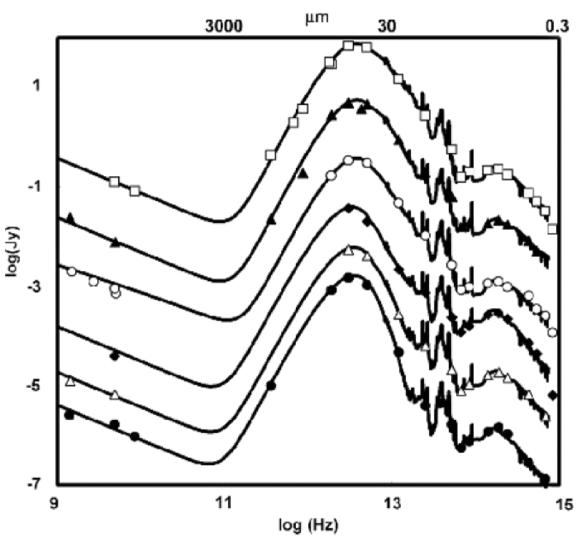
Figure 1.— Full LIRG SEDs and defining photometric points. Between 5 and 36$\mu$m the SEDs are based on IRS spectra rather than the photometry. The curves have been offset for clarity; from top to bottom the galaxies and offset factors are: 1.) NGC 1614 (2); 2.) NGC 4194 (0.2); 3.) NGC 3256 (0.003); 4.) NGC 2369 (0.001); 5.) ESO 0320-g030 (0.0001); and 6.) Zw 049.057 (0.00005).

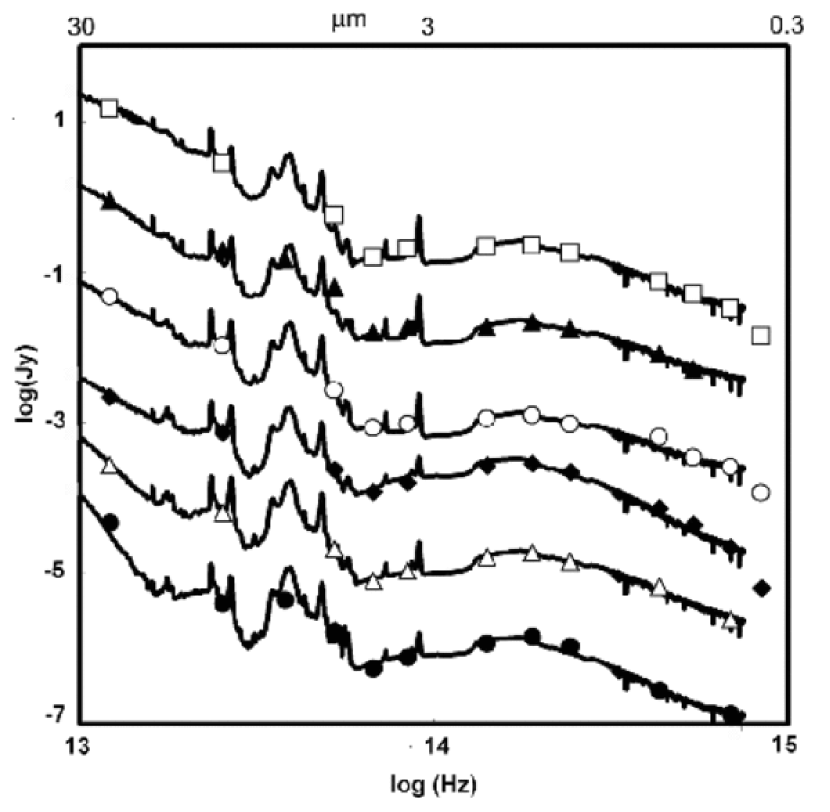
Figure 2.— Expanded LIRG SEDs to highlight optical through mid-IR. The order of galaxies and offsetting factors are as in Figure 1.

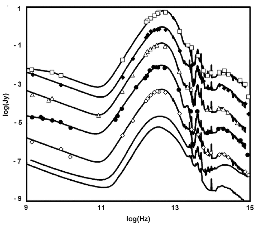
Figure 3.— Full ULIRG SEDs and defining photometric points. Between 5 and 36$\mu$m the SEDs are based on IRS spectra rather than the photometry. The curves have been offset for clarity; from top to bottom the galaxies and offset factors are: 1.) IRAS 22491-1808 (1); 2.) IRAS 14348-1447 (0.1); 3.) IRAS 17208-0018 (0.003); 4.) Arp 220 (0.00007); 5.) IRAS 12112+0305 (0.00005); 6.) Dale alpha = 1.5 model; and 7.) Chary & Elbaz L(TIR) = $2\times 10^{12}$ model.

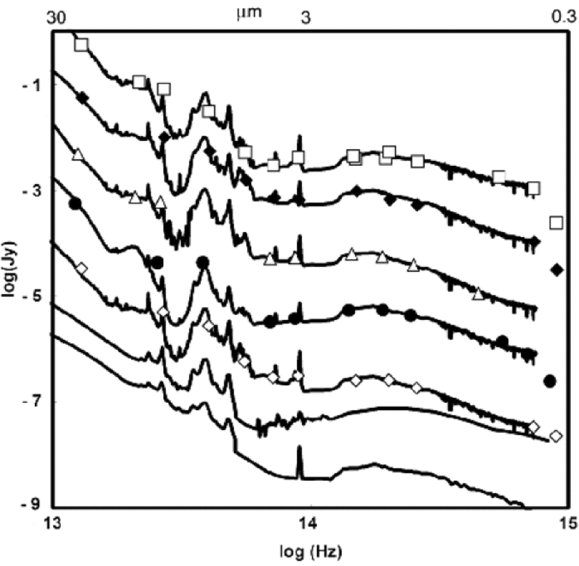
Figure 4.— Expanded ULIRG SEDs to highlight optical through mid-IR. The order of galaxies and offsetting factors are as in Figure 3.

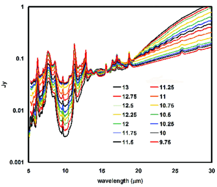
Figure 5.— Family of average spectral templates in the 5 to 37$\mu$m range. These templates are used for K-correction to 24$\mu$m rest band. The templates are keyed to the log(L(TIR)) of the galaxies, calculated as by Sanders et al. (2003). They are normalized at 14$\mu$m. The templates for the three highest luminosities are extrapolated and are likely to be significantly less representative than the rest.

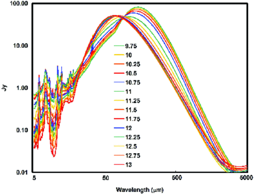
Figure 6.— Family of average templates for full radio, far-infrared, and mid-infrared spectral range. The templates are keyed to the log(L(TIR)) of the galaxies, calculated as by Sanders et al. (2003). They are normalized to the same integrated flux. The templates for the three highest luminosities are extrapolated and are likely to be significantly less representative than the rest.

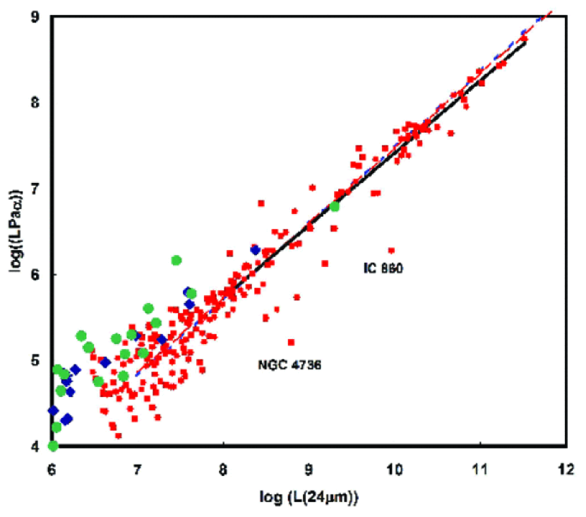
Figure 7.— Comparison of Pa$\alpha$ and 24$\mu$m luminosities. The red squares are for high metallicity galaxies and HII regions as defined by Calzetti et al. (2007); the green circles are for intermediate metallicity; and the blue diamonds are for low metallicity. The fit (black line) is to the high metallicity points. The fits to subsets of the data by Alonso-Herrero et al. (2006) and Calzetti et al. (2007) are shown as dashed red and dashed blue lines, respectively.

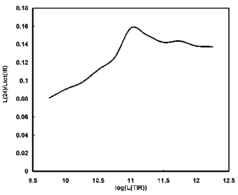
Figure 8.— Trend of L(24)/L_tot(IR) with L(TIR). L(TIR) is based strictly on the formulation of Sanders et al. (2003) using IRAS data, while L_tot(IR) is obtained by integrating under the infrared SED from 5 to 1000$\mu$m.

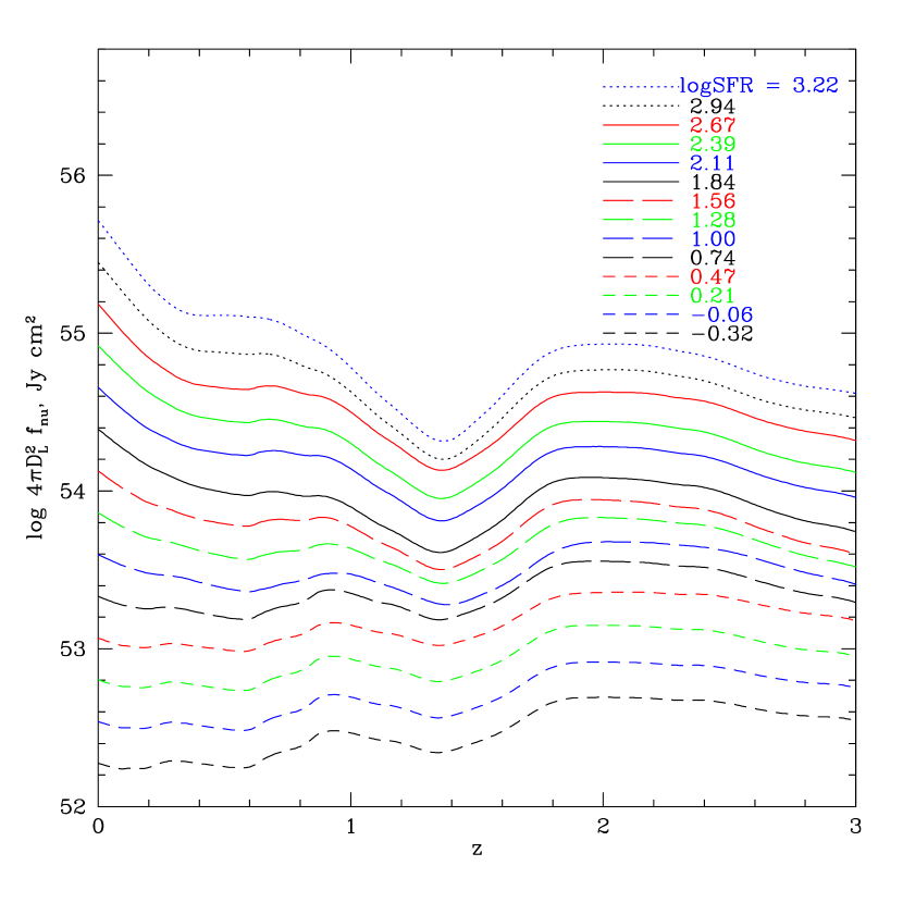
Figure 9.— Tracks of the average template SEDs vs. redshift, as would be observed at 24$\mu$m. The even spacing at any given redshift implies that a power-law fit is a good approximation to the dependence of SFR on 24$\mu$m flux.

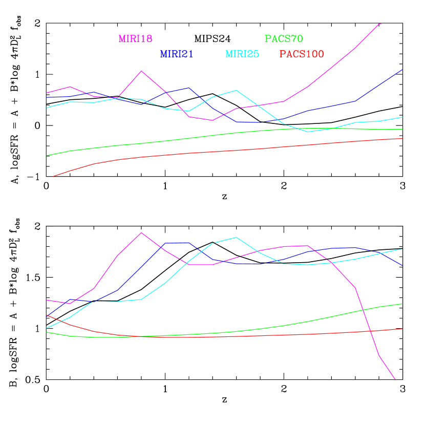
Figure 10.— Trends with redshift of the intercept $A$ and slope $B$ for the relation between SFR and infrared flux, ${\rm log~{}SFR}=A+B({\rm log}~{}4\pi D_{L}^{2}f_{\nu}\,-\,53)$, for several infrared bands: Spitzer/MIPS 24$\mu$m (heavy black line); Herschel/PACS 70 and 100$\mu$m (green and red lines); JWST/MIRI 18, 21, and 25$\mu$m (magenta, blue, and cyan lines).

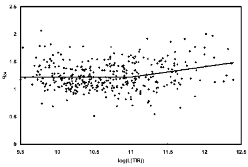
Figure 11.— Trend of q₂₄ = log[f_ν(24$\mu$m)/f$\nu$(1.4GHz)] with log(L(TIR)). The line shows our preferred fit, a constant of q₂₄=1.22 for log(L(TIR)) $<$ 11, and a sloping line above.

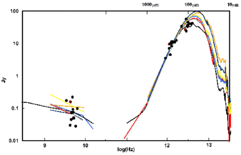
Figure 12.— Comparison of our templates with the measurements of high redshift galaxies by Kovács et al. (2006). The templates and the measurements have all been normalized near 260$\mu$m, close to the rest wavelength for the 850$\mu$m measurements of Kovács et al. (2006). There is substantial scatter in the resulting radio fluxes for the templates but even more for the radio fluxes of the high redshift galaxies. The latter are perhaps increased significantly be measurement errors (not all of which are captured in the nominal errors, as demonstrated by the results of independent reductions (Kovács et al. 2006)). Nonetheless, the local templates are very representative of the behavior of those at high redshift.

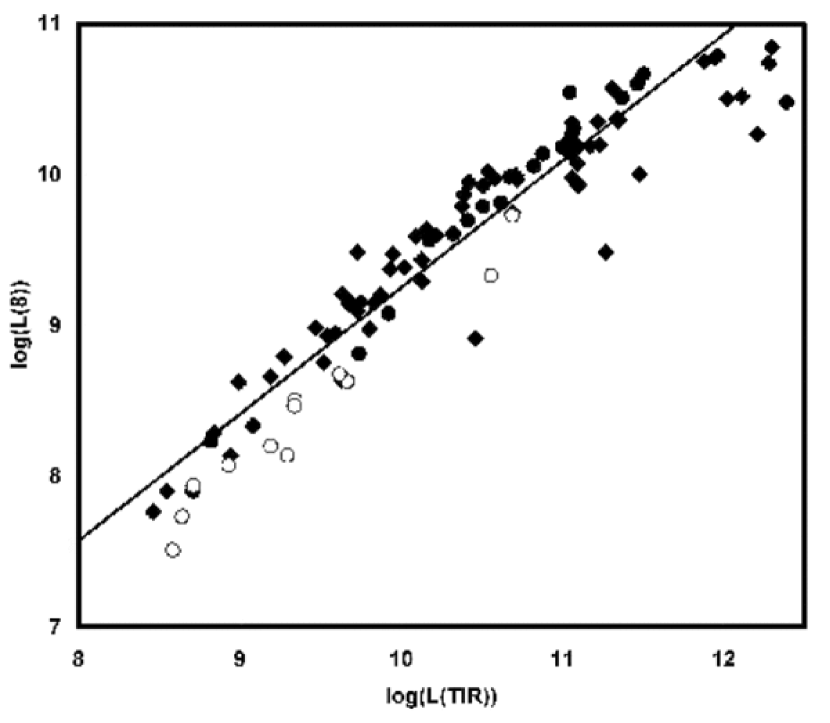
Figure 13.— Comparison of L(8) and L(TIR). Above log(L(TIR) = 11, the relation appears almost to saturate due to a number of very luminous galaxies with suppressed emission at 8$\mu$m. The diamonds are from Dale et al. (2007) and (for the LIRGs and ULIRGs) from our reduction of archival data. The circles are from Engelbracht et al. (2008); filled ones are within 0.25 dex of solar metallicity (in O/H) while open ones indicate metallicity between 0.25 and 0.5 dex below solar. The line is from Equation 21.

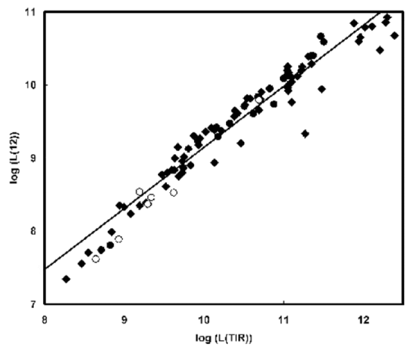
Figure 14.— Comparison of L(12) and L(TIR). The most deviant low point (NGC 1316) has been excluded from the fit. The slope is significantly different from one (see Equation 23) and there are indications of an overall curvature, with a lower ratio of L(12)/L(TIR) at high luminosity. Symbols are as for Figure 13.

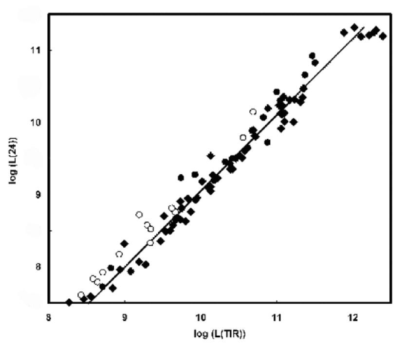
Figure 15.— Comparison of L(24) and L(TIR). The line is a linear fit as given in the text. It fits well with virtually no outliers and with a slope close to one (see Equation 25). Symbols are as for Figure 13.

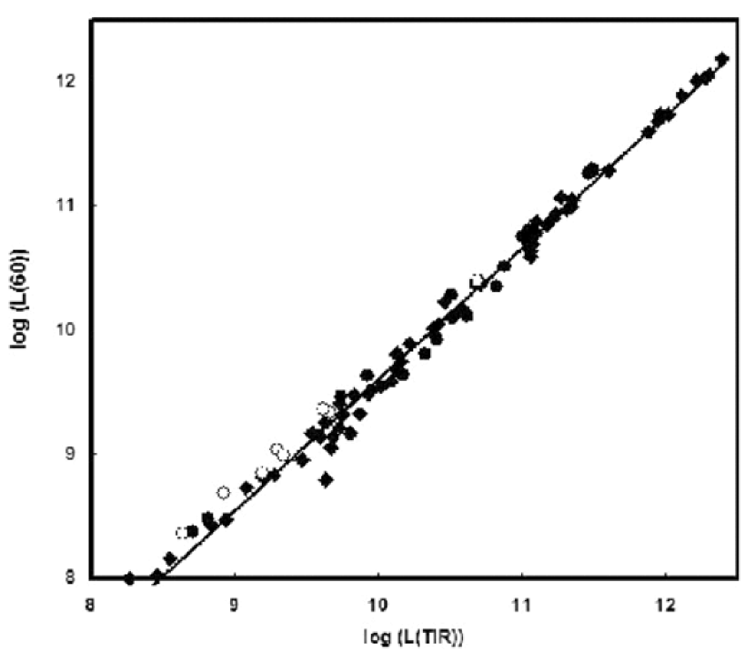
Figure 16.— Comparison of L(60) and L(TIR). The line is a linear fit given in the text. There are no outliers (not surprisingly because 60$\mu$m is close to the maximum of the SED) but the slope differs somewhat from unity (see Equation 26). Symbols are as for Figure 13.

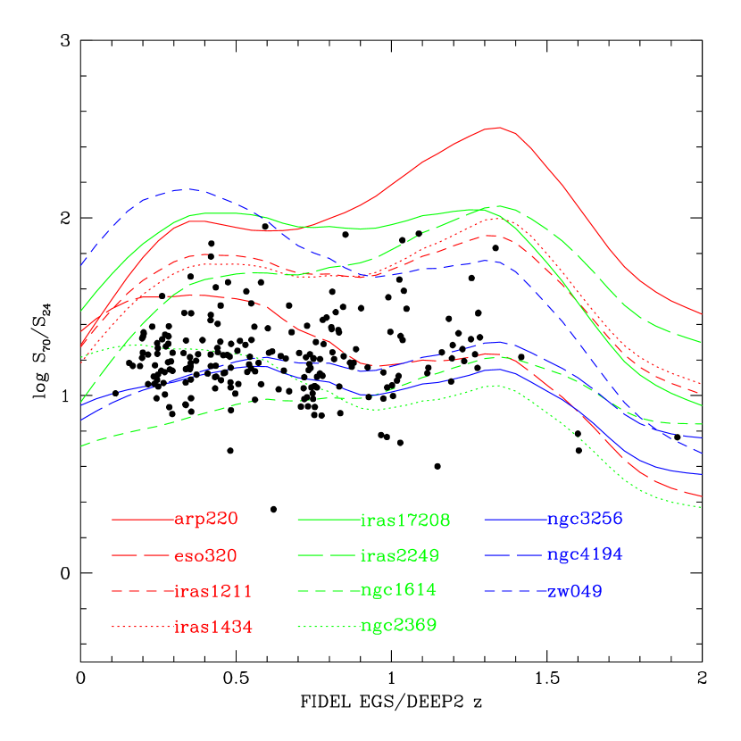
Figure 17.— Behavior of templates in the far infrared. The templates have been redshifted and convolved with the MIPS relative response functions to predict their behavior at 24 and 70$\mu$m. The points show the ratios of 70 to 24$\mu$m flux densities in the EGS/FIDEL field for galaxies with $L(TIR)>5\times 10^{9}$, and DEEP2 spectroscopic redshifts. Objects with low $S_{70}/S_{24}$ are mostly AGN. For $0<z<1$, the templates define the space occupied by the measurements well. The ”extra” template at low $z$ is Zw 49.057, which evidently represents an anomalous spectral energy distribution not seen with any significant frequency in the FIDEL data. Above z $\sim$ 1, the sensitivity limitations at 70$\mu$m should result in a substantial bias in favor of sources with large 70/24 flux ratios and against those with small ratios. Nonetheless, compared with the locus of the family of templates, few such galaxies are identified. This result supports the work of Papovich et al. (2007) and Rigby et al. (2008) that indicate an increasing relative contribution of the $\sim$ 8$\mu$m region to the total infrared outputs of galaxies at redshifts of z $\sim$ 2.

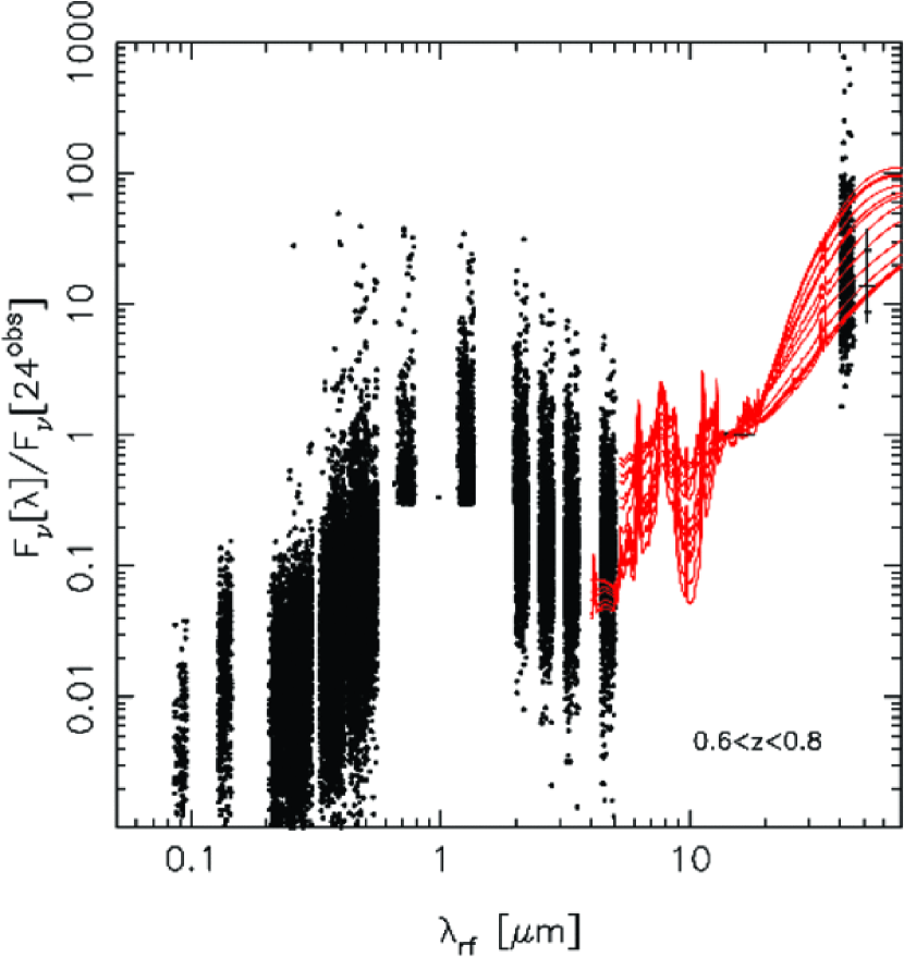
Figure 18.— Comparison of templates with photometry at z $\sim$ 0.7. The photometry is for galaxies in the EGS with [3.6] $<$ 23 (a cut that is responsible for the truncation of the distribution of points near 1 $\mu$m toward low values), photo-z between 0.6 and 0.8 (Perez-Gonzalez et al. 2008ab), a detection at 24 $\mu$m and/or 70 $\mu$m (as measured in the DR2 FIDEL data; Dickinson et al. 2007), and an estimated value of L(TIR) larger than 10¹¹ L_☉. The vertical line and marks on the right of the 70 $\mu$m fluxes show the median, quartiles and values enclosing 68% of the distribution of flux points. The templates and photometry are all normalized at observed 24$\mu$m.

References

- Alonso-Herrero et al. (2001) Alonso-Herrero, A., Engelbracht, C. W., Rieke, M. J., Rieke, G. H., & Quillen, A. C. 2001. ApJ, 546, 952
- Alonso-Herrero et al. (2006) Alonso-Herrero, A., Rieke, G. H., Rieke, M. J., Colina, L., Pérez-González, P. G., & Ryder, S. D. 2006, ApJ, 650, 835
- Alonso-Herrero et al. (2008) Alonso-Herrero, A., Rieke, G. H., Colina, L., Pereira-Santaella, M., García-Marín, M., Smith, J.-D. T., Brandl, B., Chermandaris, V., & Armus, L. 2008, submitted to ApJ
- Appleton et al. (2004) Appleton, P. N. et al. 2004, ApJS, 154, 147
- Aretxaga et al. (2005) Aretxaga, I., Hughes, D. H., & Dunlop, J. S. 2005, MNRAS, 358, 1240
- Armus et al. (2007) Armus, L. et al. 2007, ApJ, 656, 148
- Baan & Klöckner (2006) Baan, W. A. and Klöckner H.-R. 2006, A&A, 449 559
- Basu & Rana (1992) Basu, S., & Rana, N. C. 1992, ApJ, 393, 373
- Bell (2003) Bell, E. F. 2003, ApJ, 586, 794
- Beswick et al. (2008) Beswick, R. J., Muxlow, T. W. B., Thrall, H., Richards, A. M. S., & Garrington, S. T. 2008, MNRAS, 385, 1143
- Biggs & Ivison (2006) Biggs, A., & Ivison, R. J. 2006, MNRAS, 371, 963
- Biggs & Ivison (2008) Biggs, A., & Ivison, R. J. 2008, MNRAS, 385, 893
- Boyle et al. (2007) Boyle, B. J., Cornwell, T. J., Middelberg, E., Norris, R. P., Appleton, P. N., & Smail, I. 2007, MNRAS, 376, 1182
- Brandl et al. (2006) Brandl, B. R. et al. 2006, ApJ, 653, 1129
- Braun et al. (2007) Braun, R., Oosterloo, T. A., Morganti, R., Klein, U., & Beck, R. 2007, A&A, 461, 455
- Buat et al. (2007) Buat, V. et al. 2007, ApJS, 173, 404
- Calzetti et al. (2007) Calzetti, D. et al. 2007, ApJ, 666, 870
- Chabrier (2003) Chabrier, G. 2003, PASP, 115, 763
- Chapman et al. (2005) Chapman, S. C., Blain, A. W., Smail, I., & Ivison, R. J. 2005, ApJ, 622, 772
- Chary & Elbaz (2001) Chary, R., & Elbaz, D. 2001, ApJ, 556, 562
- Condon (1983) Condon, J. J. 1983, ApJS, 53, 459
- Condon et al. (1991) Condon,J. .J., Huang, Z.-P., Yin, Q. F., & Thuan, T. X. 1991, ApJ, 378, 65
- Condon et al. (1996) Condon, J. J., Helou, G., Sanders, D. B., & Soifer, B. T. 1996, ApJS, 103, 81
- Condon et al. (1998) Condon, J. J., et al. 1998, AJ, 115, 1693
- Condon et al. (2002) Condon, J. J., Cotton, W. D., & Broderick, J. J. 2002, AJ, 124, 675
- Daddi et al. (2005) Daddi, E., et al. 2005, ApJ, 631, 13
- Daddi et al. (2007) Daddi, E. et al. 2007, ApJ, 670, 156
- Dale & Helou (2002) Dale, D. A., & Helou, G. 2002, ApJ, 576, 159
- Dale et al. (2005) Dale, D. A. et al. 2005, ApJ, 633, 857
- Dale et al. (2007) Dale, D. A. et al. 2007, ApJ, 655, 863
- Davis et al. (2007) Davis, M. et al. 2007, ApJL, 660, L1
- Devereux & Eales (1989) Devereux, N. A., & Eales, S. A. 1989, ApJ, 340, 708
- Devereux et al. (1994) Devereux, N. A., Price, R., Wells, L. A., & Duric, N. 1994, AJ, 108, 1667
- Devereux et al. (1995) Devereux, N. A., Jacoby, G., Ciardullo, R. 1995, AJ, 110, 1115
- Devereux et al. (1997) Devereux, N., Duric, M., & Scowen, P. A. 1997, AJ, 113, 236
- Dickinson et al. (2007) Dickinson, M. et al. 2007, AAS, 211, 5126
- Donley et al. (2007) Donley, J. L., Rieke, G. H., Pérez-González, P. G., Rigby, J. R., & Alonso-Herrero, A. 2007, ApJ, 660, 170
- Donley et al. (2008) Donley, J. L., Rieke, G. H.,& Pérez-González, P. G., & Barro, G. 2008, ApJ, accepted
- Dopita et al. (2006) Dopita, M. A. et al. 2006, ApJ, 639, 788
- Engelbracht et al. (2007) Engelbracht, C. W. et al. 2007, PASP, 119, 994
- Engelbracht et al. (2008) Engelbracht, C. W. et al. 2008, ApJ, 678, 804
- Farrah et al. (2003) Farrah, D., Afonso, J., Efstathiou, A., Rowan-Robinson, M., Fox, M., & Clements, D. 2003,MNRAS, 343, 585
- Farrah et al. (2008) Farrah, D. et al. 2008, Astro-ph 0801.1842
- Fazio et al. (2004) Fazio, G. G. et al. 2004, ApJS, 154, 39
- Flores et al. (2004) Flores, H., Hammer, F., Elbaz, D., Cesarsky, C. J., Liang, Y. C., Fadda, D., & Gruel, N. 2004, A&A, 415, 885
- Genzel et al. (1998) Genzel, R. et al. 1998, ApJ, 498, 579
- Gibson (1998) Gibson, B. K. 1998, ApJ, 501, 675
- Gruppioni et al. (2003) Gruppioni, C. et al. 2003, MNRAS, 341, 1
- Hameed & Devereux (2005) Hameed, S., & Devereux, N. 2005, AJ, 129, 2597
- Helou et al. (1985) Helou, G., Soifer, B. T., & Rowan-Robinson, M. 1985, ApJ, 298, 7
- Hinz et al. (2004) Hinz, J. L. et al. 2004, ApJS, 154, 259
- Ho et al. (1997) Ho, L., Filippenko, A. V., & Sargent, W. L. W. 1997, ApJS, 112, 315
- Houck et al. (2004) Houck, J.R. et al. 2004,ApJS, 154, 18
- Hughes et al. (2002) Hughes, D. H., et al. 2002, MNRAS, 335, 871
- Hummer & Storey (1987) Hummer, D. G., & Storey, P. J. 1987, MNRAS, 224, 801
- Ibar et al. (2008) Ibar, E., et al. 2008, MNRAS, 386. 953
- Iglesias-Páramo et al. (2006) Iglesias-Páramo, J., et al. 2006, ApJS, 164, 38
- Iono et al. (2005) Iono, D., Yun, M.& Ho, L. 2005, ApJS, 158, 1
- Ivison et al. (2007) Ivison, R. J. et al. 2007, MNRAS, 380, 199
- Kennicutt (1998) Kennicutt, R. C. 1998, ARA&A, 36, 189
- Kennicutt et al. (2007) Kennicutt, R. C. et al. 2007, ApJ, 671, 333
- Kim et al. (1995) Kim, D.-C., Sanders, D.B., Veilleux, S., Mazzarella, J.M., & Soifer, B.T. 1995, ApJS, 98, 129
- Kim et al. (2001) Kim, D.-C., Veilleux, S., & Sanders, D. B. 2001, ApJS, 143, 277
- Kovács et al. (2006) Kovács, A., Chapman, S. C., Dowell, C. D., Blain, A. W., Ivison, R. J., Smail, I., & Phillips, T. G. 2006, ApJ, 650, 592
- Kroupa (2002) Kroupa, P. 2002, Science, 295, 82
- Kruit, van der (1971) Kruit, P. C. van der, 1971, A&A, 15, 110
- Lacy et al. (2004) Lacy, M. et al. 2004, ApJS, 154, 166
- Le Floc’h et al. (2005) Le Floc’h, E. et al. 2005, ApJ, 632, 169
- Lu et al. (2003) Lu, N. et al. 2003, ApJ, 588, 199
- Maiolino & Rieke (1995) Maiolino, R., & Rieke, G. H. 1995, ApJ, 454, 95
- Marcillac et al. (2006) Marcillac, D., Elbaz, D., Chary, R. R., Dickinson, M., Galliano, F., & Morrison, G. 2006, A&A, 451, 57
- Marleau et al. (2007) Marleau, F. R., Fadda, D., Appleton, P. N., Noriega-Crespo, A., Im, M., & Clancy, D. 2007, ApJ, 663, 218
- Miller & Scalo (1979) Miller, G. E., & Scalo, J. M. 1979, ApJS, 54, 513
- Papovich & Bell (2002) Papovich, C., & Bell, E. F. 2002, ApJ, 529, 1
- Papovich et al. (2007) Papovich, C. et al. 2007, ApJ, 668, 45
- Perez-Gonzalez et al. (2005) Pérez-González, P. G. et al. 2005, ApJ, 630, 82
- Perez-Gonzalez et al. (2008a) Pérez-González, P. G. et al. 2008a, ApJ, 675, 234
- Perez-Gonzalez et al. (2008b) Pérez-González, P. G., Trujillo, I., Barro, G., Gallego, J., Zamorano, J., Conselice, C. J. 2008b, astro-ph/0807.1069
- Pope et al. (2008) Pope, A., et al. 2008, ApJ, 675, 1171
- Popescu et al. (2002) Popescu, C. C., Tuffs, R. J., Völk, H. J., Pierini, D., & Madore, B. F. 2002, ApJ, 567, 221
- Prescott et al. (2007) Prescott, M. K. M. et al. 2007, ApJ, 668, 182
- Rieke & Lebofsky (1985) Rieke, G. H., & Lebofsky, M. J. 1985, ApJ, 288, 618
- Rieke & Lebofsky (1986) Rieke, G. H., & Lebofsky, M. J. 1986, ApJ, 304, 326
- Rieke et al. (1993) Rieke, G. H., Loken, K., Rieke, M. J. & Tamblyn, P. 1993, ApJ, 412, 99
- Rieke & Low (1972) Rieke, G. H., & Low, F. J. 1972, ApJ, 176, 95
- Rieke et al. (2004) Rieke, G. H. et al. 2004, ApJS, 154, 25
- Riffel et al. (2006) Riffel, R.,Rodriguez-Ardilla, A., & Pastorize, M. G. 2006, A&A, 457, 61
- Riffel et al. (2008) Riffel, R., Pastoriza, M. G., Rodríguez-Ardila, A., & Maraston, C. 2008, astro-ph 0805.1167
- Rigby & Rieke (2004) Rigby, J. R., & Rieke, G. H. 2004, ApJ, 606, 237
- Rigby et al. (2007) Rigby, J. R. et al. 2008, ApJ, 675, 262
- Rigopoulou et al. (1999) Rigopoulou, D., Spoon, H. W. W., Genzel,R., Lutz, D., Moorwood, A. F. M., & Tran, Q. D. 1999, AJ, 118, 2625
- Roussel et al. (2001) Roussel, H., Sauvage, M., Vigroux, L. & Bosma, A. 2001, A&A, 372, 427
- Roy et al. (2008) Roy, A. L., Goss, W. M., & Anantharamaiah, K. R. 2008, A&A, 483, 79
- Sajina et al. (2007) Sajina, A., Yan, L., Armus, L., Choi, P., Fadda, D., Helou, G.,& Spoon, H. 2007, ApJ, 664, 713
- Sakamoto et al. (2008) Sakamoto, K. et al. 2008, Astro-ph 0806.0217
- Sanders et al. (2003) Sanders, D. B., Mazzarella, J. M., Kim, D.-C., Surace, J. A, & Soifer, B. T. 2003, AJ, 126, 1607
- Sanders & Mirabel (1996) Sanders, D. B., & Mirabel, I. F. 1996, ARA&A, 34, 749
- Schmitt et al. (2006) Schmitt, H. R. et al. 2006, ApJ, 643, 173
- Seymour et al. (2008) Seymour, N. et al. 2008, MNRAS, 386, 1695
- Siebenmorgen & Krügel (2007) Siebenmorgen,R. & Krügel, E. 2007, A&A, 461, 445
- Smith et al. (2007) Smith, J. D. et al. 2007, ApJ, 656, 770.
- Stern et al. (2005) Stern, D. et al. 2005, ApJ, 631, 163
- Sturm et al. (2000) Stürm, E., Lutz, D., Tran, D., Feuchtgruber, H., Genzel, R., Kunze, D., Moorwood, A. F. M., & Thornley, M. D. 2000, A&A, 358, 481
- Strecker et al. (1979) Strecker, D. W., Erickson, E. F., & Witteborn, F. C. 1979, ApJS, 41, 501
- Sullivan et al. (2003) Sullivan, M., Mobasher, B., Chan, B., Cram, L., Ellis, R., Treyer, M., & Hopkins, A. 2001, ApJ, 558, 72
- Surace & Sanders (2000) Surace, J. A., & Sanders, D. B. 2000, AJ, 120, 604
- Taylor et al. (2005) Taylor, V. A., Jansen, R., Windhorst, R. A., Odewahn, S. C.,& Hibbard, J. E. 2005, ApJ, 630, 784
- Tabatabaei et al. (2007) Tabatabaei, F. S. et al. 2007, A&A, 466, 509
- Tacconi et al. (2006) Tacconi, L. J. et al. 2006, ApJ, 640, 228
- Taniguchi et al. (1996) Taniguchi, Y., Ohyama, Y., Yamada, T., Mouri, H., & Yoshida, M. 1996, ApJ, 467, 215
- Veilleux et al. (1995) Veilleux, S., Kim, D.-C., Sanders, D. B., Mazzarella, J. M., & Soifer, B. T. 1995, ApJS, 98, 171
- Vlahakis et al. (2007) Vlahakis, C., Eales, S., & Dunne, L. 2007, MNRAS, 379, 1042
- Walker et al. (1988) Walker, C.E., Lebofsky, M.J., & Rieke, G.H. 1988, ApJ, 325, 687
- Wang & Heckman (1996) Wang, B., & Heckman, T.M. 1996, ApJ, 457, 645
- Wang & Silk (1993) Wang, B., & Silk, J. 1993, ApJ, 406, 580
- White & Becker (1992) White, R. L., & Becker, R. H. 1992, ApJS, 79, 331
- Younger et al. (2008) Younger, J. D. et al. 2008, Astro-ph 0807.2243
- Yun et al. (2001) Yun, M. S., Reddy, N. A., & Condon, J. J. 2001, ApJ, 554, 803