Modeling Molecular Hydrogen and Star Formation in Cosmological Simulations

Abstract

We describe a phenomenological model for molecular hydrogen formation suited for applications in galaxy formation simulations, which includes non-equilibrium formation of H₂ on dust and approximate treatment of both its self-shielding and shielding by dust from the dissociating UV radiation. The model is applicable in simulations in which individual star forming regions – the giant molecular complexes – can be identified (resolution of tens of pc) and their mean internal density estimated reliably, even if internal structure is not resolved. In agreement with previous studies, calculations based on our model show that the transition from atomic to fully molecular phase depends primarily on the metallicity, which we assume is directly related to the dust abundance, and clumpiness of the interstellar medium. The clumpiness simply boosts the formation rate of molecular hydrogen, while dust serves both as a catalyst of H₂ formation and as an additional shielding from dissociating UV radiation. The upshot is that it is difficult to form fully-shielded giant molecular clouds while gas metallicity is low. However, once the gas is enriched to $Z\sim 0.01-0.1Z_{\odot}$, the subsequent star formation and enrichment can proceed at a much faster rate. This may keep star formation efficiency in the low-mass, low-metallicity progenitors of galaxies very low for a certain period of time with the effect similar to a strong “feedback” mechanism. The effect may help explain the steep increase of the mass-to-light ratio towards smaller masses observed in the local galaxy population. We apply the model and star formation recipes based on the local amount of molecular gas to an output from a cosmological simulation of galaxy formation and show that resulting global correlations between star formation and gas and H₂ surface densities are in good agreement with observations.

1. Introduction

Detailed understanding of galaxy formation remains one of the most important goals of modern astrophysics. A critical challenge for achieving this goal, in addition to a sheer variety of physical processes and the range of spatial and temporal scales involved, is our poor understanding of how gas is converted into stars under different conditions. This conversion controls critical aspects of the final galaxy properties from its total stellar mass and star formation history to its morphology, which depends on the relative timing of gas conversion to stars and the epoch of major mergers and rapid mass assembly.

Recent observational and theoretical progress in understanding star formation on the scale of molecular clouds points towards a prescription for star formation on larger, galactic scales. In particular, the observational data support the theoretically motivated view of molecular clouds in which the specific star formation rate per local free fall time in the molecular gas is essentially independent of the local gas density (Krumholz & McKee, 2005; Krumholz & Tan, 2007a; Krumholz et al., 2008a). This is fortunate because the efficiency of star formation can then be modeled in a simulation as long as (i) one can resolve and identify the regions corresponding to star forming molecular clouds in a simulation and (ii) achieve resolution sufficient to model their mean internal density properly.

Until recently, these conditions were not easily achievable in cosmological simulations due to numerical limitations on spatial and mass resolution. The standard approach in galaxy formation modeling so far (c.f. recent studies by Brooks et al., 2007; Governato et al., 2007; Ceverino & Klypin, 2007; Scannapieco et al., 2008; Croft et al., 2008; Oppenheimer & Davé, 2008; Tasker & Bryan, 2008; Mayer et al., 2008, and many earlier works, comprehensively reviewed in the last reference) was to adopt a recipe which ties the local star formation rate density to the gas density via a universal relation, often with threshold conditions on the gas properties (density, temperature, etc). Such recipes are loosely based on the empirical correlations observed for local galaxies (the Kennicutt-Schmidt, hereafter KS, relations: Schmidt, 1959, 1963; Kennicutt, 1989, 1998b). However, these relations have only been studied relatively well for nearby massive or star bursting galaxies. There is, however, a growing body of evidence that the relations for galaxies of lower surface brightness and/or metallicity may be quite different (see, e.g., Robertson & Kravtsov, 2008, for references and discussion and the recent study by Bigiel et al. 2008).

Indeed, as we emphasize below (see also Elmegreen, 1989, 1993; Schaye, 2001; Pelupessy et al., 2006; Krumholz et al., 2008b), the transition from atomic to fully molecular gas depends strongly on the local gas metallicity and dissociating UV flux. Thus, for example, we expect that in low metallicity galaxies gas becomes fully molecular (and thereby conducive to star formation) at higher gas density compared to more massive, higher metallicity systems. This means that on the global scale of a galaxy gas may be converted into stars at a slower rate per unit mass of gas or, in other words, the star formation efficiency is lower, even if the density distribution of ISM is the same. Not only is this regime applicable to dwarf or low surface brightness galaxies today, but also to the majority of progenitors of massive galaxies at high redshifts.

The lower efficiency of gas conversion into stars at high redshifts may have profound implications for galaxy evolution from shaping the faint end of the luminosity function to the morphological mix of galaxies. Traditionally, in cosmological simulations and semi-analytic models the efficiency of star formation in $\lesssim L_{\ast}$ galaxies is suppressed by supernova feedback. However, the efficiency of such suppression is not clear and in many observed dwarf galaxies star formation is inefficient without obvious signs of active feedback. We argue that a similar suppression can be provided by the inherent difficulty of building self-shielding molecular regions within low-density, low-metallicity ISM of smaller galaxies.

Current self-consistent cosmological simulations of galaxy formation can resolve scales of molecular clouds (i.e., tens of parsecs, Kravtsov, 2003; Ceverino & Klypin, 2007; Tasker & Bryan, 2008; Razoumov, 2008; Gibson et al., 2008) and can, therefore, explore the effect of ISM process on the efficiency of star formation self-consistently. Observational evidence for the universal efficiency of gas conversion per free fall time in molecular clouds can then be adopted as a well-motivated and robust star formation prescription, even if the internal density structure of the star forming regions is not well resolved. Such recipe is promising but requires a model for the formation and destruction of molecular gas in the simulations in order to correctly identify the regions of current star formation.

Several such models have recently been developed and implemented in the SPH simulations (Pelupessy et al., 2006; Booth et al., 2007; Robertson & Kravtsov, 2008). Pelupessy et al. (2006) have followed reactions of H₂ formation and destruction, following reactions of H₂ formation on dust grains and dust and self-shielding from UV radiation and using a sub-grid model for gas clouds, which uses observed cloud scaling relations. One of the main conclusions of their study was the strong dependence of the molecular gas fraction on the ambient metallicity of ISM. Booth et al. (2007) have adopted a different approach, in which they model formation of molecular clouds using a model based on collisions between clouds representing molecular clouds as ballistic particles coagulating upon collision. They have demonstrated that with such a model many observed properties of disc galaxies can be reproduced. Recently, Robertson & Kravtsov (2008) presented a model of star formation based on the local molecular gas content. The latter was modeled by using pre-computed tables of molecular fraction as a function of local gas properties (density, temperature, metallicity and UV flux). The authors showed that the model implied a significant steepening of the Kennicutt-Schmidt relations in low surface density, low molecular fraction environments characteristic of dwarf and low surface brightness galaxies, as well as of the outskirts of disks in larger galaxies. This study has indicated that one of the key factors controlling the amount of diffuse molecular gas in the lower density ISM is UV radiation from the recent local star formation.

In this paper we present a model of molecular gas evolution and H₂-based star formation together with their implementation in the Adaptive Refinement Tree (ART) code for cosmological simulations. The ART code is a Eulerian hydrodynamics$+N$-body code, which uses Adaptive Mesh Refinement (AMR) technique to reach high resolution in the regions of interest (i.e., in high-density regions of ISM in the case of this study). We present details of the model of molecular hydrogen formation and disruption and test the model against available observations. We discuss several star formation recipes for the gas conversion in molecular clouds and present resulting Kennicutt relations, when such recipes and the molecular hydrogen model are applied to a realistic cosmological simulation of a Milky Way progenitor. In a follow-up study, we plan to explore the differences of such model compared to the old star formation prescriptions in full cosmological simulations.

2. Method

2.1. Description of Simulations

The cosmological simulation used as a testing ground for our model for molecular hydrogen formation has been described in detail in Tassis et al. (2008) as a run “FNEC-RT”. Here we only recap that the simulation was performed with the Eulerian, gas dynamics + $N$-body Adaptive Refinement Tree (ART) code (Kravtsov et al., 1997; Kravtsov, 1999; Kravtsov et al., 2002), which uses adaptive mesh refinement (AMR) in both the gas dynamics and gravity calculations to achieve a needed dynamic range.

The simulation follows a Lagrangian region corresponding to five virial radii of a system, which evolves to approximately Milky Way mass ($M\approx 10^{12}{\rm\ M_{\odot}}$) at $z=0$. The mass resolution in dark matter of $m_{\rm dm}=1.3\times 10^{6}\mbox{\,M}_{\odot}$ (and corresponding resolution in gas dynamics of $m_{\rm gas}=2.2\times 10^{5}\mbox{\,M}_{\odot}$). This Lagrangian region is embedded into a cubic volume of $6h^{-1}$ comoving Mpc on a side, which is resolved to a lesser extent throughout the simulation.

The simulation includes star formation and supernova enrichment and energy feedback, and uses self-consistent 3-D radiative transfer of UV radiation from individual stellar particles using the OTVET approximation (Gnedin & Abel, 2001). The simulation follows non-equilibrium chemical network of hydrogen and helium and non-equilibrium cooling and heating rates, which make use of the local abundance of atomic, molecular, and ionic species and UV intensity, followed self-consistently during the course of the simulation. We use the $z=4$ output of the simulation as at this epoch the gaseous disk of the main galaxy is relatively quiescent and has not experienced major mergers since $z\approx 6$.

A new ingredient in the simulation, beyond what has been described in Tassis et al. (2008), is an empirical model for formation and shielding of molecular hydrogen on the interstellar dust, which is described in the following section.

2.2. The model for tracking molecular hydrogen

The two key processes controlling the abundance of molecular gas in the ISM enriched with metals are the formation of ${{\rm H}_{2}}$ on dust grains and its shielding from photodissociation by the interstellar radiation field by itself (self-shielding) and by dust (see Glover & Mac Low, 2007, for a recent review and references to a large body of prior work).

Unfortunately, the exact treatment of shielding cannot be achieved in modern cosmological simulations, as it requires three-dimensional radiative transfer, including radiative transfer in the Lyman-Werner bands. Therefore, we adopt a phenomenological treatment of molecular hydrogen shielding, which is tuned to reproduce available observations (see below).

In the optically thin regime (no shielding) and in the absence of dust, equations for the balance of neutral (atomic) hydrogen and molecular hydrogen can be written as

$$\dot{X}_{{\rm H\,I}} = R(T)n_{e}X_{{\rm H\,II}}-X_{{\rm H\,I}}\Gamma_{{\rm H\,I}}-2\dot{X}_{{{\rm H}_{2}}},$$

$$\dot{X}_{{{\rm H}_{2}}} = \dot{X}_{{{\rm H}_{2}}}^{\rm gp},$$ (1)

where $X_{i}$ denotes a number fraction of baryons in species $i$,

$$X_{i}\equiv n_{i}/n_{b},$$

and $n_{b}$ is the total number density of baryons. In equations (1) $R(T)$ is the recombination rate, $n_{e}$ is the number density of free electrons, $\Gamma_{HI}$ is the hydrogen ionization rate, and the term $\dot{X}_{{{\rm H}_{2}}}^{\rm gp}$ includes multiple processes of formation and destruction of molecular hydrogen in the gas phase reactions, via ${\rm H}^{-}$ and ${{\rm H}_{2}}^{+}$ ions. The latter reactions are comprehensively summarized elsewhere (Shapiro & Kang, 1987; Abel et al., 1997; Galli & Palla, 1998; Glover & Jappsen, 2007; Glover & Abel, 2008) and are not important for our purposes; we keep them in the equations to ensure that our model also works in the metal-free regime.

Physically, the effect of the geometric shielding by dust grains and ${{\rm H}_{2}}$ self-shielding can be described by effective shielding factors, $S_{d}$ and $S_{{\rm H}_{2}}$, which take values from 0 to 1. Incorporating these factors, and adding molecular hydrogen formation on dust, equations (1) become

$$\dot{X}_{{\rm H\,I}} = R(T)n_{e}X_{{\rm H\,II}}-S_{d}X_{{\rm H\,I}}\Gamma_{{\rm H\,I}}-2\dot{X}_{{{\rm H}_{2}}},$$

$$\dot{X}_{{{\rm H}_{2}}} = S_{d}S_{{\rm H}_{2}}\dot{X}_{{{\rm H}_{2}}}^{\rm gp}+R_{d}n_{b}X_{\rm H\,I}\left(X_{\rm H\,I}+2X_{{\rm H}_{2}}\right),$$ (2)

where we assume that the dust absorption also affects atomic hydrogen ionization rate. In principle, this is not a crucial assumption since one would expect that hydrogen is predominantly neutral in regions where dust absorption is important. In practice, however, the OTVET approximation for modeling radiative transfer, which we use in our simulations, is somewhat diffusive. In simulations presented here, this diffusion leads to ionizing radiation leaking into neutral, self-shielded gas. The numerical diffusion effect is not significant, but introducing a factor $S_{d}$ in equation (2a) allows to essentially eliminate it altogether. In a completely analogous manner, we also reduce the photo-heating rate of the gas in the evolution equation for the gas internal energy.

The specific form of the shielding factors $S_{d}$ and $S_{{\rm H}_{2}}$ cannot be computed without a detailed treatment of radiative transfer in the Lyman-Werner bands. Our goal, therefore, is to find physically plausible functional forms that are motivated by the observational data. To this end, we follow Draine & Bertoldi (1996, see also ) and define these two factors as

$$S_{d}=e^{\displaystyle-\sigma_{d,\rm eff}(N_{\rm H\,I}+2N_{{\rm H}_{2}})}$$

and

$$S_{{\rm H}_{2}}=\frac{1-\omega_{{\rm H}_{2}}}{(1+x)^{2}}+\frac{\omega_{{\rm H}_{2}}}{(1+x)^{1/2}}e^{\displaystyle-0.00085(1+x)^{1/2}},$$

where $x\equiv N_{{\rm H}_{2}}/(5\times 10^{14}\mbox{\,cm}^{2})$ and $\sigma_{d,\rm eff}$ and $\omega_{{\rm H}_{2}}$ are treated as adjustable parameters. We find that we obtain the best fit with the observational data (as we demonstrate below) for values of these parameters $\sigma_{d,\rm eff}=4\times 10^{-21}\mbox{\,cm}^{2}$ and $\omega_{{\rm H}_{2}}=0.2$, which are slightly different from those adopted by Glover & Mac Low (2007).

The formation rate coefficient of molecular hydrogen on dust, $R_{d}$, has been studied extensively in the past. While reviewing comprehensively this large body of work is beyond the scope of this paper, we would like to note that a theoretically calculated formula from Hollenbach & McKee (1979) and Burke & Hollenbach (1983) has been most commonly used in the past (see Cazaux & Spaans, 2004, for a recent review). In this work, following our main ideology of using the most empirically determined quantities, we adopt an observationally determined value for $R_{d}$ from Wolfire et al. (2008). We also assume that the dust-to-gas ratio scales linearly with gas metallicity $Z$ (in solar units) and that the gas is clustered on scales unresolved in our simulations, so that the effective ${{\rm H}_{2}}$ formation rate is higher in proportion to the gas clumping factor, $C_{\rho}\equiv\langle\rho^{2}\rangle/\langle\rho\rangle^{2}$,

$$R_{d}=3.5\times 10^{-17}ZC_{\rho}\mbox{\,cm}^{3}/\mbox{\,s}.$$ (3)

The clumping factor $C_{\rho}$ can be viewed as a parameter of our model. However, there is also some theoretical arguments for its plausible range of values. Numerical simulations of turbulent molecular clouds typically find a lognormal density distribution inside the clouds with the width that depends on the average Mach number of the flows: $\sigma_{\ln\rho}^{2}\approx 1-2$ (Padoan et al., 1997; Ostriker et al., 2001; McKee & Ostriker, 2007). Since for a lognormal distribution,

$$C_{\rho}=e^{\displaystyle\sigma_{\ln\rho}^{2}},$$

most likely values for the clumping factor are in the range $C_{\rho}\sim 3-10$. Empirical evidence also indicates that gas in molecular clouds is highly clumped with the ratio of typical molecular gas density to the mean cloud density of $\sim 30-100$ (see §3.1.2 in McKee & Ostriker, 2007, and references therein).

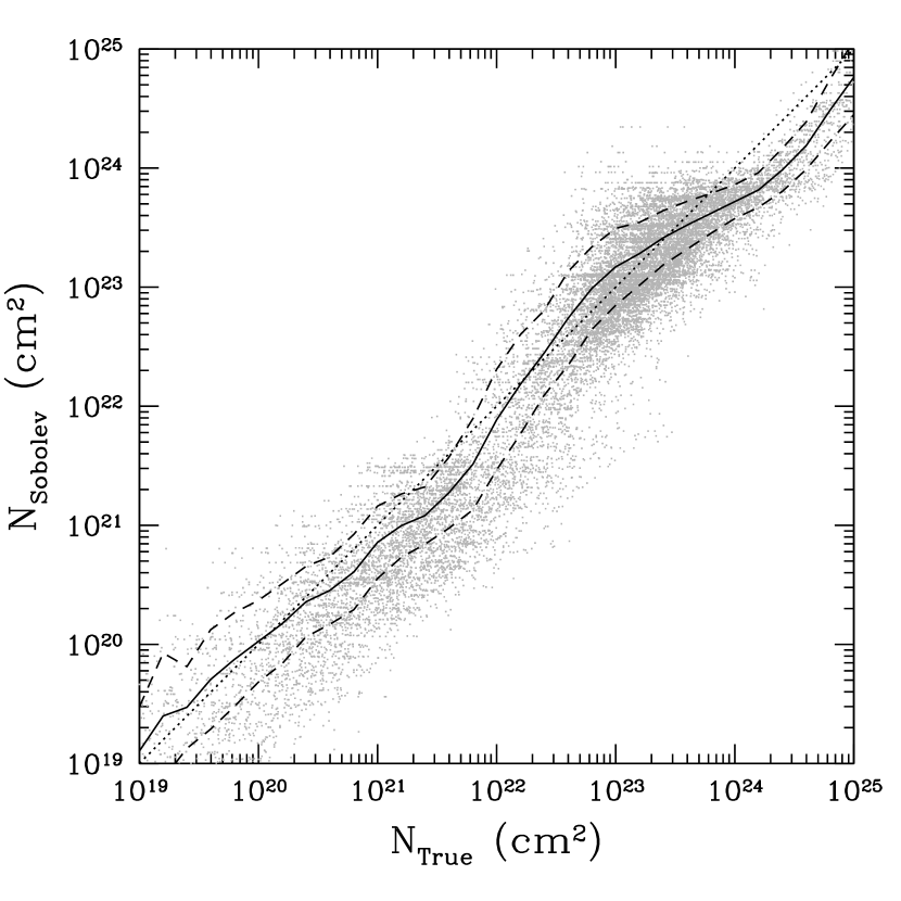
Figure 1.— Comparison of the total hydrogen column density from the Sobolev-like approximation and the true column density as integrated along random lines of sight through the simulation box. Gray points show individual lines of sight; black solid line show the average $N_{\rm Sobolev}$ for a given $N_{\rm True}$, while black dashed lines give the rms scatter. The thin black dotted line is a diagonal of the plot.

Finally, in order to specify the column densities inside the molecular clouds, we use a Sobolev-like approximation:

$$N_{i}\approx n_{i}L_{\rm Sob},$$ (4)

where

$$L_{\rm Sob}\equiv\frac{\rho}{\left|\nabla\rho\right|}.$$

We have verified that equation (4) provides an essentially unbiased estimate for the true column density (obtained by integrating along random lines of sight) within the range $3\times 10^{20}\mbox{\,cm}^{2}<N_{\rm H\,I}+2N_{{\rm H}_{2}}<3\times 10^{23}\mbox{\,cm}^{2}$ with a scatter of about a factor of 2, as illustrated in Figure 1.

In the gas dynamics solver and in the calculation of the cooling function, we use the thermodynamically correct relations between the gas internal energy, pressure, and temperature, without assuming a polytropic approximation, which becomes invalid for mostly molecular gas (Turk, Gnedin, & Abel, in preparation).

This model is implemented in the ART code. Because individual molecular clouds are not resolved in our simulations, the specific numerical implementation suffers from numerical artifacts due to finite spatial resolution. We discuss these artifacts and our approach for their mitigation in the Appendix.

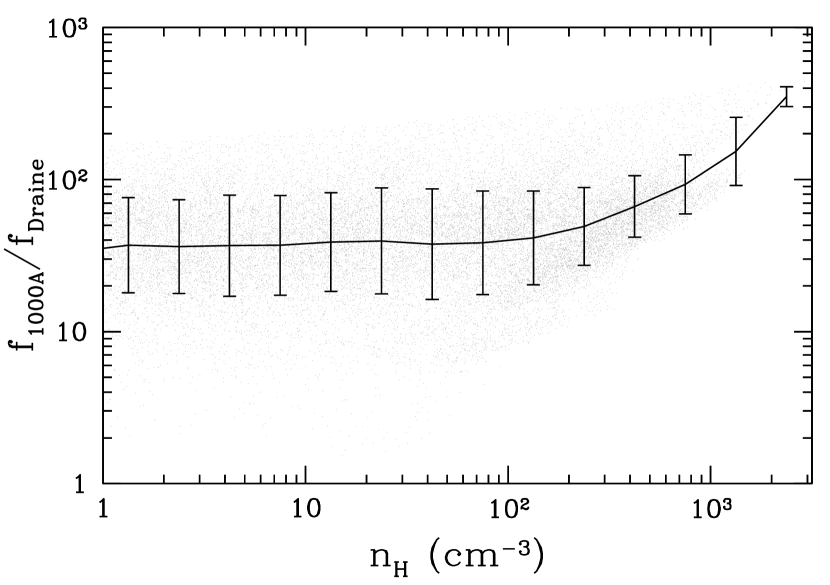
Figure 2.— The intensity of the interstellar radiation field at $1000\AA$ as a function of gas density in the parent simulation FNEC-RT, in units of the Draine (1978) field ($10^{6}\mbox{\,photons}/\mbox{\,cm}^{2}/\mbox{\,s}/\mbox{\,sterrad}/\mbox{\,eV}$). Since the parent simulation does not include dust shielding, radiation at $1000\AA$ in that simulation was computed in the optically thin regime.

2.3. Star Formation

We explore three simple star formation recipes, based on the local density of molecular hydrogen, in order to test the dependence of global KS relations on the underlying assumptions. We can write the star formation rate in a molecular cloud in terms of an efficiency factor $\epsilon$, equivalent to the inverse of the (molecular) gas consumption timescale, as

$$\dot{\rho}_{\star}=\epsilon\rho_{{{\rm H}_{2}}},$$ (5)

where $\dot{\rho}_{\star}$ is the star formation rate per unit volume, and $\rho_{{{\rm H}_{2}}}$ is the molecular hydrogen density. We can then express $\epsilon$ in terms of a dimensionless effective efficiency $\varepsilon_{\rm ff}$ per local free-fall time of the gas, so that

$$\dot{\rho}_{\star}=\frac{\varepsilon_{\rm ff}}{\tau_{\rm sf}}\rho_{{{\rm H}_{2}}},$$ (6)

where $\tau_{\rm sf}=\tau_{\rm ff}=\sqrt{3\pi/32G\rho}$ for a uniform sphere. Since stars form out of regions of molecular complexes with sizes not necessarily resolved in our simulations, the choice of a relevant star formation timescale relies on assumption about the structure of the gas in sub-grid scales. We have tried two different assumptions about $\tau_{\rm sf}$:

SF1

the constant time scale $\tau_{\rm sf}=\tau_{\rm ff}(100\mbox{\,cm}^{-3})$, assuming all ${{\rm H}_{2}}$ in a grid cell resides in molecular clouds of average density $\approx 100\mbox{\,cm}^{-3}$;

SF2

the time scale, which depends on the cell’s gas density with an upper limit $\tau_{\rm sf}=\min[\tau_{\rm ff}(100\mbox{\,cm}^{-3}),\tau_{\rm ff}(\rho_{g,cell})]$.

SF3

the time scale, which simply depends on the density of the cell $\tau_{\rm sf}=\tau_{\rm ff}(\rho_{g,cell})$ (this recipe is similar to the one used by Robertson & Kravtsov (2008) in their models of isolated galaxies).

We adopt $\epsilon_{\rm ff}=0.01$ (Krumholz & Tan, 2007b) in all of the calculations presented below; we also use a molecular fraction threshold for computational efficiency: star formation is allowed only in cells which have a molecular fraction higher than $f_{{{\rm H}_{2}}}=0.1$. The latter criterion has a negligible impact on the total star formation rate in a galaxy, but is highly beneficial from a computational point of view, avoiding formation of a large number of very small stellar particles in low density regions.

3. Results

In this section we present results illustrating the dependence of the relative atomic and molecular gas abundances on metallicity, gas clumpiness, and UV flux. We also explore the correspondent dependencies of the global Kennicutt-Schmidt relations with different local star formation prescriptions described in the previous section.

Table 1Simulations

Simulation	Metallicity	Clumping	UV flux	SF
	$Z/Z_{\odot}$	Factor $C_{\rho}$		Recipe
A	$1$	$10$	$1$	SF2
B1	$0.3$	$10$	$1$	SF2
B2	$0.1$	$10$	$1$	SF2
C1	$1$	$1$	$1$	SF2
C2	$1$	$100$	$1$	SF2
D	$1$	$10$	$10$	SF2
E	$1$	$10$	$1$	SF1

Using the $z=4$ output of the parent FNEC-RT simulation of Tassis et al. (2008) (see § 2.1) as initial condition, we run a simulation with the model for molecular hydrogen and star formation for $100\mbox{\,Myrs}$. The baseline simulation FNEC-RT does not incorporate shielding of molecular hydrogen, and thus no molecular clouds form in that simulation. The chosen interval of time of $100\mbox{\,Myr}$ is considerably longer than the characteristic lifetime of molecular clouds ($\sim 10^{7}$ yrs, Blitz & Shu, 1980; Blitz et al., 2007) and is therefore sufficiently long for our purposes. We have also verified that our results have converged: various distribution presented below are virtually indistinguishable if we chose a $50\mbox{\,Myr}$ time interval instead.

The baseline simulation FNEC-RT also includes effects of both energy and metal feedback to the interstellar medium, to keep the tests clean both forms of feedback are turned off and the interstellar medium metallicity is kept at a constant value after our test simulation is started.

In our fiducial simulation (A) the metallicity is kept constant at solar value, we use a clumping factor $C_{p}=10$, and the star formation recipe used is SF2. The UV flux is taken directly from the parent simulation FNEC-RT and is shown in Figure 2. Our model galaxy has a significantly higher star formation rate and is smaller at $z=4$ galaxy than the Milky Way today, so the interstellar radiation field is substantially higher than the canonical Draine (1978) value adopted for the Milky Way ISM at the present time, but is consistent with the estimates of the interstellar UV field in high redshift galaxies (Chen et al., 2008).

In each of the simulations used in our parameter study, we vary a single parameter away from its fiducial simulation value. Table 1 describes the values of these free parameters in each of the simulations discussed in this section.

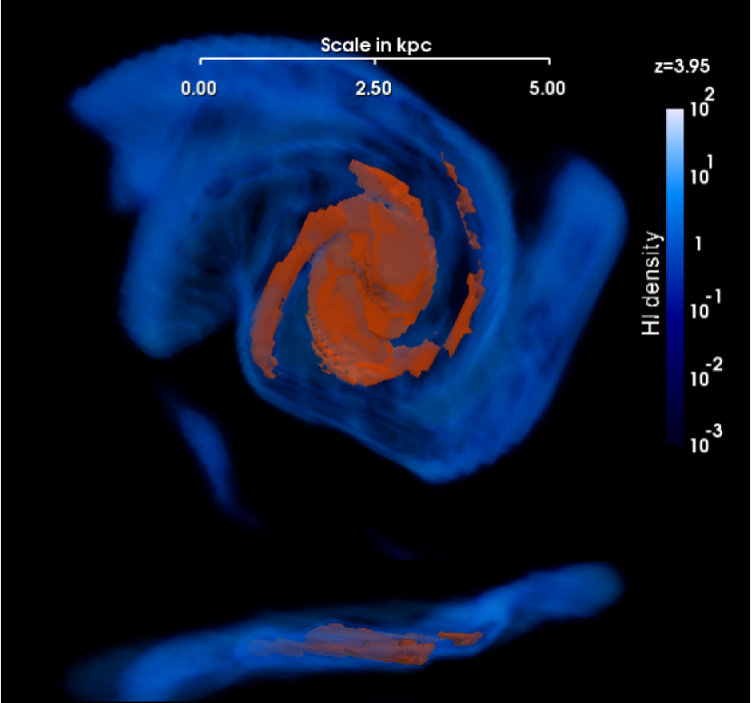
Figure 3.— A face- and edge-on views of the largest galaxy in our fiducial simulation A. Blue translucent color represents volume rendering of atomic hydrogen density, while orange color shows the location of the molecular gas (as the isosurface of $f_{{\rm H}_{2}}=0.5$ value). This figure is best viewed in color.

A visual representation of our fiducial simulation A is shown in Figure 3. The molecular gas traces spiral arms well, which are less pronounced in the atomic gas. The molecular disk is both smaller and thinner than the atomic disk. However, since our spatial resolution is only $50\mbox{\,pc}$, we do not resolve individual molecular clouds. Instead, the orange colored surface in the image shows the boundary of the mostly molecular ($f_{{\rm H}_{2}}>0.5$) gas.

3.1. Gas phases and atomic-to-molecular transition in the ISM of model galaxies

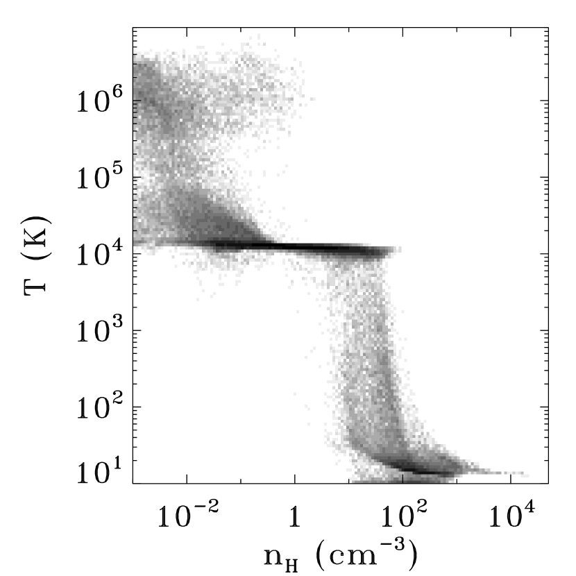
Figure 4.— Temperature plotted against the total gas number volume density for all maximum refinement level (level 9) cells at $z=4$, for simulation A.

Figure 4 shows the temperature in degrees Kelvin plotted against the total volume number density of neutral hydrogen for our fiducial simulation (A). Points in this and subsequent plots in this subsection show cells at the highest resolution level (level 9; the physical size of 52 pc at $z=4$), which cover the large fraction of the disks of galaxies forming in the high-resolution Lagrangian region of the simulation. This plot clearly shows a well developed multi-phase structure of the ISM in these disks. In particular, three different gas phases are evident: (i) the hot, ionized, low-density gas in the upper left part of the diagram; (ii) the warm neutral medium around $T\sim 10^{4}\mbox{\,K}$ and $n_{\rm H}\sim 0.1-10\mbox{\,cm}^{-3}$ and (iii) the cold neutral medium with $T\sim 10-100\mbox{\,K}$ at $n_{\rm H}>100\mbox{\,cm}^{-3}$. The transition from the warm neutral to cold neutral phase occurs over a narrow range of gas densities around a few tens $\mbox{\,cm}^{-3}$, in good agreement with the models of the Milky Way interstellar medium (which has similar metallicity to our model) of Wolfire et al. (2003).

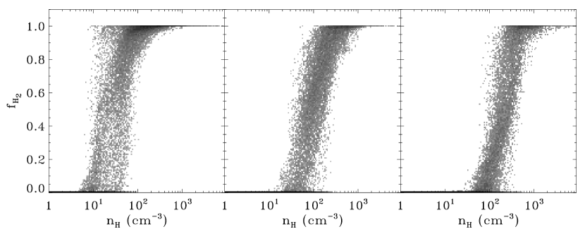
Figure 5.— Molecular hydrogen fraction in level 9 cells, plotted against the total neutral gas number volume density. The grayscale corresponds to the density of binned points on the plane. Left panel: simulation A (solar metallicity); middle panel: simulation B1 (metallicity $0.3$ solar); right panel: simulation B2 (metallicity $0.1$ solar).

Although not apparent in Figure 4, the cold neutral medium undergoes a transition from atomic to fully molecular phase at the gas density of $n_{\rm H}\approx 100\mbox{\,cm}^{-3}$. Figure 5 shows the molecular fraction, $f_{{\rm H}_{2}}=2n_{{\rm H}_{2}}/\left(n_{\rm H\,I}+2n_{{\rm H}_{2}}\right)$, as a function of the total neutral hydrogen volume number density. The three panels correspond to simulations with decreasing metallicity (left panel: simulation A, $Z=Z_{\odot}$; middle panel: simulation B1, $Z=0.3Z_{\odot}$; right panel: simulation B2, $Z=0.1Z_{\odot}$). A sharp transition from fully atomic to fully molecular gas occurs at high gas densities, with the characteristic density of the transition increasing with decreasing metallicity. The gas density at which the molecular fraction is 50% scales with metallicity approximately as

$$n_{\rm t}\simeq 30\left(\frac{Z}{Z_{\odot}}\right)^{-1}\,\,{\rm cm^{-3}}.$$ (7)

This trend is not surprising, as the atomic to molecular transition is facilitated by the dust opacity: when dust opacity is sufficiently high to shield the gas from UV radiation, the transition to molecular medium can occur (self-shielding only becomes dominant at higher molecular fractions). As the metallicity increases, the amount of dust available to shield the gas from UV also increases, and the atomic-to-molecular transition can occur at lower densities.

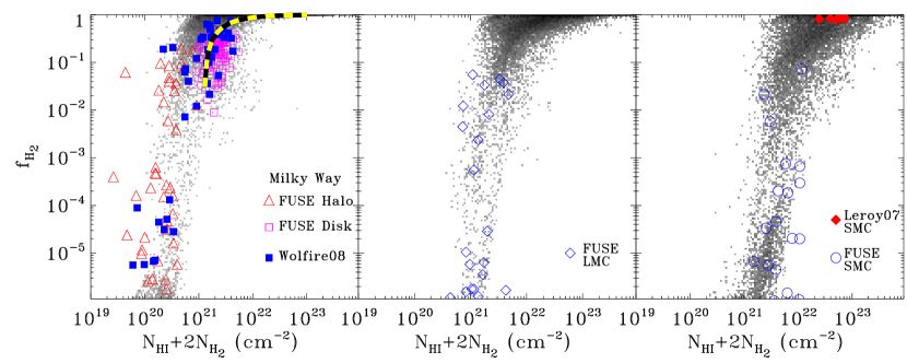
Figure 6.— Molecular hydrogen fraction in level 9 cells, plotted against the total neutral gas column density. The grayscale corresponds to the density of binned points on the plane. Left panel: simulation A (solar metallicity); middle panel: simulation B1 (metallicity $0.3$ solar); right panel: simulation B2 (metallicity $0.1$ solar). Different symbols shows observational data, as follows: open circles: FUSE SMC measurements (compiled by Browning et al. (2003) and Gillmon et al. (2006)); filled diamonds: SMC measurements from Leroy et al. (2007); open diamonds: FUSE LMC measurements; open triangles: FUSE MW Halo measurements; open squares: FUSE MW disk measurements; filled squares: MW measurements from Wolfire et al. (2008). The black/yellow striped line in the left panel shows the location of points with $\Sigma_{\rm H\,I}=10\mbox{\,M${}_{\odot}$/pc${}^{2}$}$.

To compare these results with observational measurements in Figure 6 we plot the molecular fraction against the total neutral hydrogen column density, using a logarithmic vertical scale, for simulations A, B1, B2. We overplot the FUSE measurements of the molecular fraction in the MW halo and disk (left panel), in the LMC (middle panel), and in the SMC (right panel) compiled by Browning et al. (2003) and Gillmon et al. (2006). In the left panel we also plot data for the Milky Way from Wolfire et al. (2008), and on the right panel we show the data for SMC from Leroy et al. (2007). The metallicities of the ISM in these galaxies approximately correspond to the metallicities adopted in the models against which we compare them. In all cases, the column density at which the molecular fractions begin to increase rapidly and the sharpness of the transition are well reproduced in our simulations. For the solar metallicity case, this transition corresponds to the maximum surface density of atomic hydrogen of about $10\mbox{\,M${}_{\odot}$/pc${}^{2}$}$, in concordance with the measurements of molecular and atomic gas surface densities in nearby galaxies (Wong & Blitz, 2002; Blitz & Rosolowsky, 2006; Bigiel et al., 2008). The observed trend of the atomic-to-molecular transition column density to decrease with increasing metallicity is also quantitatively reproduced in our calculations.

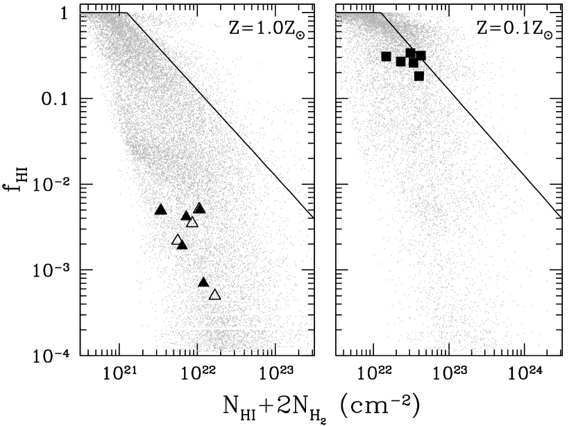
Figure 7.— Atomic hydrogen hydrogen fraction in level 9 cells, plotted against the total gas number density (a complementary figure to Fig. 6). Two panels show solar and 10% solar metallicity cases (we have found no observational data for the LMC case, so we do not show 30% solar metallicity case). Open and filled triangle for the solar metallicity case show measurements from Goldsmith & Li (2005), while filled squares in the 10% solar metallicity panel show Leroy et al. (2007) data. Solid lines in both panels show constraints $\Sigma_{\rm H\,I}=10\mbox{\,M${}_{\odot}$/pc${}^{2}$}$ and $100\mbox{\,M${}_{\odot}$/pc${}^{2}$}$ respectively.

Figure 6 does not illustrate the relationship between the atomic and molecular gas inside mostly molecular gas, when $f_{{\rm H}_{2}}\approx 1$. In order to test our model in that regime, we show in Figure 7 a complement of Figure 6, the atomic hydrogen fraction as a function of the total gas column density. While the measurements of atomic hydrogen fraction in the mostly molecular gas are not numerous (Goldsmith & Li, 2005; Leroy et al., 2007), they provide a useful constraint for our model (see also the Appendix) in the regime where the gas is mostly molecular ($f_{\rm H\,I}\ll 1$).

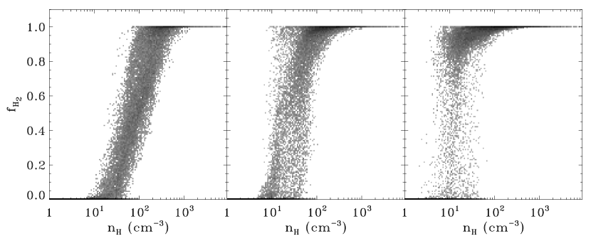
Figure 8.— Molecular hydrogen fraction in level 9 cells, plotted against the total gas number density. Panels from the left to right correspond to clumping factor $C_{\rho}=1$ (simulation C1), $C_{\rho}=10$ (simulation A), and $C_{\rho}=100$ (simulation C2) respectively. The grayscale corresponds to the density of binned points on the plane.

Figure 8 shows the dependence of the transition from atomic to molecular phase on the adopted clumping factor. Although the dependence of the transition on the clumping factor is weaker than on metallicity, it is still appreciable. Increasing the clumping factor steepens the transition and shifts it to lower number densities. Comparison with observations in Figure 6 indicates that the clumping factor of $C_{\rho}=10$ is a good fiducial value. This value is also within the range of clumping factors expected for log-normal PDFs in the theoretical models of molecular clouds (see § 2.2).

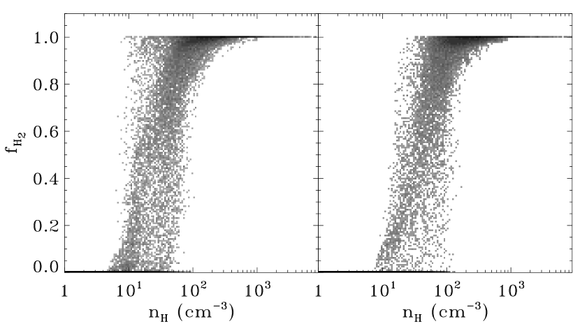
Figure 9.— Molecular hydrogen fraction in level 9 cells, plotted against the volume number density of the total gas. The right panel corresponds to a simulation with 10 times the UV flux (simulation D) of that on the left (simulation A). The grayscale corresponds to the density of binned points on the plane.

Figure 10.— Molecular hydrogen fraction in level 9 cells, plotted against the total gas number density. Left panel: simulation A (star formation recipe SF2); right panel: simulation E (star formation recipe SF1). The grayscale corresponds to the density of binned points on the plane.

In Figure 9 we examine the dependence of the transition from atomic to molecular gas on the UV flux. The right panel (simulation D) represents a UV flux 10 times greater than the one on the left panel (simulation A); that value is at the upper range of observational estimates of the UV field in gamma-ray burst hosts (Chen et al., 2008). Although some differences can be seen, they are much smaller than in the previous figures. The metallicity of the gas, rather than the amount of dissociating radiation, is the primary factor determining the density of atomic to molecular transition. This result may appear counter-intuitive at first, but it is not surprising. Since the UV flux is high, in the optically thin regime the equilibrium fraction of molecular hydrogen is of the order of $10^{-8}$. Thus, gas becomes mostly molecular only when shielding optical depth is of the order of $-\ln(10^{-8})\approx 16$. At this high column density, a factor of 10 increase in the UV flux (and, thus, a factor of 10 decrease in the equilibrium ${{\rm H}_{2}}$ fraction in the optically thin regime) can be fully compensated by the increase of the optical depth (and, thus, the column density) to $-\ln(10^{-9})\approx 18$, which can be achieved, for example, by only $\approx 15\%$ change in the gas density.

This is not to say that the UV flux is not at all important. Recall that the mean flux within our model ISM is already quite high (Figure 2). Without this radiation the abundance of ${{\rm H}_{2}}$ at smaller densities would be quite high (Robertson & Kravtsov, 2008) and transition to fully molecular phase not as steep as indicated by observations (Figure 6). The role of the interstellar UV flux therefore appears to be in controlling the amount of diffuse ${{\rm H}_{2}}$ and maintaining the thermodynamic balance of the cold neutral medium at lower densities, while the transition to the fully molecular phase is controlled primarily by metallicity and clumpiness of the gas.

For completeness, Figure 10 shows dependence of the atomic to molecular phase transition on the adopted star formation recipe. In particular, we compare our fiducial simulation (A) with a star formation timescale which scales with the inverse square root of the gas density (SF2) and simulation E with a constant star formation timescale (SF1). The figure shows that there is no discernible differences between these two recipes (we have also checked that there is no difference when SF3 recipe is adopted). The details of the star formation recipe adopted thus do not affect the transition of atomic to molecular phase, at least within the range of recipes and parameters we considered.

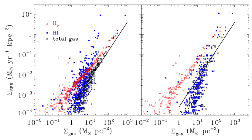
Figure 11.— Sensitivity of the $\Sigma_{\rm SFR}-\Sigma_{\rm gas}$ relation to metallicity. Quantities are averaged over level 3 cells (corresponding, at $z=4$, to a proper scale of $3.2$ kpc). Star formation rates are averaged over 30 Myrs. Each point corresponds to a different level 3 cell in the simulation at $z=4$. Left panel: simulation A (solar metallicity); right panel: simulation B2 (metallicity 0.1 solar). Red triangles: molecular gas; blue squares: atomic gas; black stars: total gas (no He). Solid line: Kennicutt (1998a) law (slope equal to $1.4$, see Eq. 8).

3.2. The Kennicutt-Schmidt relation

In this section we examine the large-scale relation between star formation and gas surface densities (the Kennicutt-Schmidt relation) in the simulated galaxies with the molecular gas model and star formation prescriptions discussed in the previous sections. Figures 11 - 14 show this relation for different choices of the model parameters and star formation prescriptions. Similarly to observational estimates, the star formation rate in this figure was averaged over 30 Myr, the time interval comparable to the characteristic life time of molecular clouds and massive stars. Each point in the figures corresponds to a level 3 cell in the simulation at $z=4$; the physical cell size is 3.3 kpc and thus both the star formation and gas surface densities have been averaged on this scale. In addition to the total gas surface density, the figures also show the dependence of star formation on the surface density of atomic and molecular gas separately. The solid line in each panel corresponds to the best fit to the empirical correlation estimated for nearby massive and starburst galaxies Kennicutt (1998a):

$$\Sigma_{\rm SFR}=2.5\times 10^{-4}\left(\frac{\Sigma_{\rm gas}}{\rm 1\mbox{\,M${}_{\odot}$/pc${}^{2}$}}\right)^{1.4}{\rm\,M_{\odot}\,yr^{-1}kpc^{-2}}\,.$$ (8)

Before we discuss these figures further, it is worth explaining certain features of these plots which may look peculiar to the reader. When one compares the KS relations with different ${{\rm H}_{2}}$ and SF model parameters, $\Sigma_{\rm SFR}$ sometimes does not change, while $\Sigma_{\rm H\,I}$ and $\Sigma_{{\rm H}_{2}}$ change dramatically. This seemingly strange behavior is particularly apparent at high surface densities. The reason is that star formation rate is averaged over $30\mbox{\,Myr}$, while the fraction of ${{\rm H}_{2}}$ and ${\rm H\,I}$ can change on a shorter time scale. Thus, if a region of high surface density becomes fully molecular and forms a population of stars, which then dissociate much of the remaining ${{\rm H}_{2}}$, $\Sigma_{\rm SFR}$ will reflect the fully molecular $\Sigma_{\rm gas}$ and not the current instantaneous $\Sigma_{{\rm H}_{2}}$. The latter reflects the speed with which the molecular gas is able to regenerate after being dissociated by young stars. This speed is controlled by the metallicity and clumpiness of the medium and thus the instantaneous $\Sigma_{{\rm H}_{2}}$ will reflect these dependencies, while $\Sigma_{\rm SFR}$ will not.

Figure 11 shows that the KS relation is quite sensitive to the metallicity of the gas. The left panel corresponds to our fiducial simulation (A) with solar metallicity and the right panel to simulation B2 with metallicity 0.1 solar. While the star formation rate is tightly correlated with the total and ${{\rm H}_{2}}$ surface densities, the correlation with the ${\rm H\,I}$ density exhibits considerable scatter. In addition, the ${\rm H\,I}$ surface density saturates at a relatively low surface density, which depends on metallicity (at $\approx 30\mbox{\,M${}_{\odot}$/pc${}^{2}$}$ for $Z=Z_{\odot}$ and $\approx 100\mbox{\,M${}_{\odot}$/pc${}^{2}$}$ for $Z=0.1Z_{\odot}$). Such saturation is consistent with observations (see, e.g., Kennicutt et al., 2007; Bigiel et al., 2008; Leroy et al., 2008). The surface density at which ${\rm H\,I}$ saturates and its metallicity dependence are of course related to the volume density of the transition from the atomic to molecular phase (see Fig. 6). Given that the latter depends on the choice of the model parameters, the saturation in the KS relation can be used as an additional observational constraint.

The relationship between the star formation rate and the molecular gas surface density (“molecular KS relation”) is less affected by the gas metallicity. Indeed, at a given surface density, the star formation rate is about 3 times higher in a low metallicity gas. This simply reflects the fact that, with our assumptions of a linear relation between the dust-to-gas ratio and gas metallicity, gas at 0.1 solar metallicity forms stars at typical densities that are 10 times higher than in a solar metallicity gas, resulting in about a factor of 3 higher specific star formation rate for our fiducial star formation recipe SF2; respectively, there would be almost no change in the molecular KS relation for the SF1 recipe.

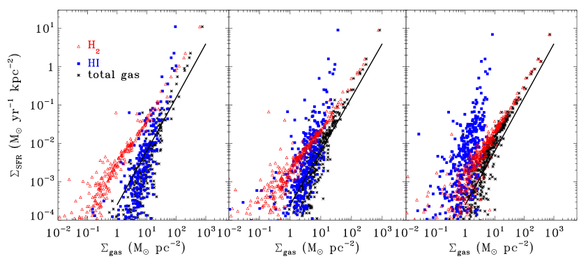
Figure 12.— Sensitivity of the $\Sigma_{\rm SFR}-\Sigma_{\rm gas}$ relation to clumping factor. Points and lines as in Fig. 11. Left panel: $C_{p}=1$ (simulation C1); middle panel: $C_{\rho}=10$ (simulation A); right panel: $C_{p}=100$ (simulation C2).

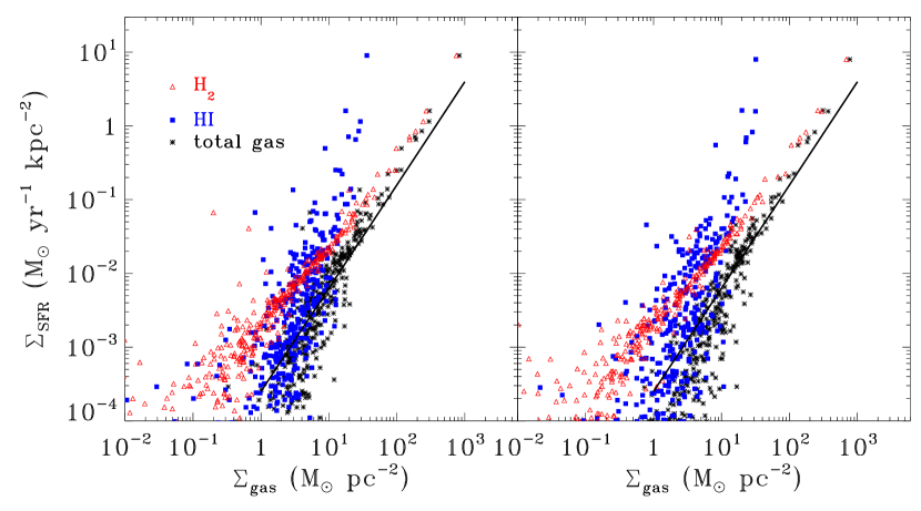
Figure 13.— Sensitivity of the $\Sigma_{\rm SFR}-\Sigma_{\rm gas}$ relation to the UV flux. Points and lines as in Fig. 11. The right panel corresponds to a simulation with 10 times the UV flux (simulation D) than that on the left (simulation A).

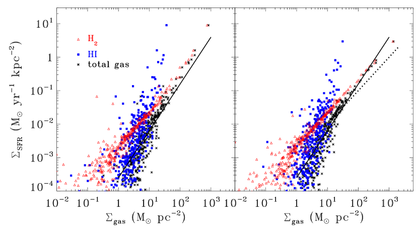
Figure 14.— Sensitivity of the $\Sigma_{\rm SFR}-\Sigma_{\rm gas}$ relation to the star formation recipe. Points and lines as in Fig. 11. Left panel: star formation recipe SF2 (simulation A); right panel: star formation recipe SF1 (simulation E). To illustrate the difference in the slope better, we also show a KS relation with the slope of 1 for $\Sigma>30\mbox{\,M${}_{\odot}$/pc${}^{2}$}$. with a dotted line.

Figure 12 compares the KS relations for the calculations with different clumping factors, $C_{\rho}$. Our fiducial simulation A ($C_{\rho}=10$) is shown in the middle panel, while a simulation with smaller and greater clumping factors (simulation C1 with $C_{\rho}=1$ and simulation C2 with $C_{\rho}=100$) are shown in the left and right panels respectively. Qualitatively, the results are similar to those in Figure 11. However, the figure shows significant sensitivity of the ${\rm H\,I}$ saturation surface density to the clumping factor. Again, this is related to the corresponding dependence of the local volume density of the transition shown in Figure 8. The ${\rm H\,I}$ saturation surface density observed in nearby galaxies can place constraints on the value of the clumping factors. For example, the gas in M51 has metallicity of $Z\approx 2Z_{\odot}$ and its KS relation exhibits saturation at $\Sigma_{\rm H\,I}\approx 30\mbox{\,M${}_{\odot}$/pc${}^{2}$}$. In a larger sample of both massive spirals and dwarf galaxies (with typically $Z<Z_{\odot}$) reported by Leroy et al. (2008), the ${\rm H\,I}$ saturation occurs at $\Sigma_{\rm H\,I}\approx 10-20\mbox{\,M${}_{\odot}$/pc${}^{2}$}$. Comparing these numbers to the KS relations in Figure 12, indicates that the clumping factor required to reproduce these observations (especially at lower than solar metallicities) is quite high, $C_{\rho}\gtrsim 10$. This is, in fact, consistent with observational estimates of the clumping within molecular clouds which indicate that typical ratios of the local to the mean density of a cloud are $\sim 30-100$ (see §3.1.2 in McKee & Ostriker, 2007, and references therein).

As Figure 8 demonstrates, the column density at which the ${\rm H\,I}$ to ${{\rm H}_{2}}$ transition occurs decreases with increasing clumping factor; as a result, the surface density at which ${\rm H\,I}$ saturates decreases with increasing clumping factor. Consequently, the star formation rate scaling with the ${{\rm H}_{2}}$ gas approaches the scaling with the total gas as the clumping factor increases, and become very similar for the highest clumping factor we have used ($C_{\rho}=100$).

The sensitivity of the KS relation to the UV flux is shown in Figure 13. The right panel corresponds to a simulation with 10 times the UV flux (simulation D) than that that of our fiducial run on the left (simulation A). No appreciable changes can be seen between the two panels. The dependence of the global star formation on the UV flux is therefore much weaker than on the metallicity and clumpiness. As we have noted above, this does not mean that the UV flux is not important at all. With the UV flux close to zero the abundance of ${{\rm H}_{2}}$ at smaller densities would be quite high (Robertson & Kravtsov, 2008) and transition to fully molecular phase not as steep as indicated by observations (Figure 6). The role of the interstellar UV flux therefore appears to be in controlling the amount of diffuse ${{\rm H}_{2}}$ and maintaining the thermodynamic balance of the cold neutral medium at lower densities. Beyond certain level, however, the dependence of the results on the UV flux saturates.

Finally, Figure 14 shows the dependence of the scaling on the local star formation recipe used. The left panel corresponds to our fiducial simulation (A), with star formation recipe SF2 (timescale scaling with density), while the right panel corresponds to simulation E with star formation recipe SF1 (constant timescale). The main difference is the slope of the $\Sigma_{\rm SFR}-\Sigma_{{\rm H}_{2}}$ relation. For the constant time scale recipe SF1 the slope is shallower and is close to unity. Note, however, that the slope of the $\Sigma_{\rm SFR}-\Sigma_{\rm gas}$ relation does not change as dramatically and in fact is fairly consistent with the best fit relation of Kennicutt (1998b). This is because this slope is controlled both by the dependence of local star formation efficiency on density and on the dependence of mass fraction of star forming regions on $\Sigma_{\rm gas}$ (Kravtsov, 2003).

4. Discussion and Conclusions

Specifics of star formation modeling in cosmological simulations of galaxy formation have critical impact on the properties of resulting galaxies, such as their star formation histories (and hence luminosity and colors) and morphology. Although significant successes have been achieved using such high-resolution simulations (c.f., Mayer et al., 2008, for a comprehensive review), many challenges remain. In particular, the two likely related challenges are the low efficiency of star formation in low mass systems and the prevalence of thin disks among galaxies. So far, the answer for these challenges was to devise efficient schemes of stellar energy feedback, which is capable of driving outflows (e.g., Springel & Hernquist, 2003; Stinson et al., 2006; Ceverino & Klypin, 2007). However, at least part of the solution may be due to the inherently low efficiency of gas conversion into stars (e.g., Krumholz & McKee, 2005). Indeed, both nearby and high-redshift galaxies provide a variety of clues suggesting that gas conversion into stars in low-mass, low-metallicity galaxies is very inefficient. To explore the effects of such inefficiency on galaxy evolution, a more realistic way of identifying and treating star forming regions is needed. In particular, the global efficiency with which a galaxy converts gas into stars depends on its ability to convert a significant fraction of its gas mass into fully molecular form, within which conditions for star formation can be realized. The latter depends on the small-scale gas properties and local interstellar radiation field. These dependencies are not captured in the standard recipes of star formation.

In this paper we have presented a model for molecular hydrogen formation for cosmological galaxy formation simulations designed to follow the transition from the atomic to molecular phase on the scales of tens of parsecs. The model is applicable in simulations, in which individual star forming regions – the giant molecular complexes – can be identified and their mean internal density estimated reliably, even if internal structure is not resolved. We present a number of tests of the model and illustrate its effects on the global correlation between star formation rate and gas surface density.

The model shows that the transition from atomic to fully molecular phase depends primarily on the metallicity (which we assume is directly related to the dust abundance) and clumpiness of the interstellar medium. The clumpiness simply boosts the formation rate of molecular hydrogen, while dust both serves as a catalyst of ${{\rm H}_{2}}$ formation and as additional shielding from dissociating UV radiation. The upshot is that it is difficult to form fully-shielded giant molecular clouds, while gas metallicity is low. However, once the gas is enriched (say to $Z\sim 0.01-0.1Z_{\odot}$), the subsequent star formation and enrichment can proceed at a much faster rate. This may keep star formation efficiency in the low-mass, low-metallicity progenitors of galaxies very low for a certain period of time. One can think of this as a “feedback” mechanism because it reduces star formation in low metallicity galaxies, but also speeds up star formation once conditions for sustained conversion of a large fraction of gas into fully molecular form are realized.

Molecular fractions in the low-metallicity environments of the nearby dwarf and low surface brightness galaxies are indeed very small (Matthews et al., 2005; Das et al., 2006). Recent observational evidence indicates that the fraction of star forming molecular gas is also small in high-redshift galaxies (e.g., Tumlinson et al., 2007; Wolfe & Chen, 2006). Dependence of the density at which transition from atomic to fully molecular phase occurs on metallicity is indeed observed both in direct measurements for nearby galaxies (see Fig. 6) and in the maximum HI column densities of DLAs of different metallicity at high redshifts (Schaye, 2001) and in the surface density of gas at which surface density of HI saturates in nearby galaxies (Krumholz et al., 2008b).

The UV radiation field is also important in maintaining the cold neutral medium in atomic form (Robertson & Kravtsov, 2008). Our results show, however, that beyond certain flux level the effect of UV radiation on the ability of ISM to form molecular clouds saturates.

We show that the global Kennicutt-Schmidt relation between gas and star formation surface densities is also affected by the local processes controlling conversion of atomic gas into molecular. Our results are qualitatively consistent with those of Robertson & Kravtsov (2008) in that star formation rate dependence on the total gas density can vary depending on the local conditions in the interstellar medium. These results are also consistent with existing detailed studies of the Kennicutt-Schmidt relation in nearby galaxies with lower metallicities and surface densities (e.g., Boissier et al., 2003; Heyer et al., 2004, Wyder et al. 2008, in preparation).

The most recent comprehensive study of the KS relation in the THINGS galaxy sample by Bigiel et al. (2008) shows the KS relation qualitatively similar with our results presented in Figures 11 - 14: $\Sigma_{\rm SFR}$ dependence on $\Sigma_{\rm gas}$ is steep at low gas surface densities, but becomes shallow at larger $\Sigma_{\rm gas}$ values. Interestingly, they find evidence that the slope $n$ of the KS relation at $\Sigma_{\rm gas}\sim 10-100{\rm\,M_{\odot}}$ is $n\approx 1\pm 0.2$, shallower than the canonical value of $n\approx 1.4$. The relation at higher surface densities in star burst galaxies steepens (see Fig. 15 of Bigiel et al., 2008). In the context of our calculations, these results can be interpreted as the systematic change of the internal density of molecular clouds. In our star formation recipes the slope of the large-scale relation depends on the assumed dependence of star formation time scale, $\tau_{\rm sf}$, on the local internal density on the scale of star forming regions, as shown in Figure 14. The steepening of the observed KS relation at high surface densities can thus be interpreted as due to systematic increase of the internal density of molecular clouds at high surface densities, as can be expected in the high-pressure environments of starburst galaxies (e.g. Downes & Solomon, 1998).

Another prediction of our calculations is that the transition at low gas surface densities from a steep to a shallow relation should depend on metallicity. It would thus be interesting to also explore such metallicity dependence in observations. As a first step, one can consider comparison of the KS relation in lower-metallicity dwarf galaxies to the low-$\Sigma_{\rm gas}$ regions in the outskirts of higher-metallicity spirals by Bigiel et al. (2008, see their Fig. 12). Although the KS relation is steep in both of these regimes, the relation for the outskirts of spirals is shifted somewhat to lower $\Sigma_{\rm gas}$, as could be expected from the metallicity dependence.

The above comparisons illustrate that a star formation model of the kind presented in this paper (see also Robertson & Kravtsov, 2008) can be very useful in interpreting the detailed features of the observed KS relation. Conversely, one can use the detailed observations of the KS relation in different regimes (different $\Sigma_{\rm gas}$, different metallicities, etc.) to constrain and tune model parameters. This, in turn, may significantly improve fidelity of star formation modeling in simulations. We plan to present such comparisons as well as applications of our model in fully self-consistent cosmological simulations of galaxy formation in a forthcoming work.

.1. Numerical Considerations

Ideally, in a simulation with infinite spatial resolution, our model should work as designed. In practice, however, the spatial resolution of a simulation is finite. In addition, numerical solutions of partial differential equations always contain truncation errors. In our case, these errors lead to a small, but non-negligible amount of numerical heating and advection that biases the ${{\rm H}_{2}}$ formation model.

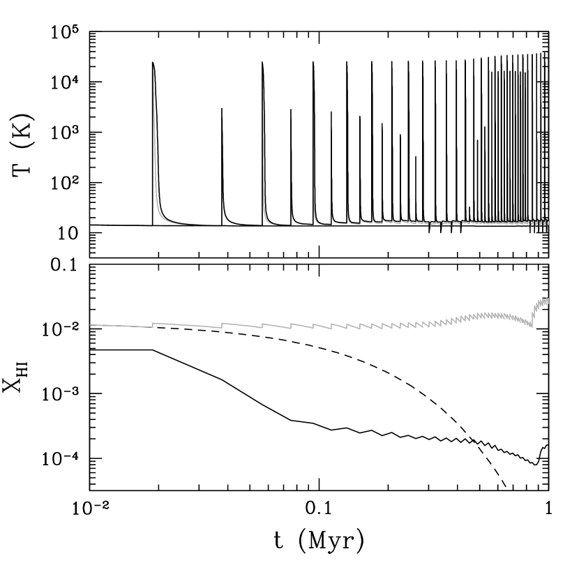
Figure 15.— Evolution of the gas temperature (top) and ${\rm H\,I}$ fraction (bottom) for a single, fully molecular cell in our fiducial run. The black dashed line shows a test calculation when the cell is evolved in isolation at constant gas density and constant radiation field (without any hydrodynamic effects). The light gray solid line is the evolution of the same cell in a full cosmological simulation - notice the numerical heating and advection, appearing as jumps in temperature and neutral hydrogen fraction at regular intervals corresponding to individual hydrodynamic time steps. The solid black line is for the same test with the numerical correction (3).

An example of such diffusion is shown in Figure 15, where we compare an ideal, single zone (i.e. without any hydrodynamic effects) evolution of a typical cell inside molecular clouds (i.e. with molecular fraction above 99% - shown as black dashed lines) with the evolution of this cell in a real cosmological simulation. Because our resolution is finite, gas motions across individual cells are not fully resolved; in a Riemann code the truncation errors from such incomplete resolution lead to cells being heated at each time step. This numerical heating is not too serious, since the gas cooling time is very short; however, a more serious artifact is the numerical advection of atomic gas inside molecular clouds. The gray line on the bottom panel shows the evolution of the atomic hydrogen fraction in that cell - at each hydrodynamic time step there is a small (about 10%) increase in the atomic hydrogen fraction. This amount is not large, but it happens at every time step, and so, effectively, there is a numerical flux of atomic hydrogen into molecular clouds, with the corresponding opposite flux of molecular hydrogen out of molecular gas.

We emphasize that this is a numerical artifact: the transition between molecular and atomic phases is so sharp that few numerical schemes are able to treat it perfectly. As a numerical artifact, this effect is actually rather small - 10% jump in $f_{\rm H\,I}\sim 0.01$ corresponds to the relative numerical diffusion of only about $10^{-3}$ per time step. This effect is only important because the atomic hydrogen fraction inside molecular clouds is of the same order, about $10^{-3}$, or even less.

In order to mitigate this numerical advection, we adopt the following, entirely empirical approach. The numerical advection can be thought of as an additive increase in the atomic hydrogen fraction per time step,

$$X_{{\rm H\,I}}^{\rm Num}=X_{{\rm H\,I}}^{\rm True}+\Delta X_{{\rm H\,I}}.$$

If we multiply the “numerical” value $X_{{\rm H\,I}}^{\rm Num}$ at the end of each hydrodynamic time step by the correction factor

$$f_{\rm Num}=\left(1+\frac{\Delta X_{{\rm H\,I}}}{X_{{\rm H\,I}}^{\rm True}}\right)^{-1},$$

then we would remove the numerical advection completely. Unfortunately, we do not have any way to measure both $X_{{\rm H\,I}}^{\rm True}$ and $\Delta X_{{\rm H\,I}}$ in a self-consistent way (for example, keeping track of $X_{{\rm H\,I}}$ without hydrodynamic advection would violate Galilean invariance). Because the numerical advection per time step is not large, we can use $X_{{\rm H\,I}}^{\rm Num}$ (the value we get in the simulation) instead of $X_{{\rm H\,I}}^{\rm True}$ in the expression for $f_{\rm Num}$, but the factor $\Delta X_{{\rm H\,I}}$ needs to be deduced heuristically.

We choose to define $\Delta X_{{\rm H\,I}}$ as

$$\Delta X_{{\rm H\,I}}\equiv\alpha\sigma_{\rm cell}\frac{\Delta t}{\Delta x}X_{\rm H},$$ (1)

where $\alpha$ is a numerical coefficient of the order of unity, $\sigma_{\rm cell}$ is the gas velocity dispersion at the cell scale, computed in each cell $(i,j,k)$ from its six neighbors,

$$\sigma_{\rm cell}^{2}(i,j,k)\equiv\frac{1}{6}\left[\left(\vec{v}_{i+1,j,k}-\vec{v}_{i,j,k}\right)^{2}+\left(\vec{v}_{i-1,j,k}-\vec{v}_{i,j,k}\right)^{2}+\left(\vec{v}_{i,j+1,k}-\vec{v}_{i,j,k}\right)^{2}+...\right],$$ (2)

and $\Delta t$ and $\Delta x$ are the numerical time step and the cell size (which is, in fact, different for different cells on an adaptively refined mesh in our simulations). The factor $X_{\rm H}$ encapsulates our assumption that the gas is mostly atomic and neutral just outside molecular clouds.

Equation (1) has the correct properties for an expression describing numerical advection. First, it vanishes in the limit of $\Delta t\rightarrow 0$. We have actually verified, by running test simulations with reduced time steps, that the numerical advection effect shown in Figure 15 scales linearly with the time step $\Delta t$. Second, equation 1 is Galilean invariant and depends on the local variation in the gas velocity, i.e. on the quantity that determines hydrodynamic advection (beyond trivial uniform translation). Third, $\Delta X_{{\rm H\,I}}$ does not actually diverge in the limit $\Delta x\rightarrow 0$, because for a fully resolved flow

$$\sigma_{\rm cell}=\frac{1}{3}\left(\sum_{i,j}\frac{\partial v^{i}}{\partial x^{j}}\frac{\partial v^{i}}{\partial x^{j}}\right)^{1/2}\Delta x.$$

Thus, our heuristic numerical advection correction factor becomes

$$f_{\rm Num}\approx\left(1+\alpha\sigma_{\rm cell}\frac{\Delta t}{\Delta x}\frac{X_{\rm H}}{X_{{\rm H\,I}}}\right)^{-1}.$$ (3)

This form for the numerical correction is also rather insensitive to the specific choice of the coefficient $\alpha$: varying $\alpha$ from 0.5 to 2 changes atomic hydrogen fractions inside molecular clouds and star formation rates by less than their natural scatter.

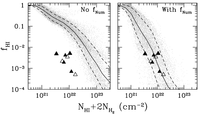
Figure 16.— Atomic hydrogen fraction as a function of the total neutral hydrogen column density for two test runs: a run without numerical correction (3; left) and a run with numerical correction included (right). Gray points show individual simulation cells, while the black solid and dashed line show the mean and $\pm 1\sigma$. Black and open triangles are observational measurements from Goldsmith & Li (2005).

The correction factor (3), being heuristic, does not completely correct for numerical advection on a cell-by-cell basis; it is valid only in a statistical sense. As Figure 15 shows, evolution of the abundance in a test cell with the correction factor included does not match a single zone calculation (although, a single zone calculation excludes not only unphysical numerical advection, but physical real advection as well, and should not be taken as a correct solution). The only justification for the factor (3) is Figure 16, which shows a comparison of the atomic hydrogen fractions that we find in our simulations with the observational points from Goldsmith & Li (2005). Without the correction (3) the observational points cannot be reproduced, while with the correction we get a good match to the observational constraints.

References

- Abel et al. (1997) Abel, T., Anninos, P., Zhang, Y., & Norman, M. L. 1997, New Astronomy, 2, 181
- Bigiel et al. (2008) Bigiel, F., Leroy, A., Walter, F., de Block, W., Brinks, E., Madore, B., & Thornley, M. 2008, AJ in press
- Blitz et al. (2007) Blitz, L., Fukui, Y., Kawamura, A., Leroy, A., Mizuno, N., & Rosolowsky, E. 2007, in Protostars and Planets V, ed. B. Reipurth, D. Jewitt, & K. Keil, 81–96
- Blitz & Rosolowsky (2006) Blitz, L. & Rosolowsky, E. 2006, ApJ submitted (astro-ph/0605035)
- Blitz & Shu (1980) Blitz, L. & Shu, F. H. 1980, ApJ, 238, 148
- Boissier et al. (2003) Boissier, S., Prantzos, N., Boselli, A., & Gavazzi, G. 2003, MNRAS, 346, 1215
- Booth et al. (2007) Booth, C. M., Theuns, T., & Okamoto, T. 2007, MNRAS, 376, 1588
- Brooks et al. (2007) Brooks, A. M., Governato, F., Booth, C. M., Willman, B., Gardner, J. P., Wadsley, J., Stinson, G., & Quinn, T. 2007, ApJ, 655, L17
- Browning et al. (2003) Browning, M. K., Tumlinson, J., & Shull, J. M. 2003, ApJ, 582, 810
- Burke & Hollenbach (1983) Burke, J. R. & Hollenbach, D. J. 1983, ApJ, 265, 223
- Cazaux & Spaans (2004) Cazaux, S. & Spaans, M. 2004, ApJ, 611, 40
- Ceverino & Klypin (2007) Ceverino, D. & Klypin, A. 2007, ArXiv e-prints, 712
- Chen et al. (2008) Chen, H.-W., Perley, D. A., Pollack, L. K., Prochaska, J. X., Bloom, J. S., Dessauges-Zavadsky, M., Pettini, M., Lopez, S., Dall’Aglio, A., & Becker, G. D. 2008, ArXiv e-prints
- Croft et al. (2008) Croft, R. A. C., Di Matteo, T., Springel, V., & Hernquist, L. 2008, ArXiv e-prints, 803
- Das et al. (2006) Das, M., O’Neil, K., Vogel, S. N., & McGaugh, S. 2006, ApJ, 651, 853
- Downes & Solomon (1998) Downes, D. & Solomon, P. M. 1998, ApJ, 507, 615
- Draine (1978) Draine, B. T. 1978, ApJS, 36, 595
- Draine & Bertoldi (1996) Draine, B. T. & Bertoldi, F. 1996, ApJ, 468, 269
- Elmegreen (1989) Elmegreen, B. G. 1989, ApJ, 338, 178
- Elmegreen (1993) —. 1993, ApJ, 411, 170
- Galli & Palla (1998) Galli, D. & Palla, F. 1998, A&A, 335, 403
- Gibson et al. (2008) Gibson, B. K., Courty, S., Sanchez-Blazquez, P., Teyssier, R., House, E. L., Brook, C. B., & Kawata, D. 2008, ArXiv e-prints, 808
- Gillmon et al. (2006) Gillmon, K., Shull, J. M., Tumlinson, J., & Danforth, C. 2006, ApJ, 636, 891
- Glover & Abel (2008) Glover, S. C. O. & Abel, T. 2008, ArXiv e-prints, 803
- Glover & Jappsen (2007) Glover, S. C. O. & Jappsen, A.-K. 2007, ApJ, 666, 1
- Glover & Mac Low (2007) Glover, S. C. O. & Mac Low, M.-M. 2007, ApJS, 169, 239
- Gnedin & Abel (2001) Gnedin, N. Y. & Abel, T. 2001, New Astronomy, 6, 437
- Goldsmith & Li (2005) Goldsmith, P. F. & Li, D. 2005, ApJ, 622, 938
- Governato et al. (2007) Governato, F., Willman, B., Mayer, L., Brooks, A., Stinson, G., Valenzuela, O., Wadsley, J., & Quinn, T. 2007, MNRAS, 374, 1479
- Heyer et al. (2004) Heyer, M. H., Corbelli, E., Schneider, S. E., & Young, J. S. 2004, ApJ, 602, 723
- Hollenbach & McKee (1979) Hollenbach, D. & McKee, C. F. 1979, ApJS, 41, 555
- Kennicutt (1989) Kennicutt, R. C. 1989, ApJ, 344, 685
- Kennicutt (1998a) —. 1998a, ApJ, 498, 541
- Kennicutt (1998b) Kennicutt, Jr., R. C. 1998b, ApJ, 498, 541
- Kennicutt et al. (2007) Kennicutt, Jr., R. C., Calzetti, D., Walter, F., Helou, G., Hollenbach, D. J., Armus, L., Bendo, G., Dale, D. A., Draine, B. T., Engelbracht, C. W., Gordon, K. D., Prescott, M. K. M., Regan, M. W., Thornley, M. D., Bot, C., Brinks, E., de Blok, E., de Mello, D., Meyer, M., Moustakas, J., Murphy, E. J., Sheth, K., & Smith, J. D. T. 2007, ApJ, 671, 333
- Kravtsov (1999) Kravtsov, A. V. 1999, Ph.D. Thesis
- Kravtsov (2003) —. 2003, ApJ, 590, L1
- Kravtsov et al. (2002) Kravtsov, A. V., Klypin, A., & Hoffman, Y. 2002, ApJ, 571, 563
- Kravtsov et al. (1997) Kravtsov, A. V., Klypin, A. A., & Khokhlov, A. M. 1997, ApJS, 111, 73
- Krumholz & McKee (2005) Krumholz, M. R. & McKee, C. F. 2005, ApJ, 630, 250
- Krumholz et al. (2008a) Krumholz, M. R., McKee, C. F., & Tumlinson, J. 2008a, ArXiv e-prints, 805
- Krumholz et al. (2008b) —. 2008b, ApJ in press (astro-ph/0805.2947)
- Krumholz & Tan (2007a) Krumholz, M. R. & Tan, J. C. 2007a, ApJ, 654, 304
- Krumholz & Tan (2007b) —. 2007b, ApJ, 654, 304
- Leroy et al. (2008) Leroy, A., Bigiel, F., Walter, F., Brinks, E., de Blok, W. J. G., & Madore, B. 2008, in Astronomical Society of the Pacific Conference Series, Vol. 387, Astronomical Society of the Pacific Conference Series, ed. H. Beuther, H. Linz, & T. Henning, 408–+
- Leroy et al. (2007) Leroy, A., Bolatto, A., Stanimirovic, S., Mizuno, N., Israel, F., & Bot, C. 2007, ApJ, 658, 1027
- Matthews et al. (2005) Matthews, L. D., Gao, Y., Uson, J. M., & Combes, F. 2005, AJ, 129, 1849
- Mayer et al. (2008) Mayer, L., Governato, F., & Kaufmann, T. 2008, ArXiv e-prints, 801
- McKee & Ostriker (2007) McKee, C. F. & Ostriker, E. C. 2007, ARA&A, 45, 565
- Oppenheimer & Davé (2008) Oppenheimer, B. D. & Davé, R. 2008, MNRAS, 387, 577
- Ostriker et al. (2001) Ostriker, E. C., Stone, J. M., & Gammie, C. F. 2001, ApJ, 546, 980
- Padoan et al. (1997) Padoan, P., Jones, B. J. T., & Nordlund, A. P. 1997, ApJ, 474, 730
- Pelupessy et al. (2006) Pelupessy, F. I., Papadopoulos, P. P., & van der Werf, P. 2006, ApJ, 645, 1024
- Razoumov (2008) Razoumov, A. O. 2008, ArXiv e-prints, 808
- Robertson & Kravtsov (2008) Robertson, B. E. & Kravtsov, A. V. 2008, ApJ, 680, 1083
- Scannapieco et al. (2008) Scannapieco, C., Tissera, P. B., White, S. D. M., & Springel, V. 2008, MNRAS, 957
- Schaye (2001) Schaye, J. 2001, ApJ, 562, L95
- Schmidt (1959) Schmidt, M. 1959, ApJ, 129, 243
- Schmidt (1963) —. 1963, ApJ, 137, 758
- Shapiro & Kang (1987) Shapiro, P. R. & Kang, H. 1987, ApJ, 318, 32
- Springel & Hernquist (2003) Springel, V. & Hernquist, L. 2003, MNRAS, 339, 289
- Stinson et al. (2006) Stinson, G., Seth, A., Katz, N., Wadsley, J., Governato, F., & Quinn, T. 2006, MNRAS, 373, 1074
- Tasker & Bryan (2008) Tasker, E. J. & Bryan, G. L. 2008, ApJ, 673, 810
- Tassis et al. (2008) Tassis, K., Kravtsov, A. V., & Gnedin, N. Y. 2008, ApJ, 672, 888
- Tumlinson et al. (2007) Tumlinson, J., Prochaska, J. X., Chen, H.-W., Dessauges-Zavadsky, M., & Bloom, J. S. 2007, ApJ, 668, 667
- Wolfe & Chen (2006) Wolfe, A. M. & Chen, H.-W. 2006, ApJ, 652, 981
- Wolfire et al. (2003) Wolfire, M. G., McKee, C. F., Hollenbach, D., & Tielens, A. G. G. M. 2003, ApJ, 587, 278
- Wolfire et al. (2008) Wolfire, M. G., Tielens, A. G. G. M., Hollenbach, D., & Kaufman, M. J. 2008, ArXiv e-prints, 803
- Wong & Blitz (2002) Wong, T. & Blitz, L. 2002, ApJ, 569, 157