Introduction

Elongated particles form liquid crystalline structures at high densities. For example, they often exhibit a nematic phase, where the particles align along one preferred direction (the director), while their positions are disordered, like in a fluid. For symmetry reasons, the phase transition between the nematic phase (N) and the fully disordered isotropic phase (I) must be first order[1]. Hence the two phases coexist in a certain parameter regime, and are separated by a nematic-isotropic (NI)-interface. The properties of that interface are intriguing for several reasons: Since it separates two fluid phases, the interfacial tension of a planar interface of given orientation $\mathbf{N}$ should be isotropic – the free energy cost of increasing the interfacial area should not depend on the direction in which the area has been extended. On the other hand, the interface interacts with the adjacent, anisotropic, nematic fluid – for example, it orients the director (“surface anchoring”) – and one would expect this to have an influence on the interface. Hence, it should also exhibit anisotropic features.

The role of the interfacial tension for the interfacial structure can be assessed by studying the fluctuations of the interface positions, the “capillary waves”. For interfaces between two simple fluids, the theory of capillary waves is quite simple: Let us consider a planar interface oriented in the $z$-direction with the projected area $A$, neglect overhangs, and parametrize the local interface position by a single-valued function $h(x,y)$. Fluctuations enlarge the interfacial area and thus cost the free energy[2, 3, 4]

$${\cal F}\{h\}=\gamma\int\!\!\mbox{d}x\>\mbox{d}y\>\sqrt{1+(\partial_{x}h)^{2}+(\partial_{y}h)^{2}}\approx\gamma A+\frac{\gamma}{2}\int\!\!\mbox{d}x\>\mbox{d}y\>\big{[}(\partial_{x}h)^{2}+(\partial_{y}h)^{2}\big{]}$$ (1)

with the interfacial tension $\gamma$. Based on this functional, the thermal height fluctuations $\langle|h(\mbox{$\mathbf{q}$})|^{2}\rangle$ at given wave vector $\mathbf{q}$ can be calculated in a straightforward manner. One obtains the capillary wave spectrum

$$\langle|h(\mbox{$\mathbf{q}$})|^{2}\rangle=\mbox{${k_{{}_{B}}}$}T/\gamma q^{2}.$$ (2)

At a NI interface, the situation is more complicated. The capillary wave fluctuations are then determined by at least three factors, namely, (i) the interfacial tension, (ii) the surface anchoring, and (iii) the elasticity of the nematic bulk, i.e., the elastic response of the nematic fluid to local director variations.

In the present paper, we shall review recent work that has shed light on the interplay of these three factors. The paper is organized as follows. In the next section, we discuss large-scale simulations of NI interfaces in model liquid crystals, which have allowed to study in detail the capillary wave spectrum in these systems. In section three, a Landau-de Gennes theory of capillary waves is presented. The predictions of this theory are compared with the simulations in section four. Finally, we summarize and conclude with a brief outlook on nonequilibrium interfaces.

Computer Simulations

Computer simulations of equilibrium NI interfaces were carried out for two standard model liquid crystals: Systems of ellipsoids[5, 6] and systems of spherocylinders[7, 8, 9]. In two of these studies[6, 9], the system sizes were large enough that capillary waves could be investigated in detail. These shall be compared with each other.

The model ellipsoids interact with each other via a soft, repulsive, Weeks-Chandler-Andersen-type[10] potential

$$V(\mbox{$\mathbf{u}$}_{i},\mbox{$\mathbf{u}$}_{j},\mbox{$\mathbf{r}$}_{ij})=\left\{\begin{array}[]{ll}4\epsilon(X^{-12}-X^{-6}+\frac{1}{4})&\mbox{ $X^{6}>\frac{1}{2}$}\\ 0&\mbox{ otherwise}\end{array}\right.$$ (3)

with

$$X=\frac{r-\sigma(\mbox{$\mathbf{u}$}_{i},\mbox{$\mathbf{u}$}_{j},\hat{\mbox{$\mathbf{r}$}}_{ij})+\sigma_{s}}{\sigma_{s}},$$ (4)

where $\sigma_{s}$ is the diameter of the ellipsoids, $\mbox{$\mathbf{u}$}_{i}$ and $\mbox{$\mathbf{u}$}_{j}$ are the orientations of ellipsoids $i$ and $j$, $\hat{\mbox{$\mathbf{r}$}}_{ij}$ is the unit vector connecting the centers of the two ellipsoids, and the shape function[11]

$$\sigma({\bf u}_{i},{\bf u}_{j},{\hat{\bf r}})=\sigma_{s}\Big{\{}1-\frac{\chi}{2}\Big{[}\frac{({\bf u}_{i}\cdot{\hat{\bf r}}+{\bf u}_{j}\cdot{\hat{\bf r}})^{2}}{1+\chi{\bf u}_{i}\cdot{\bf u}_{j}}+\frac{({\bf u}_{i}\cdot{\hat{\bf r}}-{\bf u}_{j}\cdot{\hat{\bf r}})^{2}}{1-\chi{\bf u}_{i}\cdot{\bf u}_{j}}\Big{]}\Big{\}}^{-1/2}$$ (5)

approximates the contact distance between hard ellipsoids of elongation $\kappa$ with $\chi=(\kappa^{2}-1)/(\kappa^{2}+1)$. The temperature was chosen $\mbox{${k_{{}_{B}}}$}T=\epsilon$.

The spherocylinders are taken to be hard rods with semi-spherical caps, i.e., lines of length $L$, which may not come closer to each other than a distance $D$ (the diameter of the rods).

The elongation of the particles, $\kappa$ or $L/D$, respectively, was chosen 15 in both cases. The simulations were carried out in the $NVT$-ensemble with roughly $N\approx 100.000$ particles in an elongated simulation box with side length ratios $L_{x}:L_{y}:L_{z}\equiv 1:1:2$ and periodic boundary conditions. The simulation method was Molecular dynamics in the case of the ellipsoids[6], and Monte Carlo in the case of the hard rods[9]. By choosing a mean density between the densities of the nematic and isotropic phase at coexistence, phase separation into a nematic and an isotropic slab was enforced. The equilibrated systems thus contained two planar NI interfaces with orientation normals $\mathbf{N}$ parallel to the long axis of the simulation box. Both for ellipsoids and hard rods, the director in the nematic phase spontaneously aligned in the direction parallel to the interface (planar anchoring). Normal anchoring could be studied as well, but had to be enforced, e.g., by choosing special boundary conditions[5], or by preparing an initial configuration that contains a nematic slab with normal orientation[9]. Here, we will almost exclusively discuss planar anchoring. To analyze the capillary wave spectrum, the simulation box was split into columns (blocks) $B\times B\times L_{z}$, and the local interface positions were determined separately in each block. This gave two interface topographies $h(x,y)$ for every configuration, which could then be Fourier transformed to obtain the capillary wave spectrum, $|h(\mbox{$\mathbf{q}$})|^{2}$ (cf. Appendix). More details on the simulation and the data analysis can be found in Refs. 6 and 9.

Table 1 summarizes the main properties of our model systems at coexistence. Most of the data are compiled from earlier publications[5, 6, 8, 9], but the table also shows new, previously unpublished results. In particular, it gives the Frank elastic constants[1, 12] $K_{1},K_{2},K_{3}$ of the ellipsoid system in the nematic phase, which we have evaluated in order to use them for a quantitative comparison between theory and simulation (see below). To this end, separate simulations of a homogeneous system at the density of the nematic phase were conducted, and the order tensor fluctuations were analyzed, following a procedure described in Refs. 13 and 14.

Table 1: Properties of our model systems at NI coexistence. Numbers in brackets indicate errors in the last digit.

	Ellipsoids	Hard rods
densities	$\rho_{N}=0.0181(1)/\sigma_{s}^{3}$	$\rho_{N}=0.027/D^{3}$
	$\rho_{I}=0.0149(1)/\sigma_{s}^{3}$	$\rho_{I}=0.023/D^{3}$
reduced densities	$\rho_{N}^{*}=0.192$	$\rho_{N}^{*}=0.22$
	$\rho_{I}^{*}=0.158$	$\rho_{I}^{*}=0.193$
$\rho^{*}=\rho/\rho_{cp}$	$\rho_{cp}=\sqrt{2}/15$	$\rho_{cp}=2/(\sqrt{2}+15\sqrt{3})$
order parameter	$S_{N}=0.74$[5]	$S_{N}\approx 0.7$
Frank	$K_{1}=0.78(2)$
elastic constants	$K_{2}=0.32(2)$ at $\rho=0.018$
(nematic phase)	$K_{3}=3.61(5)$
interfacial tension	from pressure tensor[5, 6]	from histogram method[8]
planar anchoring†	$\gamma_{IN}=0.011(4)\mbox{${k_{{}_{B}}}$}T/\sigma_{s}^{2}$[5]	$\gamma_{IN}=0.0064\mbox{${k_{{}_{B}}}$}T/D^{2}$[8]
	$\gamma_{IN}=0.009(3)\mbox{${k_{{}_{B}}}$}T/\sigma_{s}^{2}$[6]
normal anchoring	$\gamma_{IN}=0.015(4)\mbox{${k_{{}_{B}}}$}T/\sigma_{s}^{2}$[5]
interfacial width‡	$w\approx 7.3\sigma_{s}$	$w\approx 10.6D$

^† The two values for the ellipsoids were obtained in simulations with different system sizes. They agree within the error.
^‡ The interfacial width has been determined by a fit of the local order parameter profile to a $\tanh$ profile, $\tanh((z-z_{0})/w$. Due to the effect of capillary waves, it depends on the lateral system size. The values given here correspond to local profiles evaluated in blocks of lateral size $B=2\kappa\sigma_{s}$ (ellipsoids)[6] and $B=2L$ (rods)[9].

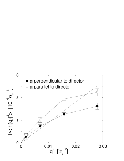
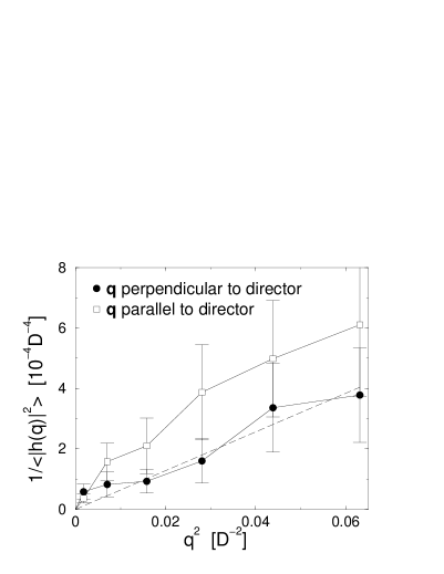
Figure 1: Inverse mean-squared Fourier components of the interface position $h$ vs. wave vector $\mathbf{q}$ squared for $\mathbf{q}$ parallel and perpendicular to the director $\mbox{$\mathbf{n}$}_{0}$. Left: Ellipsoids (similar to Ref. 6; data taken from Ref. 15). Right: Hard rods (similar to Ref. 9, different data set). The straight dashed lines indicate the prediction of Eq. (2) with the interfacial tension taken from Table 1, $\gamma=0.009\mbox{${k_{{}_{B}}}$}T/\sigma_{s}^{2}$ (ellipsoids) and $\gamma=0.0064\mbox{${k_{{}_{B}}}$}T/D^{2}$ (hard rods). Remarkably, it seems to fit the lower branch ($\mbox{$\mathbf{q}$}\perp\mbox{$\mathbf{n}$}_{0}$) rather well in both systems.

The capillary wave spectra for the two model systems are shown in Fig. 1. The capillary waves are clearly anisotropic: In the direction of the director, they are suppressed by a factor 0.3-0.5, compared to those in the perpendicular direction. Nevertheless, they still roughly follow the proportionality law $1/\langle|h(\mbox{$\mathbf{q}$})|^{2}\rangle\sim q^{2}$ predicted by Eq. (2). Deviations are observed in the ellipsoid system for wavelengths comparable to the particle length, $2\pi/q\sim 3\kappa\sigma_{s}$. In the hard rod system, the proportionality persists over the whole accessible wave vector range. Hence it seems that Eq. (2) would provide a reasonable description of our data, provided the interfacial tension $\gamma$ were allowed to depend on the direction of the wave vector, $\mathbf{q}$. On the other hand, we have pointed out in the introduction that the macroscopic surface tension between two fluid phases must be isotropic. To resolve this apparent contradiction, a Landau-de Gennes type theory of capillary wave fluctuations at NI interfaces has been developed[16]. It shall be presented next.

Theory

The Landau-de Gennes theory is based on a free energy expansion in powers of a symmetric and traceless (3$\times$3) order tensor field ${\bf Q}(\mbox{$\mathbf{r}$})$[1]

$$F=\int\!\!\!d^{3}\!\!r\,\Big{\{}\frac{A}{2}\mbox{Tr}(\mbox{${\bf Q}$}^{2})\!+\!\frac{B}{3}\mbox{Tr}(\mbox{${\bf Q}$}^{3})\!+\!\frac{C}{4}\mbox{Tr}(\mbox{${\bf Q}$}^{2})^{2}+\>\frac{L_{1}}{2}\partial_{i}Q_{jk}\partial_{i}Q_{jk}+\frac{L_{2}}{2}\partial_{i}Q_{ij}\partial_{k}Q_{kj}\Big{\}},$$ (6)

with $B<0$ close to the NI transition. If biaxiality can be neglected (both in our ellipsoid and hard rod system, the maximum value of the biaxiality near the NI interface was less than 0.06), the order tensor can be written as[17] $Q_{ij}(\mbox{$\mathbf{r}$})=\frac{1}{2}S(\mbox{$\mathbf{r}$})(3n_{i}(\mbox{$\mathbf{r}$})n_{j}(\mbox{$\mathbf{r}$})-\delta_{ij})$, where $S(\mbox{$\mathbf{r}$})$ is the local scalar order parameter, and $\mathbf{n}$ a unit vector characterizing the local director. For further simplification, we introduce “natural” units $S_{0}=-{2B}/{9C}$, $\xi_{0}=2\sqrt{{(L_{1}+L_{2}/6)}/{3C}}\>{S_{0}^{-1}}$, and $\epsilon_{0}=({3C}/{16})S_{0}^{4}\xi_{0}^{3}$ for the order parameter, the length, and the energy, and rescale all quantities by these units. The free energy functional (6) then takes the form[18]

$$F=3\int d^{3}r\>\{f+g_{1}+g_{2}\}\quad\mbox{with}\quad f=S^{2}((S-1)^{2}+t),$$ (7)

$$g_{1} = (\nabla\cdot S)^{2}+\alpha(\mbox{$\mathbf{n}$}\cdot\nabla S)^{2}+4\alpha S\Big{(}(\nabla\cdot\mbox{$\mathbf{n}$})(\mbox{$\mathbf{n}$}\cdot\nabla S)+\frac{1}{2}(\mbox{$\mathbf{n}$}\times\nabla\times\mbox{$\mathbf{n}$})(\nabla S)\Big{)},$$

$$g_{2} = S^{2}\Big{(}(3+2\alpha)(\nabla\mbox{$\mathbf{n}$})^{2}+(3-\alpha)(\mbox{$\mathbf{n}$}\cdot\nabla\times\mbox{$\mathbf{n}$})^{2}+\>(3+2\alpha)(\mbox{$\mathbf{n}$}\times\nabla\times\mbox{$\mathbf{n}$})^{2}\Big{)}.$$

with the two dimensionless parameters,

$$t=\frac{1}{4}A\frac{S_{0}^{2}\xi_{0}^{3}}{\epsilon_{0}}-1,\qquad\mbox{and}\qquad\alpha=\frac{1}{2}\>\frac{L_{2}}{(L_{1}+L_{2}/6)}.$$ (8)

The parameter $t$ gives the distance from NI coexistence and becomes zero at coexistence. The parameter $\alpha$ characterizes the response of the system to order parameter and director variations. In Eq. (7), the first term, $f(S)$, is the free energy density of a homogeneous system, the second term, $g_{1}$, accounts for the effect of order parameter variations, and the last term, $g_{2}$, corresponds to the Frank elastic energy of a nematic fluid with spatially varying director. This last term relates the free energy functional (7) to the well-known Frank elastic energy[1, 12]

$$F_{F}=\frac{1}{2}\int\!d^{3}\!r\,\Big{\{}K_{1}(\nabla\mbox{$\mathbf{n}$})^{2}+K_{2}(\mbox{$\mathbf{n}$}\cdot\nabla\times\mbox{$\mathbf{n}$})^{2}+K_{3}(\mbox{$\mathbf{n}$}\times\nabla\times\mbox{$\mathbf{n}$})^{2}\Big{\}}$$ (9)

and allows to identify the three Frank elastic constants splay ($K_{1}$), twist ($K_{2}$), and bend ($K_{3}$). We note that Eq. (7) predicts $K_{1}=K_{3}$, whereas experimentally and in simulations (see Table 1), the parameter $K_{3}$ is usually much higher than $K_{1}$. To improve the theory in this respect, one would have to include higher powers of ${\bf Q}$ in the expansion (6).

Minimizing the free energy (7) with the boundary conditions $S=0$ at $z\to-\infty$, $S=1$ at $z\to\infty$ and fixed director $\mbox{$\mathbf{n}$}\equiv\mbox{$\mathbf{n}$}_{0}$ yields the mean-field structure of a planar NI interface at fixed anchoring angle $\cos\theta=\mbox{$\mathbf{n}$}_{0,z}\equiv(\mbox{$\mathbf{n}$}_{0}\mbox{$\mathbf{N}$})$ ($\mathbf{N}$ being the interface normal): The order parameter adopts a tanh profile, $S(z)=S_{0}\bar{S}(z/w)$ with

$$\bar{S}(\tau)=\frac{1}{2}(1+\tanh(\tau))\qquad\mbox{and the width}\qquad w=2\xi_{0}\sqrt{1+\alpha(\mbox{$\mathbf{n}$}_{0}\mbox{$\mathbf{N}$})^{2}}.$$ (10)

The mean-field interfacial tension is

$$\sigma=\sigma_{0}\sqrt{1+\alpha(\mbox{$\mathbf{n}$}_{0}\mbox{$\mathbf{N}$})^{2}}\qquad\mbox{with}\qquad\sigma_{0}=\epsilon_{0}/\xi_{0}^{2}.$$ (11)

The parameter $\alpha$ thus not only determines the elastic constants, but also the strength and the direction of the anchoring at the interface. At $\alpha>0$, the interface favors planar alignment, and at $\alpha<0$, it favors normal alignment.

To study capillary waves, we must allow the interfacial position to vary. We first consider a simplified variant, where the director is still taken to be constant throughout the system, $\mbox{$\mathbf{n}$}\equiv\mbox{$\mathbf{n}$}_{0}$, and lies in the $(x,y)$ plane ($n_{0,z}=0$). For the order parameter, we make the Ansatz $S(\mbox{$\mathbf{r}$})=S_{0}\bar{S}\big{[}(z-h(x,y))/w\big{]}$, where $\bar{S}$ and $w$ are given by Eq. (10). We note that the local surface normal $\mathbf{N}$ is no longer constant, but depends on the gradient of the local interface position $h(x,y)$, i.e., $\mbox{$\mathbf{N}$}\propto(-\partial_{x}h,-\partial_{y}h,1)$. After inserting this Ansatz into the free energy functional (7), Fourier transforming $(x,y)\to\mbox{$\mathbf{q}$}$, and defining $\mbox{$\hat{\mathbf{q}}$}=\mbox{$\mathbf{q}$}/q$, we obtain

$$F=\sigma_{0}A+\frac{1}{2}\int\!\!d^{2}q\>|h(\mbox{$\mathbf{q}$})|^{2}\>q^{2}\>\gamma(\mbox{$\mathbf{q}$})\quad\mbox{with}\quad\gamma(\mbox{$\mathbf{q}$}):=\sigma_{0}(1+\alpha(\mbox{$\hat{\mathbf{q}}$}\mbox{$\mathbf{n}$}_{0})^{2})).$$ (12)

The capillary wave spectrum can be calculated in complete analogy to the simple fluid case[16], Eq. (2), and one gets

$$\langle|h(\mbox{$\mathbf{q}$})|^{2}\rangle=\mbox{${k_{{}_{B}}}$}T/\gamma(\mbox{$\mathbf{q}$})\,q^{2}.$$ (13)

Hence this simple approximation already produces an anisotropic capillary wave spectrum. It predicts the proportionality $1/\langle|h(\mbox{$\mathbf{q}$})|^{2}\rangle\propto q^{2}$ suggested by our simulation data. Two remarks are in order here. First, the analogy to simple fluids is perfect, if the function $\gamma(\mbox{$\mathbf{q}$})$ is interpreted as a wave vector dependent interfacial tension. Second, $\gamma(\mbox{$\mathbf{q}$})$ only depends on the orientation of $\mathbf{q}$, not on its absolute value. As a consequence, the capillary wave spectrum is scale invariant, all length scales are equivalent, and the interfacial tension is predicted to be anisotropic on all length scales. However, we have argued above that this is unphysical – the macroscopic interfacial tension must be isotropic. It turns out that the problem is caused by the constant director constraint. To resolve it, we must extend the theory such that the director is allowed to follow the interfacial undulations.

To this end, a second approximation has been adopted: The “local profile” approximation. The main assumption here is that the width of the interface is small, compared to the relevant length scales of the capillary waves. This is of course questionable, since we have just seen that capillary waves in simple systems are scale invariant. However, computer simulations of various systems[19, 20, 21] have shown that the concept of separating “intrinsic profiles” and capillary waves often provides a highly satisfactory quantitative description of interfacial structures. We separate the free energy (7) into an interface and a bulk contribution, $F=F_{I}+F_{B}$. The bulk contribution,

$$F_{B}=\int_{h(x,y)}^{\infty}\!\!\!dz\int\!dx\>dy\>\Big{\{}(3+2\alpha)(\nabla\mbox{$\mathbf{n}$})^{2}+(3-\alpha)(\mbox{$\mathbf{n}$}\cdot\nabla\times\mbox{$\mathbf{n}$})^{2}+\>(3+2\alpha)(\mbox{$\mathbf{n}$}\times\nabla\times\mbox{$\mathbf{n}$})^{2}\Big{\}},$$ (14)

accounts for the elastic energy in the nematic fluid. The remaining interface free energy $F_{I}$ vanishes far from the surface. It is evaluated using the assumption that the local order parameter profile has mean-field shape in the direction $\mathbf{N}$ perpendicular to the interface, and that the director variations are slow, compared to the order parameter variations in the vicinity of the interface, such that they can be approximated by a linear behavior in the interfacial region. The total free energy is then minimized with respect to the director field $\mbox{$\mathbf{n}$}(\mbox{$\mathbf{r}$})$ for fixed interfacial position $h(x,y)$, and for given bulk director $\mbox{$\mathbf{n}$}_{0}=\lim_{z\to\infty}\mbox{$\mathbf{n}$}(\mbox{$\mathbf{r}$})$. Since globally, we still have planar anchoring at $\alpha>0$, the bulk director $\mbox{$\mathbf{n}$}_{0}$ lies in the $(x,y)$-plane.

Details on the calculation can be found in Ref. 16. Here we just sketch the main results: The final free energy as a function of $h(x,y)$ can be cast in the same way as Eq. (12). However, the wave vector dependent interfacial tension $\gamma(\mbox{$\mathbf{q}$})$ now depends on the absolute value of $q$. Expanded in powers of $q$, it takes the form

$$\gamma(\mbox{$\mathbf{q}$})\approx\sigma_{0}\Big{(}1+q\>C_{3}[(\mbox{$\hat{\mathbf{q}}$}\mbox{$\mathbf{n}$}_{0})^{2}]+q^{2}\>C_{4}[(\mbox{$\hat{\mathbf{q}}$}\mbox{$\mathbf{n}$}_{0})^{2}]+\cdots\Big{)},$$ (15)

The leading term is isotropic. The capillary wave spectrum, still given by Eq. (13), remains anisotropic, but the anisotropy comes in through the higher order contributions to $\gamma(\mbox{$\mathbf{q}$})$. Thus the improved theory resolves our problem: At large wavelengths, the interfacial tension becomes isotropic and assumes the value $\gamma=\sigma_{0}$. This is also the surface free energy per area that one would obtain in a macroscopic measurement [22]. It is worth noting that in the direction perpendicular to the director ($\mbox{$\hat{\mathbf{q}}$}\perp\mbox{$\mathbf{n}$}_{0}$), the $C_{i}$ in Eq. (15) vanish[16], such that $\gamma(\mbox{$\mathbf{q}$})$ is equal to $\sigma_{0}$ at all wavelengths. In that direction, the capillary wave spectrum corresponds to that of a simple interface, which is solely determined by the macroscopic surface tension $\gamma$ (Eq. 2).

These results are gratifying. However, the predicted capillary wave spectrum is now in apparent disagreement with the simulation data, which seem to point towards a general $\langle|h(\mbox{$\mathbf{q}$})|^{2}\rangle\propto 1/q^{2}$ dependence. To assess the apparent discrepancy, we must compare the theory and the simulation data at a quantitative level.

Comparison between Theory and Simulation

At coexistence, the theory has only one dimensionless parameter, $\alpha$. Since it enters the ratios of the elastic constants as well as the interfacial anchoring parameters, we have several independent ways of determining its numerical value. In the following, we shall estimate $\alpha$ for the ellipsoid system, based on the data collected in Table 1. For the hard rod system, the elastic constants and the anchoring parameters are not yet available – for particles as elongated as ours, however, the numerical value for $\alpha$ should be comparable.

According to the data of Ref. 5, the ratio of interfacial tensions for normal and planar anchoring is roughly given by $\gamma_{NI}^{\mbox{\tiny normal}}/\gamma_{NI}^{\mbox{\tiny planar}}\approx 1.4$. Comparing this with $\gamma_{NI}^{\mbox{\tiny normal}}/\gamma_{NI}^{\mbox{\tiny planar}}=\sqrt{1+\alpha}$, we get $\alpha\sim 1$. Two other estimates for $\alpha$ are provided by the numerical values of the elastic constants. According to the theory, the ratio of $K_{1}$ or $K_{3}$ and $K_{2}$ is $K_{1,3}/K_{2}=(3+2\alpha)/(3-\alpha)$. Numerically, $K_{1}$ and $K_{3}$ are different, hence we obtain two different values for $\alpha$. From $K_{3}/K_{2}\sim 11.3$, we get $\alpha\sim 2.3$, and from $K_{1}/K_{2}\sim 2.43$, we get $\alpha\sim 1$. Comparing the three estimates, we conclude that the choice $\alpha=1.$ is reasonable. This can now be inserted in the theory.

Figure 2: Capillary wave spectrum in the direction parallel and perpendicular to the director as predicted by the theory for $\alpha=1.$ The thin solid line corresponds to the constant director approximation, Eqs. (12) and (13), the thick solid line to the local profile approximation. In the direction perpendicular to the director, both approximations give the same result, which also agrees with the prediction for simple fluid interfaces, Eq. (2). Left: Linear plot vs. $q^{2}$. Right: Double logarithmic plot showing the crossover between isotropic and anisotropic behavior.

Fig. 2 shows the corresponding theoretical curves for the capillary wave spectrum. As discussed above, the spectrum becomes isotropic in the limit of large wavelengths, $q\to 0$. However, the crossover occurs in the $q$-range $q\xi_{0}\sim 10^{-2}$, corresponding to the length scale $2\pi/q\sim 600\xi_{0}$. Isotropic behavior is expected for wave vectors less than $q\xi_{0}\sim 3\cdot 10^{-3}$, i.e., length scales larger than $\sim 2000\xi_{0}$. Taking into account that $\xi_{0}$, is roughly half the interfacial width, the theory would thus predict an isotropic capillary wave spectrum on the length scale of $\sim 7000$ particle diameters in the ellipsoid system, or $\sim 10000$ particle diameters in the hard rod system. Hence it is not surprising, that this regime has not been observed in the simulations. In the $q$-range $q\xi_{0}\sim 0.05-0.2$ (corresponding to $2\pi/q\stackrel{{\scriptstyle<}}{{\sim}}100\xi_{0}$), the capillary waves predicted by the local profile theory follow closely those of the constant director approximation: The director is effectively stiff. The elastic penalty on director variations is sufficiently strong that it prevents the director from following the interfacial undulations. At large wave vectors $q\xi_{0}\sim 0.4$, the curve predicted by the local profile approximation drops sharply. This is an artefact, the approximation breaks down for such small length scales [16]. We recall that the local profile Ansatz is based on the assumption of separate “interfacial“ and “capillary wave“ length scales, and is thus bound to fail as $q\xi_{0}$ approaches one.

Comparing the theoretical capillary wave spectrum, Fig. 2, with the simulation results, Fig. 1, and disregarding the high $q$-regime, we find reasonable agreement between theory and simulations. The theory predicts that the capillary waves in the direction of the director should be suppressed by a factor of the order two, which is roughly reproduced by the simulations. It explains why the simulations fail to produce an isotropic fluctuation spectrum at large wavelengths, and why the fluctuations in the direction perpendicular to the director are rather well described by the simplest capillary wave theory for isotropic fluid interfaces, Eq. (2), if one inserts the global surface tension for $\gamma$. Moreover, it gives a reason why the capillary waves in the direction parallel to the director may show a $1/q^{2}$ behavior even in the anisotropic regime, as has been observed in the hard rod system.

Discussion and Summary

In the present paper, we have reviewed and reexamined recent work on interfacial fluctuations (capillary wave fluctuations) of NI interfaces in situations where the bulk director is on average oriented parallel to the interface. In the past, we have studied such interfaces by computer simulations of two model liquid crystals, and by an analytical continuum theory. Here, we compare the results of the different studies and relate them to each other. The interfacial capillary wave fluctuations of NI interfaces are governed by the competition of the interfacial tension, the anchoring of the nematic director at the interface, and the elasticity of the director in the bulk. As a result, they are anisotropic, the fluctuations are suppressed in the direction parallel to the director. If the director were infinitely stiff, the anisotropy would persist on all length scales. Relaxing the director relieves this behavior, and the fluctuations become isotropic for large wavelengths. Hence we can identify two regimes: A “flexible director” regime, where the capillary waves are isotropic and governed by the macroscopic surface tension, and a “stiff director” regime, where they are anisotropic and governed by a “surface tension” $\gamma(\mbox{$\mathbf{q}$})$ which depends on the orientation and the magnitude of the wave vector. The crossover length scale between the two regimes is very large, such that it could not bee observed in the simulations. Otherwise, the simulations are in good semiquantitative agreement with the theory.

We thank Nobuhiko Akino, Michael Allen, Andrew McDonald, Jens Elgeti, and Richard Vink for enjoyable and fruitful collaborations that have led to the results presented in this paper. This work was funded by the Deutsche Forschungsgemeinschaft (DFG). The simulations were carried out at the John-von-Neumann computing center at the Forschungszentrum Jülich.

Appendix: Fourier transform of $h(x,y)$

In this appendix we shall briefly sketch how the data for the interfacial height fluctuations $h(x,y)$ have to be Fourier transformed in order to ensure the validity of the simple expressions (2) and (13). Given a planar interface with the projected area $A=L_{x}L_{y}$, and a discrete data set $h(x_{n},y_{m})$ with points $(x_{n},y_{m})$ on a regular grid ($n\in[1,N],m\in[1,M],x_{n}=L_{x}n/N,y_{m}=L_{y}m/M$), then the Fourier transform $h(q_{k},q_{l})$ is defined by

$$h(q_{k},q_{l})=\frac{\sqrt{A}}{NM}\sum_{n,m}\mbox{e}^{i(q_{k}x_{n}+q_{l}y_{m})}h(x_{n},y_{m})$$ (16)

with $q$-values $q_{k}=2\pi k/L_{x}$, $q_{l}=2\pi l/L_{y}$ and $k\in[1,N],l\in[1,M]$. The inverse Fourier transform is $h(x_{n},y_{m})=\frac{1}{\sqrt{A}}\sum_{k,l}\mbox{e}^{-i(q_{k}x_{n}+q_{l}y_{m})}h(q_{k},q_{l}).$ We note that $h(q_{k},q_{l})$ has the unit of a squared length. The convention (16) differs from the symmetrical definition $h(q_{k},q_{l})=\frac{1}{\sqrt{NM}}\sum_{n,m}\mbox{e}^{i(q_{k}x_{n}+q_{l}y_{m})}h(x_{n},y_{m})$, which is often used for discrete Fourier transforms. When choosing the latter, one has to introduce an additional prefactor $A/NM$ in Eqs. (2) and (13).

- [1] P. G. de Gennes, J. Prost, “The Physics of Liquid Crystals”, Clarendon Press, Oxford, 1990.
- [2] M. V. von Smoluchowski, Ann. phys. 1908, 52, 205.
- [3] F. P. Buff, R. A. Lovett, H. A. Stillinger, Phys. Rev. Lett. 1965, 15, 621.
- [4] J. D. Weeks, J. Chem. Phys. 1977, 67, 3106.
- [5] A. J. McDonald, M. P. Allen, F. Schmid, Phys. Rev. E 2001, 63, 010701(R).
- [6] N. Akino, F. Schmid, M. P. Allen, Phys. Rev. E 2001, 63, 051705.
- [7] R. L. C. Vink, T. Schilling, Phys. Rev. E 2005, 71, 051716.
- [8] R. L. C. Vink, S. Wolfsheimer, T. Schilling, J. Chem. Phys. 2005, 123, 074901.
- [9] S. Wolfsheimer, C. Tanase, K. Shundyak, R. van Roij, T. Schilling, Phys. Rev. E 2006, 73, 061703.
- [10] J.D. Weeks, D. Chandler, H.C. Andersen, J. Chem. Phys. 1971, 54, 5237.
- [11] B.J. Berne, P. Pechukas, J. Chem. Phys. 1973, 56, 4213.
- [12] F. C. Frank, Discuss. Faraday Soc. 1958, 25, 19.
- [13] M. P. Allen, M. A. Warren, M. R. Wilson, A. Sauron, W. Smith, J. Chem. Phys. 1996, 105, 2850.
- [14] N. H. Phuong, G. Germano, F. Schmid, J. Chem. Phys. 2001, 115, 7227.
- [15] G. Germano, F. Schmid, J. Chem. Phys. 2005, 123, 214703.
- [16] J. Elgeti, F. Schmid, Eur. Phys. J. E 2005, 18, 407.
- [17] P. Sheng, E. B. Priestley, in “Introduction to Liquid Crystals”, pp.143, E. B. Priestley, P. J. Wojtowizc, P. Sheng eds., Plenum Press, New York, 1975.
- [18] F. Schmid, D. Cheung, Europhys. Lett. 2006, 76, 243.
- [19] F. Schmid, K. Binder, Phys. Rev. B 1992, 46, 13565.
- [20] A. Werner, F. Schmid, M. Müller, K. Binder, Phys. Rev. E 59, 728 (1999).
- [21] M. Müller, G. Münster, J. Stat. Phys. 2005, 118, 669.
- [22] This is actually a self-consistency requirement on the microscopic “coarse-graining” length of the capillary wave theory.