Quasar Clustering from SDSS DR5: Dependences on Physical Properties

Abstract

Using a homogenous sample of $38,208$ quasars with a sky coverage of $\sim 4000\,{\rm deg^{2}}$ drawn from the SDSS Data Release Five quasar catalog, we study the dependence of quasar clustering on luminosity, virial black hole mass, quasar color, and radio loudness. At $z<2.5$, quasar clustering depends weakly on luminosity and virial black hole mass, with typical uncertainty levels $\sim 10\%$ for the measured correlation lengths. These weak dependences are consistent with models in which substantial scatter between quasar luminosity, virial black hole mass and the host dark matter halo mass has diluted any clustering difference, where halo mass is assumed to be the relevant quantity that best correlates with clustering strength. However, the most luminous and most massive quasars are more strongly clustered (at the $\sim 2\sigma$ level) than the remainder of the sample, which we attribute to the rapid increase of the bias factor at the high-mass end of host halos. We do not observe a strong dependence of clustering strength on quasar colors within our sample. On the other hand, radio-loud quasars are more strongly clustered than are radio-quiet quasars matched in redshift and optical luminosity (or virial black hole mass), consistent with local observations of radio galaxies and radio-loud type 2 AGN. Thus radio-loud quasars reside in more massive and denser environments in the biased halo clustering picture. Using the Sheth et al. (2001) formula for the linear halo bias, the estimated host halo mass for radio-loud quasars is $\sim 10^{13}\ h^{-1}M_{\odot}$, compared to $\sim 2\times 10^{12}\ h^{-1}M_{\odot}$ for radio-quiet quasar hosts at $z\sim 1.5$.

1. INTRODUCTION

Quasars are luminous, accreting supermassive black holes (SMBHs) that are thought to reside at the center of almost every massive galaxy (e.g., Salpeter 1964; Zel’dovich & Novikov 1964; Lynden-Bell 1969; Kormendy & Richstone 1995; Richstone et al. 1998). Despite their high luminosities and perhaps different BH fuelling mechanism, quasars are no different from their low-luminosity counterparts, active galactic nuclei (AGNs): they both represent stages of building up SMBHs, and they interact with the host galaxies in a self-regulated way (e.g., Silk & Rees 1998; Magorrian et al. 1998; Ferrarese & Merritt 2000; Gebhardt et al. 2000; Kauffmann & Haehnelt 2000; Wyithe & Loeb 2002, 2003; King 2003; Di Matteo et al. 2005; Hopkins et al. 2006; Croton et al. 2006). Therefore understanding the properties of quasars/AGNs, such as their abundance (luminosity function), spatial distributions (clustering), physical properties (spectral energy distributions; black hole masses, etc.) and the dependence of these properties on redshift, is crucial to understand galaxy formation and SMBH growth within the standard hierarchical structure formation framework.

In this work we focus on the spatial clustering of quasars. Similar to galaxies, quasars can be used to trace the large-scale distribution of the underlying dark matter. Because of their high luminosity, quasars can be seen at redshift $0<z\lesssim 6$ in a single survey, allowing them to be used to map the dark matter (DM) distribution over this entire redshift range. However, owing to the enormously large spatial volume probed and the fact that the quasar number density is much smaller than that of galaxies, the analysis of quasar clustering has only become practical in recent years, namely after large-scale surveys such as the 2dF quasi-stellar object (QSO) redshift survey (2QZ, Croom et al. 2004) and the Sloan Digital Sky Survey (SDSS, York et al. 2000). Results on quasar clustering have been reported using the 2QZ samples (e.g., Porciani, Magliocchetti & Norberg 2004; Croom et al. 2005; da Ângela et al. 2005; Porciani & Norberg 2006), the SDSS samples (e.g., Myers et al. 2006, 2007a, 2007b; Shen et al. 2007a, 2008a; Ross et al. 2008), and the 2dF-SDSS LRG and QSO survey (2SLAQ, Croom et al. 2008) sample (e.g., da Ângela et al. 2008). Complementary to these results, quasar clustering has also been studied through cross-correlations with large galaxy samples (e.g., Adelberger & Steidel 2005; Coil et al. 2007; Padmanabhan et al. 2008), and surveys for close quasar pairs (e.g., Hennawi et al. 2006; Myers et al. 2008).

While the statistics of quasar clustering are not yet comparable to those of local galaxy clustering, recent measurements of the quasar two-point correlation function (CF) already offer valuable information about the physical properties of quasars, such as their host dark matter halo masses and duty cycles. The amplitude of the quasar correlation function suggests that quasars live in massive dark matter halos, and therefore are biased tracers of the underlying dark matter (e.g., Kaiser 1984; Bardeen et al. 1986); the bias increases with increasing redshift (e.g., Croom et al. 2005; Myers et al. 2007a; Shen et al. 2007a; da Ângela et al. 2008; Ross et al. 2008). By comparing the relative abundance of quasars and host halos, one can infer the average duty cycles of quasar activity (e.g., Cole & Kaiser 1989; Martini & Weinberg 2001; Haiman & Hui 2001). With substantial uncertainties, the estimated host DM halo mass is $\sim 10^{12-13}\ M_{\odot}$ (e.g., Porciani et al. 2004; Croom et al. 2005; Myers et al. 2006, 2007a; Shen et al. 2007a; da Ângela et al. 2008; Padmanabhan et al. 2008), and the estimated quasar lifetime is between a few Myr and $10^{8}$ yr. Quasar clustering measurements have also facilitated several theoretical investigations on the cosmic evolution of SMBHs within the hierarchical structure formation paradigm (e.g., Hopkins et al. 2007; Shankar et al. 2008a; White et al. 2008; Croton 2008; Shankar et al. 2008b; Wyithe & Loeb 2008).

Previous investigations also examined the potential luminosity dependence of quasar clustering. If quasar luminosity is a good indicator of the host halo mass, then more luminous quasars live in more massive halos, and hence should have stronger clustering. However, the current observations only show weak luminosity dependence of quasar clustering at $z\lesssim 2.2$ (e.g., Adelberger & Steidel 2005; Croom et al. 2005; Porciani & Norberg 2006; Myers et al. 2007a; da Ângela et al. 2008), albeit with large error bars and, in most cases, limited dynamical range ($\lesssim 1$ dex in luminosity). If indeed quasar clustering depends only weakly on luminosity, then low luminosity quasars can also live in high mass halos and vice versa, which means there is substantial scatter in the host halo mass–quasar luminosity relation. This is naturally expected in some evolutionary quasar models, where quasar luminosity also depends on the evolving accretion rate onto the SMBH (e.g., Hopkins et al. 2005; Hopkins et al. 2006; Shen et al. 2007b). Based on numerical simulations of quasar light curves and prescriptions for the relation between quasar peak luminosity and host halo mass, Lidz et al. (2006) were able to show a weak luminosity dependence of quasar clustering at $z\sim 2$ for intermediate luminosity ranges. They argue that the peak luminosity is a better tracer of the host halo mass than the instantaneous luminosity, although in practice one can only observe the instantaneous luminosity.

An alternative approach is to study quasar clustering as a function of black hole mass, which might better correlate with host halo mass than luminosity (e.g., Ferrarese 2002; Baes et al. 2003). Unfortunately for most quasars, the only estimates of their BH mass are virial BH masses (e.g., McLure & Jarvis 2002; Vestergaard & Peterson 2006; Shen et al. 2008c), which are based on broad line widths and continuum luminosities measured from single-epoch spectra. Substantial uncertainties and biases exist for these estimates (e.g., Shen et al. 2008b), and any potential difference in clustering may be washed out by these complications (see the discussion in §4.2). Nevertheless, we will use these virial BH mass estimates to test any dependence of quasar clustering on BH mass, which in turn can offer some insight on the accuracy of these virial mass estimates.

There are also sub-classes of quasars that show characteristic properties different from the “regular” quasar population. Quasars have a distribution of colors at a given redshift. Using a sample of 4576 uniformly-selected quasars from SDSS, Richards et al. (2003) found that at each redshift the $g-i$ color follows an approximate Gaussian distribution with a red tail, and they proposed to use the deviation from the median $g-i$ color as a redshift-independent color indicator. Thus quasars can be divided into blue, red and reddened populations (e.g., Richards et al. 2003), where the reddened population is most likely dust-reddened in the quasar host galaxy (e.g., Hopkins et al. 2004). There are also significant differences (at least in the ensemble average) between the emission line properties for blue and red quasars (e.g., Richards et al. 2003). Moreover, a small fraction ($\lesssim 10\%$) of quasars are radio-loud, although they have similar optical properties to radio-quiet quasars. It will be interesting to study their clustering properties for these quasar sub-classes to see if their large-scale environment is responsible for their different properties.

The purpose of this paper is to investigate various dependences of quasar clustering using a homogeneous spectroscopic sample drawn from the SDSS Fifth Data Release (DR5, Adelman-McCarthy et al. 2007). In particular we focus on the dependences on luminosity, virial BH mass, quasar color and radio loudness. The redshift evolution of quasar clustering/bias factor and redshift distortions at $z\leq 2.2$ are reported in a companion paper (Ross et al. 2008). In §2 we describe our sample. We present clustering measurements in §3 and discuss our results in §4. We adopt a flat $\Lambda$CDM cosmology with cosmological parameters consistent with the three year WMAP observations (Spergel et al. 2007): $\Omega_{M}=0.26$, $\Omega_{\Lambda}=0.74$, $h=0.7$, $\Omega_{b}=0.0435$, $n_{s}=0.95$, $\sigma_{8}=0.78$. Comoving distance will be used throughout unless otherwise specified.

2. DATA

The SDSS uses a dedicated 2.5-m wide-field telescope (Gunn et al. 2006) with a drift-scan camera with 30 $2048\times 2048$ CCDs (Gunn et al. 1998) to image the sky in five broad bands ($u\,g\,r\,i\,z$; Fukugita et al. 1996). The imaging data are taken on dark photometric nights of good seeing (Hogg et al. 2001), are calibrated photometrically (Smith et al. 2002; Ivezić et al. 2004; Tucker et al. 2006) and astrometrically (Pier et al. 2003), and object parameters are measured (Lupton et al. 2001; Stoughton et al. 2002). Quasar candidates for spectroscopy are selected from the imaging data using their colors (Richards et al. 2002), and are arranged in spectroscopic plates (Blanton et al. 2003) to be observed and confirmed with a pair of double spectrographs.

The SDSS spectroscopy prohibits two targets closer than $55^{\prime\prime}$ to be assigned spectroscopic fibers on one plate due to fiber collision. Although serendipitous close pairs can be observed on overlap plates (Hennawi et al. 2006), their completeness is poor in the SDSS main quasar sample. Fig. 1 in Ross et al. (2008) shows the minimal projected comoving separations corresponding to the $55^{\prime\prime}$ fiber collision scale as function of redshift. These are the smallest scales that can be systematically probed by the SDSS spectroscopic quasar sample at each redshift. Investigations on quasar clustering below these scales can only be achieved with other dedicated quasar samples (e.g., Hennawi et al. 2006; Myers et al. 2008).

2.1. Sample Selection

We take the DR5 spectroscopic quasar catalog (Schneider et al. 2007) as our parent sample from which we draw our clustering samples. This catalog contains 77,429 bona fide quasars that have luminosities larger than $M_{i}=-22.0$ (using a slightly different cosmology in that paper) and have at least one broad emission line (${\rm FWHM}>1000{\rm\ km\ s^{-1}}$) or have interesting/complex absorption features. About half of the quasars in this catalog were selected from a uniform algorithm (as described in Richards et al. 2002) implemented after DR1 (Abazajian et al. 2003), which is flux limited to $i=19.1$ at $z\lesssim 3$ and $i=20.2$ at $z\gtrsim 3$. There are a few ($\lesssim 2\%$) $i>19.1$ quasars at $z\lesssim 3$ which were selected by the high-$z$ ($griz$) branch of the targeting algorithm (Richards et al. 2002); we reject these objects when constructing the homogenous clustering sample. Our final clustering sample thus includes all uniformly-selected quasars with limiting magnitude $i=19.1$ at $z<2.9$ and $i=20.2$ at $z\geq 2.9$. This homogeneous clustering sample includes 38,208 quasars covering the redshift range $0.1\lesssim z\lesssim 5.3$; the angular coverage of this sample is identical to the high-$z$ ($z\geq 2.9$) quasar sample studied in Shen et al. (2007a, the all sample), and covers a solid angle of $\sim 4000$ deg². We do not consider further refinements of the sample, such as using only good imaging fields as in Richards et al. (2006) and Shen et al. (2007a), because at low $z$, quasars are found by UV excess, and are not as subject to subtle problems in the photometry as are high-$z$ quasars, and we generally found consistent results with and without including bad fields (e.g., see appendix C in Ross et al. 2008). Although we may gain better control over systematics, such refinements will reduce the number of quasars in each subsample and therefore decrease the S/N for clustering measurements. The entire clustering sample is shown in the left panel of Fig. 1 in the space of redshift and $i-$band absolute magnitude ($K-$corrected to $z=2$, see below and Richards et al. 2006). This homogeneous quasar sample is also used in the companion paper (Ross et al. 2008), where it is referred to as the UNIFORM sample.

We divide our sample into six redshift bins: $[0.1,0.8]$, $[0.8,1.4]$, $[1.4,2.0]$, $[2.0,2.5]$, $[2.9,3.5]$, and $[3.5,5.0]$, where we have deliberately avoided straddling two redshift deserts of quasars at $z\sim 2.7$ and $z\sim 3.5$, caused by the inefficiency of quasar color selection at these redshifts due to the contamination from F and GK stars (Fan 1999; Richards et al. 2002; see also fig. 1 in Richards et al. 2006). Note that these redshift bins are different from those used in Ross et al. (2008). While the redshift evolution of quasar clustering is not the focus of this paper, we measure quasar clustering for these redshift bins independently from Ross et al. (2008) as a consistency check. Within each redshift bin, we further divide the sample according to luminosity or virial black hole mass, where we take the virial mass estimates from Shen et al. (2008b). These redshift grids are shown in Fig. 1 for $L-z$ (left) and $M_{\rm BH,vir}-z$ (right). We use the $K-$corrected absolute $i-$band magnitude $M_{i}(z=2)$ normalized at $z=2$ (e.g., Richards et al. 2006) as a luminosity indicator. The conversion between this non-standard absolute magnitude and $M_{i}(z=0)$ is given by equation (1) in Richards et al. (2006). For a universal power-law spectral energy distribution (SED) with $\alpha_{\nu}=-0.5$ we simply have $M_{i}(z=0)=M_{i}(z=2)+0.5964$. There is also a tight correlation between $M_{i}(z=2)$ and the bolometric luminosity $L_{\rm bol}$ estimated from the quasar spectrum, as shown in fig. 2a of Shen et al. (2008b). This correlation is described by:

$$M_{i}(z=2)=90-2.5\log(L_{\rm bol}/{\rm ergs^{-1}})\ ,$$ (1)

where the Gaussian scatter of the correlation is $\sigma=0.166$.

While the $L-z$ and $M_{\rm BH,vir}-z$ grids in Fig. 1 can be used to study the luminosity dependence and virial mass dependence at fixed redshift, the small number of objects in each bin will limit the quality of clustering measurements. We thus construct four other divisions using a larger redshift range $0.4\leq z\leq 2.5$ to increase the signal-to-noise ratio, which are the following:

(a) median luminosity (bright and faint samples). The sample is divided by the median luminosity at each redshift, which is used to test luminosity dependence. In addition we also divide the sample into the top $10\%$ luminous quasars and the remaining less luminous quasars, since if these brightest quasars live in the rarest halos then their clustering will be much stronger than the less luminous ones because of the rapid increase of linear bias factor with halo mass (e.g., Kaiser 1984; Mo & White 1996).

(b) median virial mass (high and low mass samples). The sample is divided by the median virial BH mass at each redshift, which is used to test virial BH mass dependence. As in the luminosity case, we also divide the sample into the top $10\%$ massive quasars and the remainder.

(c) color division (reddened, red and blue samples). The sample is divided according to relative quasar colors. We use $\Delta(g-i)$, i.e., the deviation from the median $g-i$ color at each redshift for our sample, as a color indicator (described in detail in Richards et al. 2003). The reddened quasars are classified as those with $\Delta(g-i)>1.5\sigma$ from the median value $\Delta(g-i)=0$, where $\sigma$ is the standard deviation of the distribution of $\Delta(g-i)$; the red quasars are classified as those with $0\leq\Delta(g-i)\leq 1.5\sigma$; the blue quasars are those with $\Delta(g-i)<0$. These subsamples are used to test color dependence.

(d) radio division (radio and non-radio samples). The sample is divided into FIRST-detected and undetected sources using the target selection information included in the DR5 quasar catalog. The FIRST-detected and undetected quasars within this redshift range $0.4\leq z\leq 2.5$ are complete to $i=19.1$ in our uniform sample. The FIRST-detected sample contains quasars that are generally radio-loud with typical radio-loudness ${\cal R}\equiv f_{\rm 6\ cm}/f_{2500}\sim 100$ (Jiang et al. 2007). These subsamples are used to test radio dependence. To simplify the discussion we use FIRST-detected/undetected and radio-loud/quiet interchangeably in the following sections, but we acknowledge that they are two different concepts. Note that the flux limit of the FIRST survey is bright enough that moderately radio-loud objects ($R\sim 10$) may be undetected.

Since all the four divisions include quasars from a wide redshift range, it is crucial to ensure that the redshift distributions are similar for whichever subsamples are compared. The bottom panels in Figs. 2–4 show that our choice of subdividing these samples yields almost identical redshift distributions for comparing subsamples. The disadvantage of these divisions is that they intermix quasars of different luminosity, mass etc., at various redshifts. However, if the dependences of clustering on these properties are monotonic and do not evolve significantly over the redshift range $0.4\leq z\leq 2.5$, we still expect to see differences in the averaged sense.

2.2. The Two-Point Correlation Function

The simplest way to measure clustering is the redshift space correlation function $\xi_{s}(s)$ where $s$ is the redshift space separation of quasar pairs. To minimize the effects of redshift distortions and redshift errors, the projected correlation function $w_{p}(r_{p})$ is often used (e.g., Davis & Peebles 1983), where $r_{p}$ is the projected separation. In our clustering studies, both $\xi_{s}(s)$ and $w_{p}(r_{p})$ will be presented. To compute $\xi_{s}(s)$ and $w_{p}(r_{p})$, we use the Landy-Szalay estimator (Landy & Szalay 1993). For error estimation we use jackknife resampling as described in Shen et al. (2007a). Only the diagonal elements in the covariance matrix are used in the $\chi^{2}$ fitting because we found the covariance matrix is generally too noisy; on the other hand, we find consistent results with or without including off-diagonal elements in the fitting (Shen et al. 2007a; Appendix B of Ross et al. 2008). We refer to our previous paper (Shen et al. 2007a) and Ross et al. (2008) for more detailed descriptions on the estimators used, error estimations and generating random catalogs. In some cases, the sample is too sparse to make useful auto-correlation measurements, so we cross-correlate it with a larger quasar sample matched in redshift to boost the clustering signal (e.g., Coil et al. 2007; Shen et al. 2008a; Padmanabhan et al. 2008).

Although our sample represents the largest spectroscopic quasar sample to date, we are limited by shot noise, because our sample is much more sparse than low redshift galaxy samples (e.g., Zehavi et al. 2005; Padmanabhan et al. 2007), type 2 AGN samples (e.g., Constantin & Vogeley 2006; Li et al. 2006), or photometric quasar samples (e.g., Myers et al. 2006, 2007a, 2007b). The volume number density of the SDSS main quasar sample is even lower than the number densities of the 2QZ (Croom et al. 2004) and the 2SLAQ (Croom et al. 2008) spectroscopic samples studied by several authors (e.g., Porciani et al. 2004; Croom et al. 2005; da Ângela et al. 2005; da Ângela et al. 2008), because SDSS does not reach as far down the quasar luminosity function as the other surveys. The sparseness of the sample directly impacts our strategy of measuring the correlation function and estimating its error. In particular, only a handful of quasar pairs will be present for the smallest projected $r_{p}$ bins when we compute $w_{p}$, which not only makes the results noisy but also puts the usage of $w_{p}$ into question. Binning effects may also become important for these sparse-pair bins. For this reason, we develop a Maximum-Likelihood method in §3.2, which we use to fit the smallest scales.

In addition to statistical issues with our sample, there might also be some systematics that are difficult to quantify. As already mentioned earlier, near redshifts $z\sim 2.7$ and $z\sim 3.5$ quasars are close to the stellar locus in color-color space, and the selection efficiency drops rapidly. The number of observed quasars near these redshifts is reduced and pairs with similar colors are preferentially lost, hence the correlation function measurements suffer. Both statistical fluctuations and systematic issues can lead to negative correlations at certain scales. Including or excluding these negative bins in the power-law model fitting sometimes yield quite different results. In addition, the jackknife errors we are using may underestimate the real errors for small number statistics. For all these reasons, we caution that the actual uncertainties in our clustering measurements may be larger than our formal estimates.

3. CLUSTERING MEASUREMENTS

3.1. Binned Correlation Functions

In this section we use the traditional binned correlation function and power-law models to measure the clustering properties. We use an alternative un-binned, maximum-likelihood approach in §3.2 for small to intermediate scales probed in our sample.

Before we continue, we want to clarify several issues with fitting a single power-law model of $\xi_{s}(s)=(s/s_{0})^{-\gamma_{s}}$ or $\xi(r)=(r/r_{0})^{-\gamma}$ to the raw CF data points. First of all, the underlying CF is not a perfect power-law at all scales; even if it were, because of the statistical fluctuations of CF data for sparse samples, the best-fit parameters of power-law models would depend on the fitting range. Hence the best-fit parameters should be quoted with fitting ranges. Secondly, for most of our subsamples the data are of insufficient quality for a flexible power-law-index fit, hence we have fixed the power-law indices to be $\gamma_{s}=1.8$ and $\gamma=2$, close to the observed values (e.g., Porciani et al. 2004; Croom et al. 2005; Shen et al. 2007a). Thirdly, occasionally some CF data points are negative due to statistical fluctuations or unknown systematics; including those negative points are necessary, but, because of these outliers and the nature of power-law models, the $\chi^{2}$ fit will have high model rejection probability. Hence we perform fits both with and without negative CF data points within the fitting range. For most of the cases the resulting correlation lengths are consistent within $1\sigma$ errors, but there are exceptions. Given the possibility that some of the negative points might be caused by systematic effects (i.e., close to the redshift deserts or at characteristic scales of preferentially losing pairs), we believe the actual clustering strength should lie somewhere in between these two limits.

Quasars are biased tracers of the underlying dark matter. The linear scale-independent bias factor is normally defined as $b^{2}\equiv\xi_{\rm QSO}/\xi_{m}$ where $\xi_{m}(z)$ is the matter correlation function, extrapolated to high redshift according to the linear growth model. We compute $\xi_{m}$ using a linear CDM power spectrum with transfer function from Eisenstein & Hu (1999), and estimate $b$ using the integrated correlation function to marginalize nonlinear effects and scale-dependent bias

$$\xi_{20}=\frac{3}{r_{\rm max}^{3}}\int_{r_{\rm min}}^{r_{\rm max}}\xi(r)r^{2}dr\ ,$$ (2)

where we choose $r_{\rm min}=5\ h^{-1}{\rm Mpc}$ and $r_{\rm max}=20\ h^{-1}{\rm Mpc}$ (note these choices are slightly different from Ross et al. 2008). We use the best-fit power-law models to compute the integrated $\xi_{20}$ for quasars, and estimate the matter correlation function at the median redshift of the quasar sample. For cross-correlation functions with power-law models and fixed power-law index $\gamma=2$, we simply have

$$r_{0,2}=r_{{\rm 0,cross}}^{2}/r_{0,1}\ ,\ b_{2}=b_{\rm cross}^{2}/b_{1}\ ,$$ (3)

where subscript “cross” refers to the cross-correlation and $1$, $2$ refer to auto-correlations of sample 1 and 2. Note that with equation (3) we have implicitly assumed that both samples 1 and 2 are perfectly correlated with each other, i.e., they both trace the underlying DM distribution exactly.

Table 1Measurements of the two-point correlation function

Sample	$N_{\rm QSO}$	$\bar{z}$	$\log_{10}\bar{L}_{\rm bol}$	$[s_{1},s_{2}]$	$s_{0}|_{\gamma_{s}=1.8}$	$[r_{p,1},r_{p,2}]$	$r_{0}|_{\gamma=2}$	$b$	ML $[R_{1},R_{2}]$	$r_{\rm 0,ML}|_{\gamma_{\rm ML}=2}$
			$({\rm erg\,s^{-1}})$	($h^{-1}$Mpc)	($h^{-1}$Mpc)	($h^{-1}$Mpc)	($h^{-1}$Mpc)		($h^{-1}$Mpc)	($h^{-1}$Mpc)
All luminosities
$0.1<z<0.8$	7902	0.50	45.57	$[2,40]$	$5.07\pm 0.40$	$[3,40]$	$6.14\pm 0.78$	$1.32\pm 0.17$	$[2,15]$	$6.94_{-0.73}^{+0.62}$
									$[5,20]$	$7.25_{-0.90}^{+0.78}$
$0.8<z<1.4$	9975	1.13	46.27	$[2,150]$	$6.21\pm 0.59$	$[3,80]$	$8.16\pm 0.79$	$2.31\pm 0.22$	$[2,15]$	$6.53_{-1.14}^{+1.01}$
					$(6.01\pm 0.60)$		$(7.76\pm 0.80)$	$2.20\pm 0.23$	$[5,20]$	$8.18_{-1.16}^{+1.03}$
$1.4<z<2.0$	11304	1.68	46.60	$[2,150]$	$7.35\pm 0.55$	$[3,80]$	$8.51\pm 0.76$	$2.96\pm 0.26$	$[2,15]$	$7.82_{-0.97}^{+0.90}$
					$(6.94\pm 0.56)$		$(7.16\pm 0.77)$	$2.49\pm 0.27$	$[5,20]$	$9.37_{-0.98}^{+0.93}$
$2.0<z<2.5$	3828	2.18	46.86	$[2,150]$	$8.36\pm 1.38$	$[3,80]$	$11.47\pm 1.71$	$4.69\pm 0.70$	$[2,15]$	$6.05_{-3.31}^{+2.18}$
					$(7.40\pm 1.42)$		$(8.04\pm 1.94)$	$3.29\pm 0.79$	$[5,20]$	$5.41_{-3.21}^{+2.71}$
$2.9<z<3.5$	2693	3.17	46.73	$[2,150]$	$10.36\pm 1.82$	$[16,150]$	$14.58\pm 2.70$	$7.76\pm 1.44$	$[2,15]$	$6.23_{-3.80}^{+3.26}$
					$(8.82\pm 1.86)$		$(13.34\pm 2.78)$	$7.10\pm 1.48$	$[5,20]$	$0.03_{-0.03}^{+5.82}$
									$[20,40]$	$19.60_{-4.76}^{+3.50}$
$3.5<z<5.0$	1788	3.84	47.07	$[16,150]$	$22.10\pm 3.44$	$[16,150]$	$21.04\pm 3.39$	$12.96\pm 2.09$	$[2,15]$	$17.54_{-5.44}^{+4.58}$
					$(17.05\pm 3.61)$		$(16.00\pm 3.68)$	$9.85\pm 2.27$	$[5,20]$	$21.04_{-5.03}^{+4.45}$
$2.9<z<3.5$
$-27.3<M_{i}<-25.7$	1262	3.17	46.67						$[2,15]$	$0.00_{-0.00}^{+8.33}$
									$[5,20]$	$0.02_{-0.02}^{+7.16}$
									$[20,40]$	$21.92_{-9.54}^{+6.46}$
$-29.7<M_{i}<-27.3$	1416	3.17	46.91						$[2,15]$	$11.04_{-6.29}^{+5.05}$
									$[5,20]$	$13.31_{-6.90}^{+5.14}$
									$[20,40]$	$12.60_{-7.86}^{+7.49}$
$0.4<z<2.5$
bright	15291	1.40	46.56	$[2,115]$	$7.71\pm 0.67$	$[3,115]$	$7.19\pm 1.06$	$2.26\pm 0.33$
					$(6.38\pm 0.66)$		$(6.42\pm 1.10)$	$2.02\pm 0.35$
faint	15228	1.40	46.31	$[2,115]$	$8.11\pm 0.64$	$[3,115]$	$6.86\pm 0.75$	$2.16\pm 0.24$
					$(7.60\pm 0.64)$
$10\%$ most luminous-cross	3050	1.40	46.84	$[2,115]$	$7.78\pm 0.82$	$[3,115]$	$9.53\pm 0.80$	$3.00\pm 0.25$
							$(8.72\pm 0.82)$	$2.75\pm 0.26$
$90\%$ least luminous	27469	1.40	46.39	$[2,115]$	$6.39\pm 0.37$	$[3,115]$	$7.06\pm 0.46$	$2.22\pm 0.14$
$10\%$ most luminous-auto	3050	1.40	46.84				$12.86\pm 2.32$	$4.05\pm 0.73$
							$(10.77\pm 2.14)$	$3.39\pm 0.67$
high-mass	13414	1.35	46.51	$[2,115]$	$8.25\pm 0.55$	$[3,115]$	$8.44\pm 0.82$	$2.61\pm 0.25$
					$(7.36\pm 0.56)$		$(7.78\pm 0.85)$	$2.40\pm 0.26$
low-mass	13443	1.35	46.37	$[2,115]$	$5.70\pm 0.68$	$[3,115]$	$8.00\pm 1.00$	$2.47\pm 0.31$
					$(5.56\pm 0.68)$		$(7.29\pm 1.01)$	$2.25\pm 0.31$
$10\%$ most massive-cross	2698	1.35	46.64	$[2,115]$	$8.62\pm 0.87$	$[3,115]$	$8.73\pm 0.88$	$2.70\pm 0.27$
					$(8.23\pm 0.88)$
$90\%$ least massive	24159	1.35	46.42	$[2,115]$	$6.53\pm 0.44$	$[3,115]$	$7.10\pm 0.57$	$2.19\pm 0.18$
$10\%$ most massive-auto	2698	1.35	46.64				$10.73\pm 2.33$	$3.32\pm 0.72$
reddened-cross	2505	1.40	46.31	$[2,115]$	$6.08\pm 0.94$	$[3,115]$	$8.10\pm 1.20$	$2.55\pm 0.38$
					$(5.31\pm 0.98)$		$(6.10\pm 1.36)$	$1.92\pm 0.43$
red	12697	1.40	46.41	$[2,115]$	$7.71\pm 0.80$	$[3,115]$	$9.17\pm 0.93$	$2.89\pm 0.29$
							$(8.42\pm 0.95)$	$2.65\pm 0.30$
blue	15317	1.40	46.43	$[2,115]$	$7.68\pm 0.60$	$[3,115]$	$7.81\pm 0.71$	$2.46\pm 0.22$
FIRST-cross	2173	1.30	46.38	$[2,115]$	$8.91\pm 0.87$	$[3,115]$	$9.61\pm 0.85$	$2.91\pm 0.26$
					$(8.68\pm 0.88)$		$(9.18\pm 0.86)$	$2.78\pm 0.26$
non-FIRST	28346	1.40	46.42	$[2,115]$	$6.91\pm 0.36$	$[3,115]$	$7.12\pm 0.50$	$2.24\pm 0.16$
					$(6.64\pm 0.36)$
FIRST-auto	2173	1.30	46.38				$12.97\pm 2.47$	$3.93\pm 0.75$
							$(11.84\pm 2.37)$	$3.59\pm 0.72$

Note. — Tabulated values of the fitted correlation functions for various samples. All length scales are in units of $h^{-1}$Mpc. The fitting ranges are shown in “$[\ ]$”, and in “$(\ )$” we show the fitting results including negative data points (see the discussion in the text). The $1\sigma$ error $\delta b$ in $b$ is just $\delta_{b}=b(\delta r_{0}/r_{0})$ for the fixed power-law $\gamma=2$ models and neglecting the theoretical uncertainty in the matter correlation function $\xi_{m}(r,z)$.

3.1.1 Redshift Evolution

In the companion paper (Ross et al. 2008) we study the redshift evolution of quasar clustering in detail. Here we only provide brief discussion on this topic.

There have been several studies of the redshift evolution of quasar clustering, based on large survey samples such as 2QZ, SDSS, and 2SLAQ (e.g., Croom et al. 2005; Myers et al. 2006, 2007a; Porciani & Norberg 2006; Shen et al. 2007a; da Ângela et al. 2008; Ross et al. 2008). While the redshift evolution at $z\lesssim 2.2$ is still controversial to some extent (cf. Porciani & Norberg 2006; da Ângela et al. 2008; Ross et al. 2008) owing to the uncertainties in the clustering measurements for individual redshift bins, high redshift ($z\gtrsim 3$) SDSS quasars have much stronger clustering than their low redshift ($z\lesssim 2.2$) counterparts (Shen et al. 2007a), reflecting the large bias of their host halos.

We have performed independent clustering measurements using our redshift bins indicated in the left panel of Fig. 1, but with all the quasars in each redshift bin, i.e., no luminosity cut. The best-fit values of correlation length and linear bias are tabulated in Table 1. Our results are in good agreement with those of Ross et al. (2008). We see a slight trend of increasing clustering with redshift at $z<2.5$, but the uncertainties are large in each redshift bin.

3.1.2 Luminosity Dependence

At each redshift our sample spans a range in luminosity (typically $3$ magnitudes). Hence the next question is whether or not quasar clustering depends on luminosity. On theoretical grounds, if quasar luminosity perfectly correlates with host halo mass, we expect that higher-luminosity quasars live in more massive halos and therefore are more strongly clustered. Weak dependence of quasar clustering on luminosity would imply that a quasar’s luminosity is not a good tracer of its halo mass – there is substantial scatter in $L-M_{\rm BH}$ and/or $M_{\rm BH}-M_{\rm halo}$ correlations (e.g., Lidz et al. 2006). Observationally an important caveat is that the errors on the clustering measurements must be small enough that any difference caused by varying host halo mass is discernible. No strong luminosity dependence has yet been reported (e.g., Adelberger & Steidel 2005; Porciani & Norberg 2006; Myers et al. 2007a; da Ângela et al. 2008); but most of the studies are for $z\lesssim 2.2$ and the error bars are large.

We attack this problem by first examining the $0.4\leq z\leq 2.5$ samples divided by the median luminosity at each redshift (§2.1 and the top-left panel of Fig. 2), which offers the best signal-to-noise ratio, although it mixes objects at different redshifts and different luminosities. The correlation function for the bright and faint quasar samples are shown in the upper two panels in Fig. 5. The projected correlation functions are consistent with one another given the errors.

We then compare the results for the $10\%$ most luminous quasars and the remainder, as shown in the bottom panels in Fig. 5, where we use cross-correlation for the $10\%$ most luminous quasars with the remaining $90\%$ less luminous quasars. We detect stronger clustering strength for the most luminous quasars at the $\sim 2\sigma$ level (e.g., see Table 1). This is somewhat expected since the halo bias factor increases rapidly with mass. If these brightest quasars live in the rarest and most massive halos, their clustering will be appreciably stronger than the fainter quasars, an effect that is detectable even with our current sample size.

Finally we compare the clustering in each luminosity-redshift bin as indicated in the left panel of Fig. 1, since the luminosity dependence of clustering may evolve with redshift. The results are shown in Fig. 6. Given the large uncertainties, no appreciable luminosity dependence is observed in any of the redshift bins. The comparison of different luminosity samples becomes increasingly difficult at high redshift, and hence we defer the discussion of the luminosity dependence of clustering at $z\geq 2.9$ to §3.2.

For the overall quasar population, one can also compare the clustering amplitudes between our sample and the 2QZ/2SLAQ samples (e.g, Porciani et al. 2004; Croom et al. 2005; Porciani & Norberg 2006; da Ângela et al. 2008) or the SDSS photometric quasar samples (e.g., Myers et al. 2006, 2007a). For the same redshift ranges at $z\lesssim 2.2$, all samples have comparable clustering amplitude within the error bars. The average luminosity is the highest for our SDSS spectroscopic quasar sample and the lowest for the 2SLAQ sample (differing by a factor of $\sim 5$), which also indicates weak luminosity dependence of quasar clustering at $z\lesssim 2.2$ for all but the highest luminosities. We discuss the implications of this weak luminosity dependence at $z<2.5$ in §4.

3.1.3 Virial Mass Dependence

We have divided the sample in virial BH masses using the measurements from Shen et al. (2008b). Quasars have a range of Eddington ratios at fixed BH mass (e.g., Kollmeier et al. 2006; Shen et al. 2008b), thus the instantaneous quasar luminosity is not a good tracer of the BH mass. If BH mass is a superior tracer of its host halo mass, we might expect a BH mass dependence of quasar clustering. We test this possibility using virial BH masses measured from single-epoch quasar spectra. However, we note that virial BH masses are not true BH masses (see the extensive discussion in Shen et al. 2008b). The scatter between virial and true BH masses may also dilute any potential clustering dependence, which we will return to in §4.2.

As in the luminosity dependence case, we show the comparison of our $0.4\leq z\leq 2.5$ high mass and low mass samples in Fig. 7. While there is some indication that the high mass sample has a stronger clustering amplitude in redshift space, it is completely consistent with no difference in the projected correlation function (see Table 1 for the best-fit $r_{0}$ values). However, when the sample is divided into the top $10\%$ massive quasars and the remainder, the clustering is stronger for the quasars with highest virial BH masses, as shown in the bottom panels of Fig. 7. The difference in the clustering strength for the cross-correlation of the $10\%$ most massive quasars and the auto-correlation of the remaining $90\%$ is significant at the $\sim 2\sigma$ level (see Table 1).

Similarly we show the comparison between virial mass bins at each redshift bin (as indicated in the right panel of Fig. 1) in Fig. 8. Again no appreciable mass dependence is observed, although the S/N is poor in most bins.

3.1.4 Color Dependence

Quasars have different colors, either intrinsic or dust reddened. As discussed in §2.1, we have followed the approach of Richards et al. (2003) to divide our quasar sample by median $g-i$ color excess $\Delta(g-i)$ for $0.4\leq z\leq 2.5$, which removes the mean color at each redshift [e.g., division (c) in §2.1; see Fig. 3].

The red and blue quasar samples are sufficiently large to perform auto-correlations, and we show the results in the upper two panels of Fig. 9. The red and blue quasars are consistent with having similar clustering properties. The reddened quasar sample is too sparse to do auto-correlation, so we cross-correlate the blue$+$red quasar sample with the reddened quasar sample, and show the results in the bottom two panels of Fig. 9. The reddened quasars have similar clustering amplitude. Thus our data indicate there is weak or no dependence of quasar clustering on colors.

3.1.5 Radio Dependence

Finally we investigate if there is any dependence of quasar clustering on radio activity. Using our $0.4\leq z\leq 2.5$ FIRST-detected and undetected samples as indicated in Fig. 4, we show their clustering comparison in Fig. 10, where we use auto-correlation for the FIRST-undetected quasars and cross-correlate them with the FIRST-detected quasars. The FIRST-detected quasars are appreciably more strongly clustered (cross correlation length $r_{0}=9.61\pm 0.85\ h^{-1}{\rm Mpc}$) than the FIRST-undetected quasars ($r_{0}=7.12\pm 0.50\ h^{-1}{\rm Mpc}$), which indicates that radio quasars live in more massive dark matter halos. These FIRST-detected quasars also tend to have systematically larger virial BH masses than those FIRST-undetected quasars by $0.12$ dex (e.g., Shen et al. 2008b). However, the difference in their clustering remains when we consider a radio-undetected quasar sample with virial masses matched to those of the radio sample. Thus more massive host halos, and denser environments may be related to the triggering of radio activity.

3.2. A Maximum-Likelihood Approach

At the smallest separations, there is only a handful of pairs distributed among the bins, hence binning effects may become important, and the usage of the projected correlation function $w_{p}(r_{p})$ becomes questionable. Here we design a Maximum-Likelihood (ML) method to use in this situation. Poisson statistics are assumed to apply, hence we only focus on the smallest bins where the pairs are statistically independent, i.e., the total number of pairs within each bin is much less than the total number of quasars in the sample.

We take a power-law model for the underlying real space correlation function $\xi(r)\equiv(r/r_{0,{\rm ML}})^{-\gamma_{\rm ML}}$. Then we compute the expected numbers of quasar-quasar and random-quasar pairs for a specified quasar sample, within a comoving cylindrical volume with projected radius $R$ to $R+dR$ and half-height $\Delta H=30\ h^{-1}$Mpc; the usage of a cylindrical volume is to minimize the effects of redshift distortions and errors, and we found our results are insensitive to the value of $\Delta H$. In mathematical form, the expected number of quasar pairs within the cylindrical annulus volume is:

$$\mu=2\pi R\bar{g}(R)dR\int_{-\Delta H}^{\Delta H}[1+\xi(r)]dH\times N_{Q}\equiv 2\pi Rh(R)dR\ ,$$ (4)

where $r\equiv(R^{2}+H^{2})^{1/2}$, $N_{Q}$ is the number of quasars included in the sample under consideration, and $2\pi R\bar{g}(R)dR$ is the number of random-quasar pairs within interval $dR$ divided by the height $2\Delta H$, averaged over $N_{Q}$ quasars. To compute $\bar{g}(R)$ we have used the number density of quasars of the sample under study as a function of redshift and the polygons which define the angular geometry of our sample (see appendix B of Shen et al. 2007a; and Hamilton & Tegmark 2004 for the description of spherical polygons).

Following Croft et al. (1997, also see Stephens et al. 1997) we write the likelihood function as

$${\cal L}=\prod_{i}^{N}e^{-\mu_{i}}\mu_{i}\prod_{j\neq i}e^{-\mu_{j}}\ ,$$ (5)

where $\mu_{i}=2\pi R_{i}h(R_{i})dR$, the expected number of pairs in the interval $dR$, and the index $j$ runs over all the elements $dR$ in which there are no pairs. Defining the usual quantity $S\equiv-2\ln{\cal L}$ we have

$$S\equiv-2\ln{\cal L}=2\int_{R_{\rm min}}^{R_{\rm max}}2\pi Rh(R)dR-2\sum_{i}^{N}\ln[h(R_{i})]\ ,$$ (6)

with all the model independent terms removed. Here the summation is over all $N$ quasar pairs we found in our sample, and $[R_{\rm min},R_{\rm max}]$ is the range of scales over which we search for quasar pairs. The values of $R_{\rm min}$ and $R_{\rm max}$ are chosen to avoid fiber collision effects and to ensure that the pairs found are statistically independent, i.e., $R_{\rm min}\gtrsim 2\ h^{-1}$Mpc and generally $R_{\rm max}\lesssim 20\ h^{-1}$Mpc. But we find that different ranges of $[R_{\rm min},R_{\rm max}]$ do yield different results, which do not always overlap within 1$\sigma$. Hence we examine different ranges of $[R_{\rm min},R_{\rm max}]$ for each sample. We then minimize $S$ with respect to $r_{0,{\rm ML}}$ and obtain its $1\sigma$ uncertainty. Again, because of the noisy data we fix $\gamma_{\rm ML}=2$ in our fitting procedure.

Compared with binned CFs, the ML procedure has several drawbacks. The information from pairs with large separations ($R>R_{\rm max}$) is not used, and the merits of the ML method suffer if there is a paucity of pairs due to systematic effects (see below). For these reasons, we only apply this ML method and compare the ML estimates with our binned CF results as a consistency check (see Table 1).

We start with the two luminosity bins at $2.9<z<3.5$ shown in the left panel of Fig. 1. In Fig. 11 we show the binned CFs for these two luminosity bins. On small scales ($r_{p}\lesssim 15\ h^{-1}$Mpc), an apparent deficit of correlation is seen for the fainter bin with respect to the brighter bin. On larger scales, the signal-to-noise ratios of the CFs are too small to distinguish any difference in clustering strength. For the ML approach we choose a comoving volume of a cylinder annulus with half-height $\Delta H=30\ h^{-1}$Mpc and $[R_{\rm min},R_{\rm max}]=[2,15]\ h^{-1}$Mpc, $[5,20]\ h^{-1}$Mpc, and $[20,40]\ h^{-1}$Mpc. The best fit ML correlation lengths are listed in Table 1, which show no detectable correlations at small scales ($r_{p}\lesssim 15\ h^{-1}$Mpc) for the fainter bin, consistent with the binned CF results.

The relative paucity of small-separation pairs in the fainter $2.9<z<3.5$ luminosity bin is much stronger than seen in the $z<2.9$ luminosity bins. However, we suspect this is at least partly caused by some not well-understood systematic effects in our sample. The lower redshift cut $z=2.9$ is close to the redshift desert at $z\sim 2.7$ where the quasar selection efficiency drops. The completeness becomes worse close to the magnitude cut $i=20.2$ at $z\sim 2.9$, as seen in our sample (also see fig. 17 of Richards et al. 2006). As we argued above, image quality becomes important in selecting quasars close to the faint magnitude cut, and preferential loss of quasar pairs with similar colors is possible. Therefore we do not claim that the apparent weaker clustering of fainter quasars at $2.9<z<3.5$ and at scales $r\lesssim 20\ h^{-1}$Mpc is significant. On the other hand, our sample is unable to give clear evidence of a dependence of clustering on luminosity at large scales at $z>2.9$ because of the sample sparseness. We hope that ongoing and future surveys of high-redshift quasars at the faint luminosity end can help resolve these issues.

We now apply the ML method to several subsamples in different redshift bins, and compare the results with those using binned method in Table 1. The ML method yields results consistent with the binned method within error bars. In fact, the difference in the best-fit values of $r_{\rm 0,ML}$ for various fitting ranges in the ML approach is fully reflected in the binned CF data points, i.e., we get small values of $r_{\rm 0,ML}$ for fitting ranges where the binned CF data points fall below the power-law fit.

4. DISCUSSION

We now discuss the dependences (or lack thereof) of quasar clustering on various quantities that we have found. Our clustering measurements of various subsamples are summarized in Fig. 12 in terms of the bias factor. The goal is to compare the observed clustering measurements with theoretical predictions; or alternatively, to use these measurements to constrain theoretical models, i.e., the form and scatter of various relations, such as relations of true BH mass versus host halo mass, luminosity versus true BH mass/host halo mass, and virial BH mass versus true BH mass, etc. We assume that halo mass is the only relevant quantity that correlates with clustering strength. Hence the question in any theoretical model is how to populate halos with quasars of various physical properties (luminosity, BH mass etc), given constraints from the halo abundance, the quasar luminosity function and quasar clustering.

4.1. Luminosity versus Host Halo Mass

In this subsection we outline the basic logic in modeling the luminosity dependence of quasar clustering. Suppose that at fixed host halo mass, the quasar luminosity follows a correlation given by:

$$\log L=C+\alpha\log M_{\rm halo}+\sigma_{L}\ ,$$ (7)

where $C$ and $\alpha$ are constants, and $\sigma_{L}$ is a Gaussian random deviate. For simplicity we have assumed here a power-law form with log-normal scatter, but more complex correlations are possible. This correlation (7) gives the probability distribution of ${\cal P}(L|M_{\rm halo})$ as,

$${\cal P}(L|M_{\rm halo})=(2\pi\sigma_{L}^{2})^{-1/2}\exp\bigg{\{}-\frac{[\log L-(C+\alpha\log M_{\rm halo})]^{2}}{2\sigma_{L}^{2}}\bigg{\}}\ .$$ (8)

Using Bayes’s theorem we can derive the probability distribution of host halo mass at fixed luminosity ${\cal P}(M_{\rm halo}|L)$, given our knowledge of the halo mass function $n(M_{\rm halo})$ and the halo duty cycle $f_{\rm on}$, the probability of a halo hosting an active quasar:

$${\cal P}(M_{\rm halo}|L)\propto{\cal P}(L|M_{\rm halo})n(M_{\rm halo})f_{\rm on}(M_{\rm halo})\ ,$$ (9)

where the halo mass function $n(M_{\rm halo})$ is usually extracted from simulations. Generally there will be a Malmquist-type bias because of the scatter $\sigma_{L}$ and the bottom-heavy halo mass function. But the exact magnitude of this bias as function of luminosity also depends on the halo duty cycle $f_{\rm on}$, which itself may well be a function of halo mass and redshift, and is constrained via the quasar luminosity function:

$$\frac{d\Phi}{dL}=\int dM_{\rm halo}{\cal P}(L|M_{\rm halo})n(M_{\rm halo})f_{\rm on}(M_{\rm halo})\ .$$ (10)

Therefore given the assumed correlation Eqn. (7), halo mass function, and $f_{\rm on}$ constrained from the quasar luminosity function, we obtain the mass distribution of halos hosting quasars shining at any fixed luminosity $L$ via eqn. (9).

We also must know the linear halo bias factor $b_{\rm halo}$ as function of halo mass in order to make clustering predictions. This is somewhat problematic, as noted in White et al. (2008). Various fitting functions for the halo bias exist in the literature, which differ in both magnitude and shape (e.g., Mo & White 1996; Jing 1998; Sheth & Tormen 1999; Sheth et al. 2001; Tinker et al. 2005; Basilakos et al. 2008). In practice one needs a halo bias formula that is tested against large numerical simulation sets at the ranges of halo mass and redshift of interest (e.g., see the discussion in Shankar et al. 2008b). Finally the effective bias factor of quasars at fixed luminosity is the average over all the halos that host them:

$$b_{L}(L)=\int dM_{\rm halo}b_{\rm halo}(M_{\rm halo}){\cal P}(M_{\rm halo}|L)\ ,$$ (11)

which is to be compared with observations.

The correlation in eqn. (7) is analogous to a light bulb model in which a quasar shines at a more or less fixed luminosity (i.e., a fraction of the Eddington luminosity of its SMBH) when it is on, with a log-normal scatter $\sigma_{L}$ in luminosity. Theoretical models predict a scaling $L\propto M_{\rm halo}^{5/3}$ or $L\propto M_{\rm halo}^{4/3}$ depending on energy conservation (e.g., Silk & Rees 1998; Wyithe & Loeb 2002) or momentum conservation (e.g., King 2003) during self-regulated black hole growth. Recent measurements of the $M_{\rm BH}-\sigma$ relation (e.g., Tremaine et al. 2002) favor the latter scaling, $L\propto M_{\rm halo}^{4/3}$, as revealed in some hydrodynamic simulations (e.g., Di Matteo et al. 2005). A more sophisticated, and perhaps more physically motivated, estimate for ${\cal P}(L|M_{\rm halo})$ has been put forward by P. Hopkins and collaborators, based upon simulated quasar light curves and correlations between quasar peak luminosity and halo mass (e.g., Hopkins et al. 2005; Lidz et al. 2006). Simple phenomenological models, however, such as the one that uses eqn. (7), may fit the observations equally well (e.g., Shankar et al. 2008a; Croton 2008; Shankar et al. 2008b). A full exploration of these models is beyond the scope of this paper.

To gain some crude sense of how our measurements compare with theoretical models, we use the diagnostic fig. 3 in Lidz et al. (2006), which shows predictions for the quasar bias as a function of luminosity at $z=2$. Their models use the halo bias formula from Sheth et al. (2001). The dynamical range in the median luminosity of each bin probed by our sample is quite narrow, $\sim 0.4$ dex, compared to $\sim 1$ dex for the 2QZ+2SLAQ sample used in da Ângela et al. (2008). For our bright and faint quasar samples as defined in §2.1 and in the upper-left panel of Fig. 2, the median redshift is $\bar{z}=1.4$, and the median luminosities are $\bar{L}_{\rm bol}=10^{46.56}\ {\rm erg\,s^{-1}}$ and $10^{46.31}\ {\rm erg\,s^{-1}}$. Note that $L_{\rm bol}=10^{46.4}\ {\rm erg\,s^{-1}}$ corresponds to rest-frame $B-$band luminosity $L_{B}\sim 10^{12}L_{\odot}$ in Lidz et al. (2006). Below and around this luminosity, even the light bulb model in their fig. 3 (without any scatter $\sigma$) gives weak luminosity dependence of quasar clustering. This is consistent with our measurements, as well as da Ângela et al. (2008), who probe only a $\lesssim 1$ dex dynamical range in luminosity at redshift below $\sim 2.5$. It is also marginally consistent with the results at $z\sim 2.5$ in Adelberger & Steidel (2005), whose dynamical range in AGN luminosity is $\sim 2.5$ dex.

When the scatter $\sigma_{L}$ in eqn. (7) is incorporated, the weighted bias factor at fixed luminosity will drop due to the scatter from more abundant less massive, and less biased halos, but it can be fine-tuned to yield an even flatter luminosity dependence if, for instance, the halo duty cycle $f_{\rm on}(M_{\rm halo})$ decreases at an appropriate rate when $M_{\rm halo}$ decreases. One must also correct the overall linear bias of quasars by adjusting the normalization of the correlation between luminosity and halo mass (Eqn. 7), using constraints from the observed quasar luminosity function and the theoretical halo mass function, following the logical flow we just formulated above. At this stage, the majority of the measurements of the luminosity dependence of quasar clustering for moderate luminosities are consistent with theoretical predictions of weak dependence, but are unable to distinguish different models. Uncertainties in the quasar luminosity function, halo bias factor, and halo mass function, which are all needed to make a self-consistent model, further obscure the situation.

Since the halo bias factor increases very rapidly with mass, various models are sensitive at the high-luminosity end of quasar clustering. Unfortunately, previous studies were based on samples containing too few bright quasars to perform correlation analyses; cross-correlating those bright quasars with much larger galaxy samples is a promising approach (e.g., Adelberger & Steidel 2005; Padmanabhan et al. 2008), but statistically significant results are yet to come. We have shown for the first time that the most luminous quasars indeed are more strongly clustered than their fainter counterparts. The median luminosity for our top $10\%$ most luminous quasar sample is $\bar{L}_{\rm bol}=10^{46.84}\ {\rm erg\,s^{-1}}$, a factor of $\sim 0.5$ dex larger than the median luminosity for the remaining quasars. With this increment in luminosity, we are probing the rarest and most biased halos. Using the Sheth et al. (2001) halo bias formula, we estimate a halo mass $\sim 1-2\times 10^{13}\ h^{-1}M_{\odot}$ for the $10\%$ most luminous quasars and $\sim 2\times 10^{12}\ h^{-1}M_{\odot}$ for the remainder.

4.2. Virial BH Masses versus Host Halo Mass

We may also expect a correlation between host halo mass and black hole mass. There have been claims for such a correlation at low redshift, where the circular velocity is used as a surrogate for halo mass and the central velocity dispersion is used as a surrogate for BH mass (e.g., Ferrarese 2002; Baes et al. 2003), although significant uncertainty remains due to limited sample size and systematic effects; for instance, it is argued that this correlation is dependent on Hubble type (e.g., Courteau et al. 2007; Ho 2007). But for now let us neglect the systematic effects, and, analogous to eqn. (7), write the correlation between central BH mass and halo mass as:

$$\log M_{\rm BH}=C+\beta\log M_{\rm halo}+\sigma_{\rm BH}\ ,$$ (12)

where the constants $C$ and $\beta$ define the normalization and scaling of this correlation, and the random Gaussian deviate $\sigma_{\rm BH}$ denotes the scatter of this correlation. Neglecting the scatter $\sigma_{\rm BH}$ and taking $\beta\sim 1.65$ as measured in Ferrarese (2002), one dex in $M_{\rm BH}$ corresponds to $\sim 0.6$ dex in $M_{\rm halo}$.

The virial masses we measure for our quasar sample are scattered from the true masses by $\sim 0.3-0.4$ dex (see discussion in Shen et al. 2008b). To use eqn. (12) and its inverse relation we need a model to disentangle the intrinsic BH masses from the estimated virial BH masses.

Shen et al. (2008b) proposed a simple model of the intrinsic BH mass and Eddington ratio distributions which simultaneously reproduces the quasar luminosity and virial BH mass distributions in different luminosity bins for SDSS quasars. In this model, the intrinsic BH mass has a power law distribution, and the Eddington ratio has a log-normal distribution at fixed intrinsic BH mass with a dispersion $0.4$ dex (see §§4.3 and 4.4 in Shen et al. 2008b for details). We follow the methodology outlined in §4.3 in that paper and use the model parameters for the MgII virial mass relation in their Table 2 to simulate both true and virial BH masses and bolometric luminosities. These parameters are found to be redshift-independent (Shen et al. 2008b). We then use equation (1) to simulate the $i-$band absolute magnitudes and impose the SDSS magnitude cut ($i=19.1$ at $0.4\leq z\leq 2.5$) until we achieve the same redshift distribution of observed virial BH masses as shown in Fig. 2.

Our simulated virial and true BH masses are shown in Fig. 13, where they are divided using the same definition of our high/low mass subsamples in §2.1. The simulated virial BH masses reproduce the distribution of observed virial masses well. The differences in the median values between these two subsamples are $0.4$ dex and $0.2$ dex for the virial and true BH masses respectively, i.e., there is not much distinction between the true masses for the apparently high and low mass populations. The dynamical range in the median $M_{\rm halo}$ is then only $\sim 0.12$ dex given our assumed simple model without the scatter $\sigma_{\rm BH}$. Take the typical host halo mass $2\times 10^{12}\ h^{-1}M_{\odot}$, the expected difference in bias for the low and high mass samples would be only $\sim 5\%$, well below our $1\sigma$ uncertainties $\sim 10\%$. Thus it is not surprising that we do not observe an appreciable difference in the clustering strength of the high and low mass quasar samples, given our current precision of the clustering measurements. As in the luminosity dependence case, when the scatter $\sigma_{\rm BH}$ is included, the expected dependence could be even weaker.

4.3. Color and Radio Dependences

Our clustering measurements of reddened, red and blue quasar populations show consistent results, with differences that are undiscernible given our uncertainty levels. A weak dependence on color is expected if the color of a quasar is determined by the physical conditions in the host galaxy of the SMBH more than by its large-scale environment. Also, there is no strong correlation of color with either luminosity or BH mass, indicating that this diversity in quasar color occurs at all mass scales that our sample probes. These reddened quasars are most likely dust-reddened in the immediate nuclear environs and/or host galaxy of the quasar, as argued by Richards et al. (2003) and Hopkins et al. (2004), and there is a strong connection between dust-reddening and broad absorption line quasars (BALQSOs; e.g., Reichard et al. 2003). Reassuringly, there seems to be no appreciable difference between the clustering strength of BALQSOs and regular quasars either (Shen et al. 2008a).

The most significant difference in clustering strength we have found is for the FIRST-detected quasar sample. The relative bias factor of radio-detected to radio-undetected quasars is $\sim 1.6$, using the correlation length values in Table 1. This implies that, on average, radio-detected quasars live in more massive halos than radio-undetected ones. Using the formula in Sheth et al. (2001) for the halo bias factor, the estimated host halo mass is $\sim 1-2\times 10^{13}\ h^{-1}M_{\odot}$ for FIRST-detected quasars, and $\sim 1.5-3\times 10^{12}\ h^{-1}M_{\odot}$ for FIRST-undetected quasars, at median redshift $\bar{z}\sim 1.4$. If one uses the Jing (1998) fitting formula for the halo bias factor instead (which gives the largest bias factor for fixed halo mass compared with others), the resulting halo masses are $\sim 5\times 10^{12}-1\times 10^{13}\ h^{-1}M_{\odot}$ and $\sim 1-2\times 10^{12}\ h^{-1}M_{\odot}$ for FIRST-detected and undetected quasars respectively. Accurate determinations of the host halo masses for the radio-loud and radio-quiet populations again require better clustering measurements and robust halo bias factor from simulations. The trend observed in this study is consistent with low redshift ($z<0.3$) observations by Mandelbaum et al. (2008) based on clustering measurements (also see Lin et al. 2008 and Wake et al. 2008) and lensing maps of radio-loud type 2 AGN. Both studies find that for comparable virial BH masses (or galaxy properties), radio quasars/AGNs reside in more massive halos than their regular counterparts, indicating that radio quasars/AGN may follow a different BH-halo relation from the normal population.

5. CONCLUSIONS

We have performed clustering measurements of quasars from a uniformly selected sample in the fifth data release of SDSS, and focussed on the dependences of quasar clustering on luminosity, virial BH mass, quasar color and radio loudness.

Our main findings are the following:

1. Strong luminosity dependence of quasar clustering at $z<2.5$ is not detected for typical quasar luminosities. While this is consistent with several theoretical predictions, we caution that the dynamical range in luminosity probed in our sample is narrow and our current sample size (especially when split in luminosity/redshift) is not yet large enough to yield accurate clustering measurements. However, the $10\%$ most luminous quasars in our sample are more strongly clustered, which is likely caused by the fact that halo bias increases rapidly with mass at the high mass end. The final data release of SDSS-II (DR7, Abazajian et al. 2008) will double the spectroscopic quasar sample size and boost the clustering signal by a factor of $\sim 4$, thus providing superior results over the current study.

2. Our measurements show weak or no dependence of quasar clustering on virial BH mass at $z<2.5$. This is at least partly due to the fact that virial masses are scattered around true BH masses, where only the latter are presumably correlated with host halo masses. The limited dynamical range in BH mass and our limited sample size are other barriers to detecting this mass dependence. However, even if we have accurate BH mass estimates, the dependence of quasar clustering on BH mass may still be weak if there is substantial scatter around the relation between BH mass and halo mass. Thus the combination of precise BH mass estimates (i.e., improved virial or new BH mass estimators) and high-quality clustering measurements in future surveys can be used to test how SMBHs grow in dark matter halos in the hierarchial structure formation framework.

3. Blue, red and reddened quasars have similar clustering strengths, at least indistinguishable at the current levels of measurement uncertainty and dynamical range probed by our sample.

4. Radio-loud quasars are more strongly clustered than are radio-quiet quasars. This implies that radio-loud quasars live in more massive dark matter halos and denser environments than radio-quiet quasars, consistent with local $z<0.3$ observations for radio-loud type 2 AGN (Mandelbaum et al. 2008) and radio galaxies (Lin et al. 2008; Wake et al. 2008). Radio quasars cluster more strongly than a regular quasar sample matched in virial BH mass, indicating that the BH-halo connection might be different for the radio population. Massive dark matter halos may provide the necessary hot medium needed for radio activity.

Future quasar clustering analyses should aim at both broader dynamical ranges and larger sample sizes. Faint quasar detections are the focus of many ongoing or planned wide-angle survey projects such as BOSS (Schlegel et al. 2007) and Pan-STARRS (Kaiser et al. 2002), which will both broaden the dynamical range and enlarge the sample size. Because the halo bias factor increases rapidly at the high-mass end, the clustering of the most luminous and most massive quasars will provide the best test of theoretical models (e.g., Lidz et al. 2006; Hopkins et al. 2007). To obtain accurate measurements of quasar clustering at the high luminosity end one needs a much larger control sample to cross correlate with them; this control sample could be either a low luminosity quasar sample or a high redshift galaxy sample.

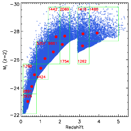
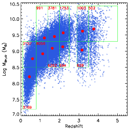
Figure 1.— Distributions of quasars in the redshift-luminosity (left) and redshift-virial mass (right) planes, for our uniform quasar sample. The superposed grids indicate the subsamples we use to explore dependences of clustering strength on luminosity and virial BH mass. In each bin, the number of quasars is marked, and the red filled circle marks the location of the median value. Note that these grids avoid straddling the redshift deserts at $z\sim 2.7$ and $z\sim 3.5$ due to quasar selection inefficiency (see text).

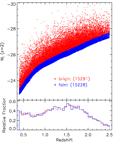
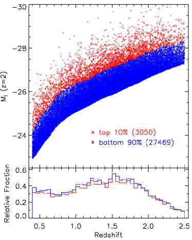
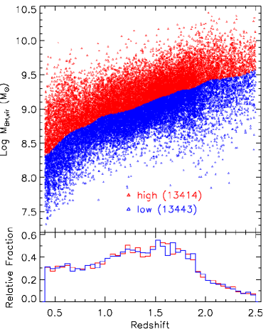
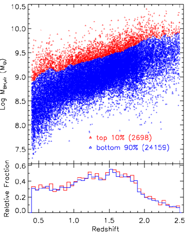
Figure 2.— Sample divisions at median and $10\%$ highest luminosities (upper panels) and virial masses (bottom panels), in the redshift range $0.4\leq z\leq 2.5$. In the bottom of each panel we show the normalized redshift distributions for each subsample. The similarity of their redshift distributions allows a fair comparison of their relative clustering strength.

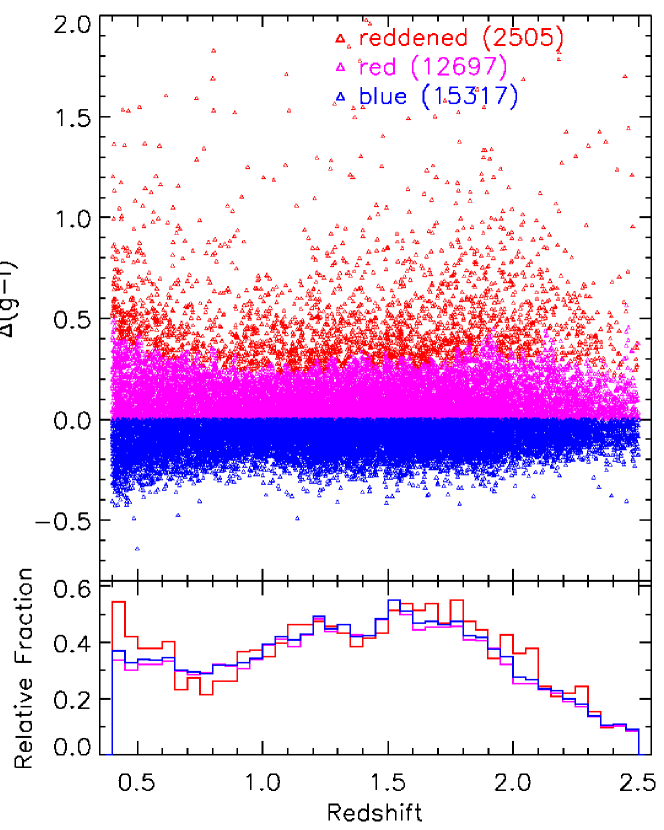
Figure 3.— Sample divisions using quasar color excess (Richards et al. 2003), in the redshift range $0.4\leq z\leq 2.5$ (see §2.1). In the bottom panel we show the normalized redshift distributions for each subsamples. The similarity of their redshift distributions allows a fair comparison of their relative clustering strength.

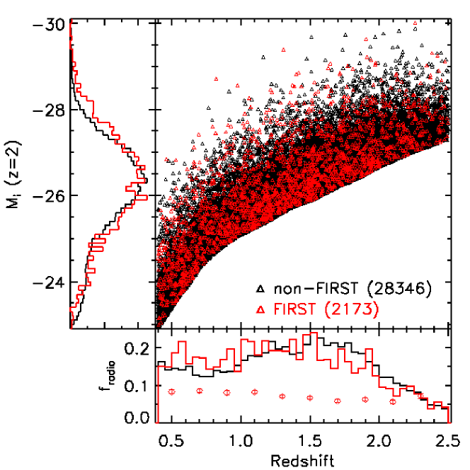
Figure 4.— FIRST detected and undetected quasars. Histograms show the distributions in redshift and optical luminosity for the two samples. The radio fraction as a function of redshift is shown as open symbols in the bottom panel.

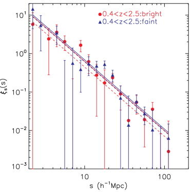
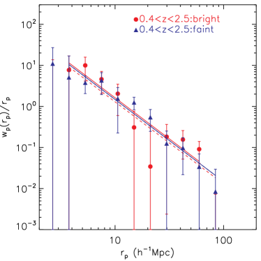
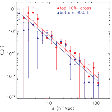
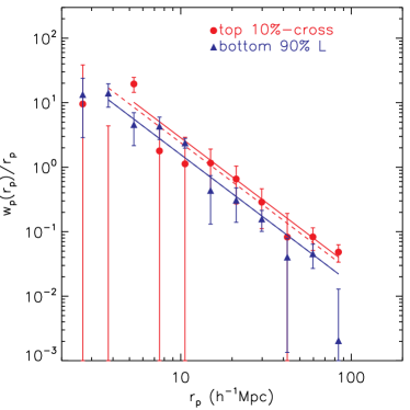
Figure 5.— Luminosity dependence of quasar clustering, using the bright/faint samples (top panels) or the top $10\%$ luminosity divided samples (bottom panels), with $0.4\leq z\leq 2.5$ as defined in §2.1. For the top $10\%$ most luminous quasars we have cross-correlated them with the remaining $90\%$ quasars. Solid and dashed lines are the best-fit power-law models excluding and including negative data bins in the fits, respectively (see text for details). Left: redshift space correlation function. right: projected correlation function. No appreciable difference in the clustering strength is observed for the median luminosity division. But the most luminous quasars show appreciably stronger clustering than the rest of the quasars.

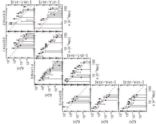
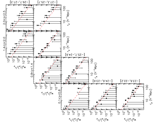
Figure 6.— Correlation functions in each redshift-luminosity bin as defined in the left panel of Fig. 1. The redshift ranges are marked on the top of each column and the luminosity [$M_{i}(z=2)$] ranges are marked on the right of each row. Left: redshift space correlation function. Right: projected correlation function. In each panel, the dashed line is a power law model of $\xi_{s}(s)=(s/6.5\ h^{-1}{\rm Mpc})^{-1.8}$ or $\xi(r)=(r/6.5\ h^{-1}{\rm Mpc})^{-2}$, drawn to guide the eye. No appreciable difference is seen in each luminosity bin at fixed redshift, due to large error bars in the correlation functions caused by small sample sizes.

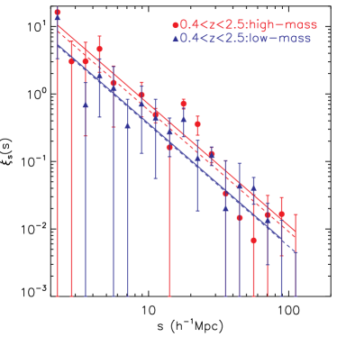
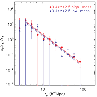
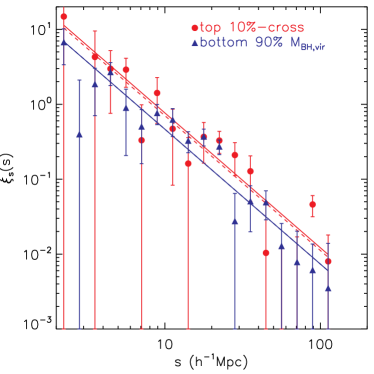
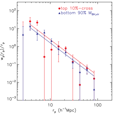
Figure 7.— Virial mass dependence of quasar clustering, using the high/low-mass samples (upper panels) or the top $10\%$ virial mass divided samples (lower panels) as defined in §2.1. Solid and dashed lines are the best-fit power-law models excluding and including negative data bins in the fits, respectively. Left: redshift space correlation. Right: projected correlation function. The high/low-mass samples are consistent with no difference in clustering strength given the measurement errors. However, the most massive quasars are more strongly clustered than are the rest of the quasars.

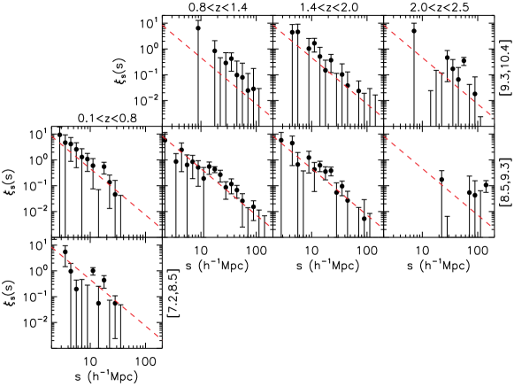
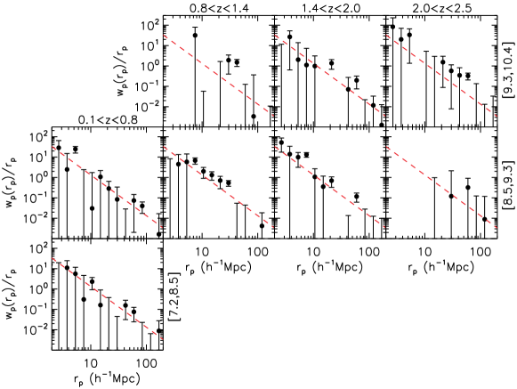
Figure 8.— Correlation functions in each redshift-virial mass bin as defined in the right panel of Fig. 1. luminosity bin as defined in the left panel of Fig. 1. The redshift ranges are marked on the top of each column and the virial mass $(\log M_{\rm BH,vir}/M_{\odot})$ ranges are marked on the right of each row. Upper: redshift space correlation function. Bottom: projected correlation function. In each panel, the dashed line is a power law model of $\xi_{s}(s)=(s/6.5\ h^{-1}{\rm Mpc})^{-1.8}$ or $\xi(r)=(r/6.5\ h^{-1}{\rm Mpc})^{-2}$, drawn to guide the eye. No appreciable difference is observed at fixed redshift, due to the large uncertainties in the correlation functions.

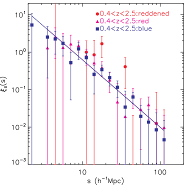
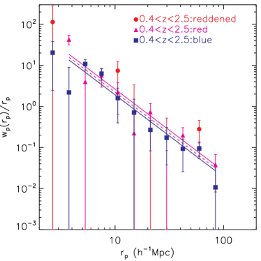
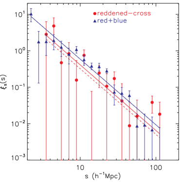
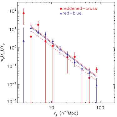
Figure 9.— Clustering of blue, red and reddened quasars, using the samples defined in §2.1. Solid and dashed lines are the best-fit power-law models excluding and including negative data bins in the fits, respectively. Left panels: redshift space correlation functions. Right panels: projected correlation functions. In the upper two panels we show the auto-correlation functions for the three samples; there is no appreciable difference between the red and blue quasar samples. The auto-correlation function of the reddened sample is too noisy to be useful. In the bottom panels, we show the auto-correlation functions for the red$+$blue sample and the cross-correlation of the reddened sample with the red$+$blue sample. Again no discernible difference is observed given the uncertainty levels in the CF measurements.

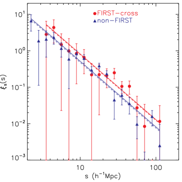
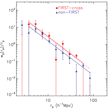
Figure 10.— Clustering results for the radio-loud and radio-quiet samples as defined in §2.1. Solid and dashed lines are the best-fit power-law models excluding and including negative data bins in the fits, respectively. Left: redshift space correlation function. Right: projected correlation function. The cross-correlation function of the radio-loud sample with the radio-quiet sample is larger than the auto correlation function of the latter sample, as shown in both panels.

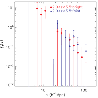
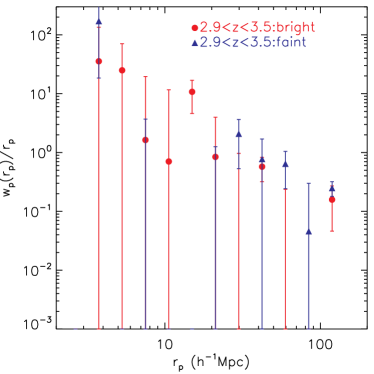
Figure 11.— Binned CFs for the two high-$z$ luminosity bins. Left: redshift space correlation function. Right: projected correlation function. Despite the absence of detectable correlation for the fainter sample (triangles) at $r\lesssim 20\ h^{-1}$Mpc, which may be caused by systematic effects (see the text), there is no appreciable difference at large scales ($r\gtrsim 20\ h^{-1}$Mpc) for the two samples, although the error bars are large.

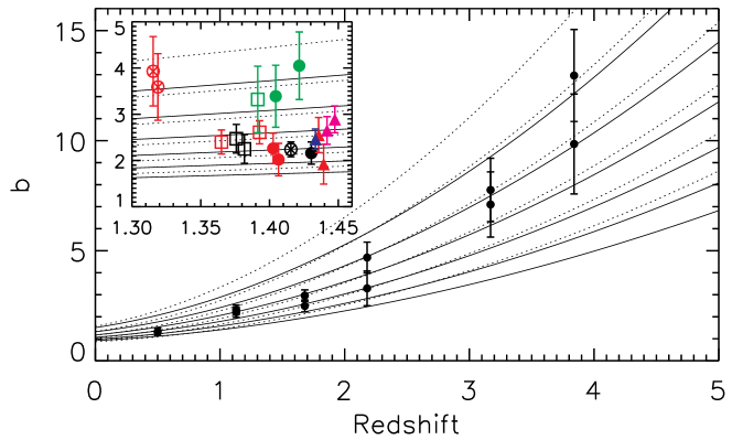
Figure 12.— Measured quasar bias factors for various samples. The filled circles in the main frame are results for all quasars within each redshift bin (no magnitude cut) and results both with and without negative data points in the fitting procedure are shown. The solid and dotted lines are halo bias factor evolution for fixed halo mass (from bottom to top) $M_{\rm halo}=5\times 10^{11},\ 1\times 10^{12},\ 2\times 10^{12},\ 4\times 10^{12},\ 8\times 10^{12},\ 1.6\times 10^{13}\ h^{-1}M_{\odot}$ using the Sheth et al. (2001) and Jing (1998) fitting formulae respectively. The Jing (1998) formula generally gives larger halo bias than the Sheth et al. (2001) formula for the same halo mass. In the inset we show the quasar biases for our $0.4<z<2.5$ assembly samples divided by luminosity (filled circles; black for faint quasars, red for bright quasars, and green for the brightest quasars), virial mass (open squares; black for low-mass, red for high-mass and green for the most massive quasars), color (filled triangles, blue for blue quasars, magenta for red quasars and red for reddened quasars), and radio detection (circles with x; black for FIRST-undetected quasars and red for FIRST-detected quasars). Their median redshifts have been shuffled to avoid clustering in the plot.

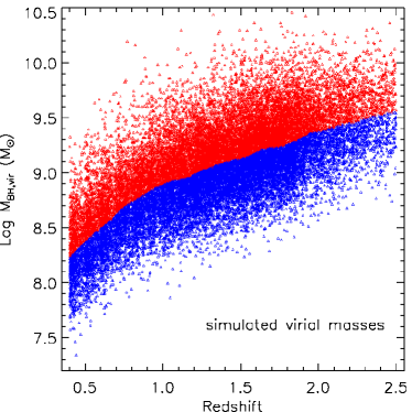
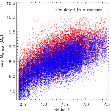
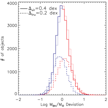
Figure 13.— Simulated virial (left) and true (middle) BH masses. In addition to the Malmquist-type bias between the virial and the true BH masses (e.g., Shen et al. 2008b), the two samples divided using the median virial BH masses overlap substantially in their true masses. In the right panel we show the distributions of BH masses relative to the median values. The solid and dotted histograms show the distributions of deviation from the median value (which varies with redshift) for observed and simulated virial BH masses, which are in reasonable agreement. The dashed histograms show the distributions of simulated true BH masses of the two samples divided by the median virial BH masses. The median difference in the two samples are 0.4 dex in virial BH masses and 0.2 dex in true BH masses.

References

- (1) Abazajian, K., et al. 2003, AJ, 126, 2081 (DR1)
- (2) Abazajian, K., et al. 2008, ApJS, submitted (DR7)
- (3) Adelberger, K. L., & Steidel, C. C. 2005, ApJ, 627, L1
- (4) Adelman-McCarthy, J. K., et al. 2007, ApJS, 172, 634 (DR5)
- (5) Baes, M., Buyle, P., Hau, G. K. T., & Dejonghe, H. 2003, MNRAS, 341L, 44
- (6) Bardeen, J., Bond, J. R., Kaiser, N. & Szalay, A. S. 1986, ApJ, 304, 15
- (7) Basilakos, S., Plionis, M., & Ragone-Figueroa, C. 2008, ApJ, 678, 627
- (8) Blanton, M. R., et al. 2003, AJ, 125, 2276
- (9) Coil, A., Hennawi, J. F., Newman, J. A., Cooper, M. C., & Davis, M. 2007, ApJ, 654, 115
- (10) Cole, S., & Kaiser, N. 1989, MNRAS, 237, 1127
- (11) Constantin, A., & Vogeley, M. S. 2006, ApJ, 650, 727
- (12) Courteau, S., McDonald, M., Widrow, L. M., & Holtzman, J. 2007, ApJ, 655, L21
- (13) Croft, R. A. C., Dalton, G. B., Efstathiou, G., Sutherland, W. J., & Maddox, S. J. 1997, MNRAS, 291, 305
- (14) Croton, D. J., et al. 2006, MNRAS, 365, 11
- (15) Croton, D. J. 2008, MNRAS, submitted
- (16) Croom, S. M., et al. 2004, MNRAS, 349, 1379
- (17) Croom, S. M., et al. 2005, MNRAS, 356, 415
- (18) Croom, S. M., et al. 2008, MNRAS, in press
- (19) da Ângela, J., et al. 2005, MNRAS, 360, 1040
- (20) da Ângela, J., et al. 2008, MNRAS, 383, 565
- (21) Davis, M., & Peebles, P. J. E. 1983, ApJ, 267, 465
- (22) Di Matteo, T., Springel, V., & Hernquist, L. 2005, Nature, 433, 604
- (23) Eisenstein, D. J., & Hu, W. 1999, ApJ, 511, 5
- (24) Fan, X. 1999, AJ, 117, 2528
- (25) Ferrarese, L. 2002, ApJ, 578, 90
- (26) Fukugita, M., et al. 1996, AJ, 111, 1748
- (27) Furlanetto, S. R., & Kamionkowski, M. 2006, MNRAS, 366, 529
- (28) Gao, L., Springel, V., & White, S. D. M. 2005, MNRAS, 363, L66
- (29) Gunn, J. E., et al. 1998, AJ, 116, 3040
- (30) Gunn, J. E., et al. 2006, AJ, 131, 2332
- (31) Haiman, Z., & Hui, L. 2001, ApJ, 547, 27
- (32) Hamilton, A. J. S. 1993, ApJ, 417, 19
- (33) Hamilton, A. J. S., & Tegmark, M. 2004, MNRAS, 349, 115
- (34) Hennawi, J., et al. 2006, AJ, 131, 1
- (35) Ho, L. C. 2007, ApJ, 668, 94
- (36) Hopkins, P. F., et al. 2004, AJ, 128, 1112
- (37) Hopkins, P. F., Hernquist, L., Martini, P., Cox, J., Robertson, B., Di Matteo, T., & Springel, V. 2005, ApJ, 625, L71
- (38) Hopkins, P. F., Hernquist, L., Cox, T. J., Di Matteo, T., Robertson, B., & Springel, V. 2006, ApJS, 163, 1
- (39) Hopkins, P. F., Lidz, A., Hernquist, L., Coil, A. L., Myers, A. D., Cox, T. J. & Spergel, D. N. 2007, ApJ, 662, 110
- (40) Ivezić, Z., et al. 2004, AN, 325, 583
- (41) Jiang, L., et al. 2007, ApJ, 656, 680
- (42) Jing, Y. P. 1998, ApJ, 503, L9
- (43) Kaiser, N. 1984, ApJ, 284, L9
- (44) Kaiser, N., et al. 2002, Proc. SPIE, 4836, 154
- (45) Kauffmann, G., & Haehnelt, M. 2000, MNRAS, 311, 576
- (46) King, A. 2003, ApJ, 596, L27
- (47) Kollmeier, J. A. et al. 2006, ApJ, 648, 128
- (48) Kormendy, J., & Richstone, D. 1995, ARA&A, 33, 581
- (49) Landy, S. D., & Szalay, A. S. 1993, ApJ, 412, 64
- (50) Li, C., et al. 2006, MNRAS, 373, 457
- (51) Lidz, A., Hopkins, P. F., Cox, T. J., Hernquist, L., & Robertson, B. 2006, ApJ, 641, 41
- (52) Lin, Y.-T., et al. 2008, in preparation
- (53) Lupton, R., Gunn, J. E., Ivezić, Z., Knapp, G. R., & Kent, S. 2001, ASP Conference Proceedings, 238, 269
- (54) Lynden-Bell, D. 1969, Nature, 223, 690
- (55) Magorrian, J., et al. 1998, AJ, 115, 2285
- (56) Martini, P., & Weinberg, D. H. 2001, ApJ, 547, 12
- (57) Mandelbaum, R., Li, C., Kauffmann, G., & White, S. D. M. 2008, MNRAS, submitted, arXiv:0806.4089
- (58) McLure, R. J., & Jarvis, M. J. 2002, MNRAS, 337, 109
- (59) Mo, H. J., & White, S. D. M. 1996, MNRAS, 282, 347
- (60) Myers, A. D., et al. 2006, ApJ, 638, 622
- (61) Myers, A. D., et al. 2007a, ApJ, 658, 85
- (62) Myers, A. D., et al. 2007b, ApJ, 658, 99
- (63) Myers, A. D., et al. 2008, ApJ, 678, 635
- (64) Padmanabhan, N., et al. 2007, ApJ, 378, 852
- (65) Padmanabhan, N., White, M., Norberg, P., & Porciani, C. 2008, MNRAS, submitted, arXiv:0802.2105
- (66) Pier, J. R., et al. 2003, AJ, 125, 1559
- (67) Porciani, C., Magliocchetti, M., & Norberg, P. 2004, MNRAS, 355, 1010
- (68) Porciani, C., Norberg, P. 2006, MNRAS, 371, 1824
- (69) Reichard, T. A., et al. 2003, AJ, 125, 1711
- (70) Richards, G. T., et al. 2002, AJ, 123, 2945
- (71) Richards, G. T., et al. 2003, AJ, 126, 1131
- (72) Richards, G. T., et al. 2006, AJ, 131, 2766
- (73) Richstone, D., et al. 1998, Nature, 395, 14
- (74) Ross, N. P., et al. 2008, ApJ, submitted
- (75) Salpeter, E. E. 1964, ApJ, 140, 796
- (76) Schlegel, D. J., Finkbeiner, D. P., & Davis, M. 1998, ApJ, 500, 525
- (77) Schlegel, D. J., et al. 2007, BAAS, 39, 966
- (78) Schneider, D. P., et al. 2007, AJ, 134, 102
- (79) Shankar, F., Crocce, M., Miralda-Escudeé, J., Fosalba, P. & Weinberg, D. H. 2008b, ApJ, submitted, arXiv:0810.4919
- (80) Shankar, F., Weinberg, D. H., & Miralda-Escudé, J. 2008a, ApJ, in press, arXiv:0710.4488
- (81) Shen, Y., et al. 2007a, AJ, 133, 2222
- (82) Shen, Y., Mulchaey, J. S., Raychaudhury, S., Rasmussen, J., & Ponman, T. J. 2007b, ApJ, 654, L115
- (83) Shen, Y., Strauss, M. A., Hall, P. B., Schneider, D. P., York, D. G., & Bahcall, N. A. 2008a, ApJ, 677, 858
- (84) Shen, Y., Greene, J. E., Strauss, M. A., Richards, G. T., & Schneider, D. P. 2008b, ApJ, 680, 169
- (85) Shen, J., Vanden Berk, D. E., Schneider, D. P., & Hall, P. B. 2008c, AJ, 135, 928
- (86) Sheth, R. K., & Tormen, G. 1999, MNRAS, 308, 119
- (87) Sheth, R. K., Mo, H. J., & Tormen, G. 2001, MNRAS, 323, 1
- (88) Silk, J., & Rees, M. J. 1998, A&A, 331, L1
- (89) Smith, J. A., et al. 2002, AJ, 123, 2121
- (90) Spergel, D. N., et al. 2007, ApJS, 170, 377
- (91) Stephens, A. W., Schneider, D. P., Schmidt, M., Gunn, J. E., & Weinberg, D. H. 1997, AJ, 114, 41
- (92) Stoughton, C., et al. 2002, AJ, 123, 485
- (93) Tinker, J. L., Weinberg, D. H., Zheng, Z., & Zehavi, I. 2005, ApJ, 631, 41
- (94) Tremaine, S., et al. 2002, ApJ, 574, 740
- (95) Tucker, D. L., et al. 2006, AN, 327, 821
- (96) Vestergaard, M., & Peterson, B. M. 2006, ApJ, 641, 689
- (97) Wake, D. A., Croom, S. M., Sadler, E. M., & Johnston, H. M. 2008, MNRAS, in press, arXiv:0810.1050
- (98) Wechsler, R. H., Zentner, A. R., Bullock, J. S., Kravtsov, A. V., & Allgood, B. 2006, ApJ, 652, 71
- (99) Wetzel, A. R., Cohn, J. D., White, M., Holz, D. E., & Warren, M. S. 2007, ApJ, 656, 139
- (100) White, M., Martini, P., & Cohn, J. D. 2008, MNRAS, 390, 1179
- (101) Wyithe, J. S. B., & Loeb, A. 2002, ApJ, 581, 886
- (102) Wyithe, J. S. B., & Loeb, A. 2003, ApJ, 595, 614
- (103) Wyithe, J. S. B., & Loeb, A. 2008, MNRAS, submitted, arXiv:0810.3455
- (104) York, D. G., et al. 2000, AJ, 120, 1579
- (105) Zehavi, I., et al. 2005, ApJ, 630, 1
- (106) Zel’dovich, Y. B., & Novikov, I. D. 1964, Dokl. Akad. Nauk SSSR, 158, 811