Forward $\bar{p}d$ elastic scattering and total spin-dependent $\bar{p}d$ cross sections at intermediate energies

Abstract

Spin-dependent total ${\bar{p}}d$ cross sections are considered using the optical theorem. For this aim the full spin dependence of the forward ${\bar{p}}d$ elastic scattering amplitude is considered in a model independent way. The single-scattering approximation is used to relate this amplitude to the elementary amplitudes of $\bar{p}p$ and $\bar{p}n$ scattering and the deuteron formfactor. A formalism allowing to take into account Coulomb-nuclear interference effects in polarized $\bar{p}d$ cross sections is developed. Numerical calculations for the polarized total ${\bar{p}}d$ cross sections are performed at beam energies 20-300 MeV using the $\bar{N}N$ interaction models developed by the Jülich group. Double-scattering effects are estimated within the Glauber approach and found to be in the order of 10 - 20 %. Existing experimental data on differential $\bar{p}d$ cross sections are in good agreement with the performed Glauber calculations. It is found that for the used ${\bar{N}}N$ models the total longitudinal and transversal ${\bar{p}}d$ cross sections are comparable in absolute value to those for ${\bar{p}}p$ scattering.

I Introduction

Recently the PAX collaboration was formed PAX with the aim to measure the proton transversity in the interaction of polarized antiprotons with protons at the future FAIR facility in Darmstadt. In order to produce an intense beam of polarized antiprotons, the collaboration is going to use antiproton elastic scattering off a polarized hydrogen target (¹H) in a storage ring Rathmann . The basic idea is connected to the result of the FILTEX experiment FILTEX , where a sizeable effect of polarization buildup was achieved in a storage ring by scattering of unpolarized protons off a polarized hydrogen atoms at low beam energies of 23 MeV.

According to recent theoretical analyses MS ; NNNP ; NNNP1 ; NNNP2 the polarization effect observed in Ref. FILTEX has to be interpreted in such a way that solely the spin dependence of the hadronic (proton-proton) interaction provides the spin-filtering mechanism, i.e. is responsible for different rates of removal of protons from the ring for different initial polarization states. In other words MS ; NNNP , proton scattering on the polarized electrons of hydrogen atoms cannot provide a sizeable effect of polarization buildup, as it was assumed before HOM . Indeed, the maximal scattering angle in this process, $\theta_{max}=m_{e}/m_{p}=0.5$ mrad, is less than the beam acceptance angle $\theta_{acc}$, which is defined so that for scattering at smaller angle $\theta<\theta_{acc}$ the projectile remains in the beam. For this case, the beam-into-beam scattering kinematics of this process in a storage ring allows the proton polarization buildup only due to spin-flip transitions between the initial and final spin states of the beam proton MS . Furthermore, since the Coulomb interaction between the protons and electrons is spin-independent it cannot provide spin-flip transitions and, consequently, does not contribute to the polarization buildup. The same argument, obviously, is valid in case of antiproton scattering off a hydrogen target. Therefore, the authors of Ref. MS concluded that only the hadronic interaction can be used to produce polarized antiprotons on the basis of the spin-filtering mechanism.

In contrast to the $NN$ case, the spin-dependent part of the $\bar{p}N$ interaction is poorly known experimentally at present. Therefore, to investigate the polarization buildup mechanism in $\bar{p}~{}^{1}$H scattering a new experiment is planned at CERN AD . The stored antiprotons will be scattered off a polarized ¹H target in that experiment AD and the polarization of the antiproton beam will be measured at intermediate energies. Some theoretical estimations DmitrievMS of the expected polarization effects were already performed employing a specific model of the $\bar{p}p$ interaction.

In this context, it is interesting and useful to explore other hadronic reactions as possible source for the antiproton polarization buildup too. Therefore, in the present work we study polarization effects in antiproton-deuteron (${\bar{p}}d$) scattering for beam energies up to 300 MeV. Besides the issue of polarization buildup for antiprotons, $\bar{p}$ scattering on a polarized deuteron, if it will be studied experimentally, can be also used as a test for our present knowledge of the ${\bar{p}}n$ and ${\bar{p}}p$ interactions. Our investigation is based on the Glauber-Sitenko theory for ${\bar{p}}d$ scattering and it utilizes the ${\bar{N}}N$ interaction models developed by the Jülich group Hippchen ; Hippchen1 ; Mull as input for the elementary amplitudes. Since there are data on (unpolarized) total and differential $\bar{p}d$ cross sections in the considered energy range we can examine the reliability of the Glauber approach via a direct comparison of our results to experimental information. In addition we also present results for polarization effects for the $\bar{N}N$ system itself. With the $\bar{N}N$ potentials developed by the Jülich group we have conceptually rather different models at our disposal than the one used in Ref. DmitrievMS and it will be instructive to see and compare the corresponding predictions. Moreover, we consider here the ${\bar{p}}p$ as well as the ${\bar{p}}n$ case.

Let us mention here for completeness that very recently new QED calculations for polarization transfer in proton-electron (and antiproton-positron) elastic scattering were performed Arenhoevel . These calculations predict very large polarization transfer from polarized electrons (positrons) to unpolarized protons (antiprotons) in elastic proton-electron (antiproton-positron) scattering at low beam energies, less than 20 keV Arenhoevel . On this basis new sources for polarized antiprotons are under discussion Walcher . On the other hand, according to a calculation presented in Ref. MSS , the effect of polarization buildup is negligible in this reaction, even at small relative velocites. A recent measurement performed at COSY Frankpc intends to explore this method. Finally, another method for buildup of polarized antiprotons at high energies, based on production of ${\bar{\Lambda}}(1115)$ and its subsequentional decay ${\bar{\Lambda}}\to\pi^{+}+\bar{p}$, has been proposed in Ref. Nurushev .

The paper is structured in the following way. In the next section we consider the spin structure of the total ${\bar{p}}d$ cross section using the optical theorem. In Sect. III expressions for the forward ${\bar{p}}d$ elastic scattering amplitude are derived in the impulse approximation and the formalism for the polarized total $\bar{p}d$ cross sections is developed. The formalism for calculating the Coulomb-nuclear interference cross sections is presented in Sect. IV. The technical details for evaluating the Coulomb-hadronic interference cross sections for $\bar{p}d$ elastic scattering are summarized in Appendix A. The $\bar{p}N$ interaction model of the Jülich group is briefly reviewed in Sect. V. The amplitudes of this model are used as input for our ${\bar{p}}d$ calculations. We also provide and discuss results for spin-dependent cross sections in the $\bar{p}p$ as well as $\bar{p}n$ channels. Numerical results for the ${\bar{p}}d$ reaction are presented and discussed in section VI. A short summary is provided in the last section.

II Phenomenology of the spin dependence of the total $\bar{p}d$ cross section

Let us first consider only the purely hadronic part of the reaction amplitude. The modifications due to the presence of the Coulomb interaction will be discussed in Sect. IV. We use the optical theorem to derive the formalism for the total spin dependent $\bar{p}d$ cross sections. According to phillips one has

$$Im\frac{Tr(\hat{\rho}_{i}\hat{F}(0))}{Tr\hat{\rho}_{i}}=\frac{k_{\bar{p}d}}{4\pi}\sigma_{i},$$ (1)

where $\hat{F}(0)$ is the transition operator for $\bar{p}d$ elastic scattering at the angle $\theta=0$, $\rho_{i}$ is the initial spin-density matrix, $\sigma_{i}$ is the total cross section depending on the density matrix $\rho_{i}$, and $k_{\bar{p}d}$ is the momentum in the center-of-mass system (cms).

The spin dependence of the amplitude of the $\bar{p}d$ elastic scattering is the same as for the $pd$ elastic scattering. For collinear kinematics it contains four independent terms rekalo and can be written as uzepan98

$$\hat{F}_{\alpha\beta}(0)=g_{1}\delta_{\alpha\beta}+(g_{2}-g_{1})m_{\alpha}m_{\beta}+ig_{3}{\hat{\sigma}}_{i}\epsilon_{\alpha\beta i}+i(g_{4}-g_{3}){\hat{\sigma}}_{i}m_{i}m_{j}\epsilon_{\alpha\beta j},$$ (2)

where $\hat{\sigma}_{i}$ ($i=x,y,z$) are the Pauli spin matrices, $\epsilon_{\alpha\beta\gamma}$ is the fully antisymmetric tensor, $m_{\alpha}$ are the Cartesian components of a unit vector ${\bf m}$ pointing along the beam momentum, and $g_{i}$ $(i=1,\dots,4)$ are complex numbers determined by the dynamics of the reaction. Let us put the $z$ axis along the vector ${\bf m}$, so that ${\bf m}=(m_{x},m_{y},m_{z})=(0,0,1)$. The $\bar{p}d$ elastic scattering amplitude is obtained by sandwiching the operator $\hat{F}_{\alpha\beta}$ between antiproton and deuteron spin states,

$$F_{\mu\lambda}^{\mu^{\prime}\lambda^{\prime}}\equiv<\mu^{\prime}\lambda^{\prime}|{\hat{F}}|\mu\lambda>=\phi^{+}_{\mu^{\prime}}e_{\beta}^{(\lambda^{\prime})^{*}}{\hat{F}}_{\alpha\beta}e_{\alpha}^{(\lambda)}\phi_{\mu},$$ (3)

where $\phi_{\mu}$ ($\phi_{\mu^{\prime}}$) is the Pauli spinor for the initial (final) antiproton with the spin projection $\mu$ ($\mu\prime$) and $e_{\alpha}^{(\lambda)}$ ($e_{\beta}^{(\lambda^{\prime})}$) is the polarization vector of the initial (final) deuteron with the spin projection $\lambda$ ($\lambda^{\prime})$.

When choosing different initial polarization states in Eq. (1), described by the product of the spin density matrices of the antiproton $\rho^{\bar{p}}$ and the deuteron ${\hat{\rho}^{d}}$, $\rho=\rho^{\bar{p}}\rho^{d}$, one can derive from Eqs. (1) and (2) different total spin-dependent cross sections in terms of the forward amplitudes $g_{i}$. For example, for unpolarized antiprotons and unpolarized deuterons one has $\rho=\frac{1}{2}\times\frac{1}{3}$, and one finds from Eq. (1) the unpolarized total cross section to be

$$\sigma_{0}=\frac{2\pi}{k_{\bar{p}d}}Im(g_{1}+g_{2})\ .$$ (4)

In general the spin density matrices are

$$\rho^{\bar{p}}=\frac{1}{2}(1+{\bf P}^{\bar{p}}{\hat{{\mbox{\boldmath$\sigma$}}}})$$ (5)

for the antiproton and

$$\rho^{d}=\frac{1}{3}+\frac{1}{2}S_{j}P_{j}^{d}+\frac{1}{9}S_{jk}P_{jk}^{d}$$ (6)

for the deuteron. Here $S_{j}$ is the spin-1 operator, ${P}_{j}^{d}$ and $P_{jk}^{d}$ $(j,k=x,y,z)$ are the vector and tensor polarizations of the deuteron, and $S_{jk}=(S_{j}S_{k}+S_{k}S_{j}-\frac{4}{3}\delta_{jk})$ is the spin-tensor operator.

Using Eqs. (2), (5) and (6) one can find from Eq. (1),

$$Tr\{\rho^{\bar{p}}\times\rho^{d}{\hat{F}}(0)\}=\frac{1}{2}(g_{1}+g_{2})+P_{x}^{\bar{p}}P_{x}^{d}g_{3}+P_{y}^{\bar{p}}P_{y}^{d}g_{3}+P_{z}^{\bar{p}}P_{z}^{d}g_{4}+$$

$$+\frac{1}{9}P_{xx}^{d}(g_{1}-g_{2})+\frac{1}{9}P_{yy}^{d}(g_{1}-g_{2})+\frac{5}{18}P_{zz}^{d}(g_{1}-g_{2}).$$ (7)

As seen from this formula, if the initial antiproton is polarized with the polarization vector ${\bf P}^{\bar{p}}$ and the deuteron has the polarization vector ${\bf P}^{d}$, then non-zero terms $\sigma_{i}$ arise in the right-hand side of Eq. (1) for parallel (or antiparallel) orientation of the vectors ${\bf P}^{\bar{p}}$ and ${\bf P}^{d}$. For the tensor polarization of the deuteron only the diagonal components of the polarization tensor $P_{xx}^{d}$, $P_{yy}^{d}$ and $P_{zz}^{d}$ are connected with non-zero total cross section. The cross sections associated with $P_{xx}^{d}$ and $P_{yy}^{d}$ are the same and determined by $\frac{1}{9}(g_{1}-g_{2})$, whereas the cross section connected with the $P_{zz}^{d}$ component is given by $\frac{5}{18}(g_{1}-g_{2})$. Taking into account the relation $P_{xx}^{d}+P_{yy}^{d}+P_{zz}^{d}=0$, one can find from Eq. (II) that the total tensor cross section can be connected only with the $P_{zz}^{d}$ component.

All other combinations of polarizations of the antiproton and/or deuteron, namely, polarized antiproton, vector-polarized deuteron, and polarized antiproton – tensor-polarized deuteron, give zero contribution to the total cross section due to parity conservation.

Summarizing the above results, the total polarized ${\bar{p}}d$ section can be written as

$$\sigma=\sigma_{0}+\sigma_{1}{\bf P}^{\bar{p}}\cdot{\bf P}^{d}+\sigma_{2}({\bf P}^{\bar{p}}\cdot{\bf m})({\bf P}^{d}\cdot{\bf m})+\sigma_{3}P_{zz}^{d},$$ (8)

where $\sigma_{0}$ is given by Eq. (4), and the other coefficients are:

$$\sigma_{1} = \frac{4\pi}{k_{\bar{p}d}}Img_{3},$$

$$\sigma_{2} = \frac{4\pi}{k_{\bar{p}d}}Im(g_{4}-g_{3}),$$

$$\sigma_{3} = \frac{4\pi}{k_{\bar{p}d}}Im\frac{(g_{1}-g_{2})}{6}.$$ (9)

One can find from Eq. (8) that only the cross sections $\sigma_{1}$ and $\sigma_{2}$ are connected with the spin-filtering mechanism and, therefore, determine the rate of the polarization buildup in the scattering of unpolarized antiprotons off polarized deuterons. (More precisely, the rate of polarization buildup is determined by the ratio $\sigma_{1}/\sigma_{0}$ for transversal polarization and by $(\sigma_{2}-\sigma_{1})/\sigma_{0}$ for longitudinal polarization of target and beam in the storage ring.) The tensor cross section $\sigma_{3}$ is not connected with the polarization of the beam and, therefore, is not relevant for the spin-filtering. However, this cross section, as well as the unpolarized cross section $\sigma_{0}$, determines the lifetime of the beam. When changing the sign of the tensor polarization $P_{zz}^{d}$, one may change the beam lifetime.

III $\bar{p}d$ elastic scattering at forward angles

III.1 Glauber theory

Within the Glauber theory the amplitudes for the elastic ($\bar{p}d\to\bar{p}d$) and breakup ($\bar{p}d\to\bar{p}np$) reactions are given by the following matrix element

$$F_{if}({\bf q})=<f|F({\bf q},{\bf s})|i>,$$ (10)

calculated between definite initial $|i>$ and final $|f>$ states of the two-nucleon system. Here the transition operator is

$$F({\bf q},{\bf s})=\exp{(\frac{1}{2}i{\bf q}\cdot{\bf s})}f_{\bar{p}p}({\bf q})+\exp{(-\frac{1}{2}i{\bf q}\cdot{\bf s})}f_{\bar{p}n}({\bf q})+\frac{i}{2\pi k_{\bar{p}d}}\int\exp{(i{\bf q}^{\prime}\cdot{\bf s})}f_{\bar{p}n}({\bf q^{\prime}}+\frac{1}{2}{\bf q})f_{\bar{p}p}(-{\bf q^{\prime}}+\frac{1}{2}{\bf q})d^{2}{\bf q}^{\prime}.$$ (11)

In Eqs. (10) and (11) ${\bf q}$ is the transferred momentum, ${\bf s}$ is the impact parameter, and $f_{\bar{p}N}({\bf q})$ ($N=p,n$) is the $\bar{p}N$ scattering amplitude. The amplitude of elastic $\bar{p}d$ scattering can be expressed via the elastic form factor of the deuteron, $S({\bf q})$, and the elementary amplitudes of $\bar{p}N$ scattering. The differential scattering cross section for elastic ($\bar{p}d\to\bar{p}d$) plus inelastic ($\bar{p}d\to\bar{p}pn$) scattering is calculated within the closure approximation FrancoGlauber . That allows one to express the scattering cross section via $f_{\bar{p}N}({\bf q})$, $S({\bf q})$ and the deuteron wave function. Since the D-wave component of the deuteron wave function becomes important only in the region of the first diffraction minimum of the differential $\bar{p}d$ cross section mahalabi , we neglect its contribution in the present calculations and take into account only the S-wave component.

As seen from Eq. (11), in the Glauber theory of multiple scattering of hadrons off the deuteron only single-scattering (first two terms on the right-hand side) and double-scattering (third term on the right-hand side) mechanisms contribute to the transition amplitude. In forward direction the single-scattering mechanism dominates. The corrections related to double-scattering effects produce the so-called shadowing effect. As a result, the total unpolarized antiproton-deuteron cross section $\sigma^{\bar{p}d}$ is not equal to the sum of the total $\bar{p}p$ and $\bar{p}n$ cross sections, $\sigma^{\bar{p}p}$ and $\sigma^{\bar{p}n}$, but is given by

$$\sigma^{\bar{p}d}=\sigma^{\bar{p}p}+\sigma^{\bar{p}n}-\delta\sigma^{d},$$ (12)

where $\delta\sigma^{d}$ stands for the corrections due to double-scattering effects.

III.2 Impulse approximation

In the impulse approximation (IA) (or single-scattering approximation) one can present the forward $\bar{p}d$ elastic scattering amplitude in the following form

$$F_{\mu\lambda}^{\mu^{\prime}\lambda^{\prime}}=\frac{m_{d}}{m_{N}}\sqrt{\frac{s_{\bar{p}N}}{s_{\bar{p}d}}}\sum_{\sigma\,\sigma^{\prime}\,\sigma_{N}}<\sigma^{\prime}\mu^{\prime}|f_{\bar{p}N}|\sigma\mu>S_{\lambda\,\lambda^{\prime}}^{\sigma\sigma^{\prime}\sigma_{N}}({\bf Q}=0),$$ (13)

where $<\sigma^{\prime}\mu^{\prime}|f_{\bar{p}N}|\sigma\mu>$ is the $\bar{p}N$ scattering amplitude at zero degree, defined as in Ref. bystricky , $S_{\lambda\,\lambda^{\prime}}^{\sigma\sigma^{\prime}\sigma_{N}}({\bf Q}=0)$ is the elastic form factor of the deuteron at zero transferred momentum ${\bf Q}$, $s_{\bar{p}N}$ ($s_{\bar{p}d}$) is the invariant mass of the $\bar{p}N$ ($\bar{p}d$) system, and $m_{d}$ ($m_{N}$) is the mass of the deuteron (nucleon). The sum in Eq. (13) runs over the $z$ projections of the spin of the nucleon spectator $(\sigma_{N})$, and of the initial ($\sigma$) and recoil ($\sigma^{\prime}$) nucleons inside the deuteron. The transition operator for the $\bar{p}N$ forward scattering amplitude has the form bystricky

$$f_{\bar{p}N}=A_{N}+B_{N}({{\mbox{\boldmath$\sigma$}}}_{1}\cdot{{\mbox{\boldmath$\sigma$}}}_{2})+D_{N}({{\mbox{\boldmath$\sigma$}}}_{1}\cdot{\bf m})({{\mbox{\boldmath$\sigma$}}}_{2}\cdot{\bf m}),$$ (14)

where the matrix ${{\mbox{\boldmath$\sigma$}}}_{1}$ (${{\mbox{\boldmath$\sigma$}}}_{2}$) acts on the spin state of the antiproton (nucleon) and $A_{N}$, $B_{N}$ and $D_{N}$ ($N=p,n$) are complex amplitudes bystricky .

The deuteron elastic form factor at ${\bf Q}=0$ can be written as

$$S_{\lambda\,\lambda^{\prime}}^{\sigma\sigma^{\prime}\sigma_{N}}({\bf Q}=0)=\sum_{l\,m\,M_{S}\,M_{S}^{\prime}}(\frac{1}{2}\sigma\frac{1}{2}\sigma_{N}|1M_{S})(1M_{S}\,l\,m|1\lambda)(\frac{1}{2}\sigma\frac{1}{2}\sigma_{N}|1M_{S})(1M_{S}\,l\,m|1\lambda)(1M_{S}^{\prime}\,l\,m|1\lambda^{\prime})\,P_{l},$$ (15)

where $P_{l}$ is the relative weight of the S-wave ($l=0$) and D-wave $(l=2)$ components of the deuteron wave function with the normalization $P_{0}+P_{2}=1$.

Using Eq. (2) one can find the invariant amplitudes $g_{1},\dots,g_{4}$ from the following transition matrix elements $<\mu^{\prime}\lambda^{\prime}|{\hat{F}}|\mu\lambda>$ of $\bar{p}d$ forward scattering rekalo :

$$<+\frac{1}{2},\phantom{+}0|\hat{F}|+\frac{1}{2},\phantom{+}0> = g_{2}$$

$$<+\frac{1}{2},+1|\hat{F}|+\frac{1}{2},+1> = g_{1}-g_{4},$$

$$<+\frac{1}{2},-1|\hat{F}|+\frac{1}{2},-1> = g_{1}+g_{4},$$

$$<+\frac{1}{2},-1|\hat{F}|-\frac{1}{2},\phantom{+}0> = -\sqrt{2}g_{3}.$$ (16)

On the other hand, using Eqs. (13), (14) and (15), one can express the transition matrix elements in terms of the $\bar{p}N$ scattering amplitudes as

$$<+\frac{1}{2},\phantom{+}0|\hat{F}|+\frac{1}{2},\phantom{+}0> = A\,w,$$

$$<+\frac{1}{2},+1|\hat{F}|+\frac{1}{2},+1> = (A+B+D)\,w,$$

$$<+\frac{1}{2},-1|\hat{F}|+\frac{1}{2},-1> = (A-B-D)\,w,$$

$$<+\frac{1}{2},-1|\hat{F}|-\frac{1}{2},\phantom{+}0> = \sqrt{2}B\,w,$$ (17)

where $A=A_{p}+A_{n}$, $B=B_{p}+B_{n}$, $D=D_{p}+D_{n}$ and

$$w=\frac{m_{d}}{m_{N}}\sqrt{\frac{s_{\bar{p}N}}{s_{\bar{p}d}}}(P_{0}-\frac{1}{2}P_{2}).$$ (18)

From a comparison of Eqs. (III.2) with Eqs. (17) one can find that in the single-scattering approximation the invariant amplitudes can be written as

$$g_{1}=g_{2}=Aw = \phantom{-}\frac{1}{2}\left[M_{1}(0)+M_{3}(0)\right]w,$$

$$g_{3}=-Bw = -\frac{1}{2}M_{2}(0)w,$$

$$g_{4}=-(B+D)w = \phantom{-}\frac{1}{2}\left[M_{1}(0)-M_{3}(0)\right]w.$$ (19)

Here we used the standard relations between the amplitudes $A_{N}$, $B_{N}$, and $D_{N}$ and the helicity amplitudes $M_{i}^{N}$ of $\bar{p}N$ scattering bystricky together with the notation $M_{i}=M_{i}^{p}+M_{i}^{n}$. Utilizing Eqs. (4), (9) and (III.2) the total cross sections are thus

$$\sigma_{0}^{IA} = \frac{2\pi}{k_{\bar{p}d}}Im\left[M_{1}^{p}(0)+M_{3}^{p}(0)+M_{1}^{n}(0)+M_{3}^{n}(0)\right]w=(\sigma_{0}^{\bar{p}p}+\sigma_{0}^{\bar{p}n}){\widetilde{w}},$$

$$\sigma_{1}^{IA} = -\frac{2\pi}{k_{\bar{p}d}}Im\left[M_{2}^{p}(0)+M_{2}^{n}(0)\right]w=-(\sigma_{1}^{\bar{p}p}+\sigma_{1}^{\bar{p}n}){\widetilde{w}},$$

$$\sigma_{2}^{IA} = \frac{2\pi}{k_{\bar{p}d}}Im\left[M_{1}^{p}(0)+M_{2}^{p}(0)-M_{3}^{p}(0)+M_{1}^{n}(0)+M_{2}^{n}(0)-M_{3}^{n}(0)\right]w=-(\sigma_{2}^{\bar{p}p}+\sigma_{2}^{\bar{p}n}){\widetilde{w}},$$

$$\sigma_{3}^{IA} = 0,$$ (20)

where we used the relations bystricky

$$\sigma_{0}^{\bar{p}N} = \frac{2\pi}{k_{\bar{p}N}}Im\left[M_{1}^{N}(0)+M_{3}^{N}(0)\right],$$

$$\sigma_{1}^{\bar{p}N} = \frac{2\pi}{k_{\bar{p}N}}Im\left[M_{2}^{N}(0)\right],$$

$$\sigma_{2}^{\bar{p}N} = -\frac{2\pi}{k_{\bar{p}N}}Im\left[M_{1}^{N}(0)+M_{2}^{N}(0)-M_{3}^{N}(0)\right],$$ (21)

and the fact that the cms momentum in the $\bar{p}N$ system, $k_{\bar{p}N}$, is related to the ${\bar{p}d}$ cms momentum, $k_{\bar{p}d}$, by

$$\frac{k_{\bar{p}d}}{k_{\bar{p}N}}=\frac{m_{d}}{m_{N}}\sqrt{\frac{s_{\bar{p}N}}{s_{\bar{p}d}}}\ ,$$ (22)

for equal ($\bar{p}$) beam energies $T_{lab}$ in the reactions $\bar{p}N$ and $\bar{p}d$. The quantity $\widetilde{w}$ in Eqs. (20) is defined by $\widetilde{w}=P_{0}-\frac{1}{2}P_{2}$.

One can see from Eqs. (20) that in the impulse approximation all total cross sections are additive, i.e. given by the sum of the corresponding cross sections on the proton and neutron. While this result is obvious for the total unpolarized ${\bar{p}d}$ cross section $\sigma_{0}$, it was not expected for the spin-dependent cross sections, especially, in view of the opposite sign of the $\bar{p}d$ cross sections $\sigma_{1}$ and $\sigma_{2}$ with regard to $\sigma_{1}^{\bar{p}N}$ and $\sigma_{2}^{\bar{p}N}$, respectively.

III.3 Shadowing effects

As already mentioned above, the double-scattering mechanism dominates at large scattering angles, while its relative contribution decreases when approaching the scattering angle $\theta=0$. The numerical calculations of the forward amplitude of $\bar{p}d$ elastic scattering, which will be presented below, demonstrate that the inclusion of the double-scattering mechanism reduces the total unpolarized cross section by around 15 % at energies 50-300 MeV as compared to the result obtained within the single-scattering approximation If one adopts the approximaton given in Ref. Alberi then the effects of double-scattering for polarized $\bar{p}d$ cross sections should be likewise around 15-20 % in the energy region in question. Thus, we expect them to be significantly smaller than the variations in the predictions due to the uncertainties in the spin-dependence of the elementary $\bar{p}N$ interaction. Therefore, we do not consider the double-scattering effects on the spin-dependent cross sections in the present investigation, which anyway has an exploratory character. Note that an accurate evaluation of the contribution of double-scattering effects to polarized cross sections requires to consider the D-wave component of the deuteron as well as the angular dependence of all (ten) $\bar{p}N$ helicity amplitudes Alberi1 and is therefore rather tedious.

IV Coulomb-nuclear interference

The total polarized cross sections including the Coulomb interaction can be written as the sum of the purely hadronic contributions $\sigma_{i}^{h}$, the Coulomb-nuclear interference terms $\sigma^{int}_{i}$ and the pure Coulomb contribution $\sigma^{C}_{i}$:

$$\sigma_{0} = \sigma_{0}^{h}+\sigma_{0}^{int}+\sigma_{0}^{C},$$

$$\sigma_{1} = \sigma_{1}^{h}+\sigma_{1}^{int}+\sigma_{1}^{C},$$

$$\sigma_{2} = \sigma_{2}^{h}+\sigma_{2}^{int}+\sigma_{2}^{C},$$

$$\sigma_{3} = \sigma_{3}^{h}+\sigma_{3}^{int}+\sigma_{3}^{C},$$ (23)

where $\sigma_{3}$ is only present in case of the $\bar{p}d$ reaction. The hadronic contributions are those discussed in detail in the two preceeding sections. Note, however, that from now onwards we label the corresponding quantities with the superscript “h” for the sake of clarity.

As was found in Refs. MS ; HOM , the interference between the Coulomb amplitude and the hadronic amplitudes in the total spin-dependent cross section of $pp$ scattering plays an important role in the spin-filtering mechanism. When taken into account together with the purely hadronic total cross section this interference improves significantly the agreement between the theory of spin-filtering and the data of the FILTEX experiment MS ; NNNP ; HOM .

Due to the singularity at $\theta\to 0$, Coulomb effects in the total cross section cannot be taken into account by means of the optical theorem. Therefore, in order to obtain the Coulomb-nuclear interference cross section for elastic scattering one has to perform an integration over the scattering angle for terms like $Ref^{C}(\theta){f^{h}}^{*}(\theta)$ or $Imf^{C}(\theta){f^{h}}^{*}(\theta)$, where $f^{C}$ is the Coulomb scattering amplitude, and $f^{h}$ is the amplitude of the purely hadronic interaction modified by the Coulomb interaction Landau . As was shown in MS and NNNP , in such an integration the lower limit for the scattering angle $\theta$ has to be taken as $\theta_{acc}$ (with $\theta_{acc}<<1$), because scattering events at lower angles, where the projectiles stay in the beam, do not lead to a beam polarization.

In the Glauber theory Coulomb effects can be taken into account by the method of Ref. Lesniak in which the elementary eikonal $pp$ phase is taken as sum of the purely strong and purely Coulomb phases. It is rather obvious that Coulomb effects appear in the total $\bar{p}d$ cross section only due to the presence of the pure Coulomb term in the $\bar{p}p$ elastic scattering amplitude (see Eq. (24)). However, there is also an interference effect between the Coulomb amplitude and the $\bar{p}n$ scattering amplitude, as can be seen immediately from the expressions for the single-scattering approximation given below.

IV.1 $\bar{p}p$ scattering

When calculating the Coulomb total cross section and the Coulomb-nuclear interference cross sections for the $\bar{p}p$ system we follow Ref. MS , where these effects were considered for $pp$ scattering. Here we take into account the difference in the electric charge between antiproton and proton, and we drop the exchange term $f^{C}(\pi-\theta)$, specific for $pp$ scattering. The Coulomb scattering amplitude for $\bar{p}p$ is

$$f^{C}(\theta)=\frac{\alpha}{4vk_{\bar{p}p}\sin^{2}{\theta/2}}\exp{\left\{i\frac{\alpha}{v}\ln{\sin{\frac{\theta}{2}}+2i\chi_{0}}\right\}},$$ (24)

where $\alpha$ is the fine structure constant and $v$ ($k_{\bar{p}p}$) the velocity (momentum) of the antiproton in the $\bar{p}p$ cms. The Coulomb phase $\chi_{0}$ is

$$\chi_{0}=\arg\Gamma{\bigl{(}1-\frac{i\alpha}{2v}\bigr{)}}.$$ (25)

The cross sections were considered in Ref. MS under the assumption that the beam acceptance satisfies the following condition: $\theta_{acc}\ll\alpha/(vk_{\bar{p}p}{\overline{f_{h}}})$, where ${\overline{f_{h}}}$ is the typical magnitude of the hadronic amplitude. Within this assumption the total Coulomb cross section was estimated in MS to be

$$\sigma_{0}^{C}\approx\pi\alpha^{2}/(vk_{\bar{p}p}\theta_{acc})^{2}.$$ (26)

In contrast to $pp$ scattering, for the $\bar{p}p$ interaction the spin-dependent Coulomb cross sections $\sigma_{1}^{C}$ and $\sigma_{2}^{C}$ are zero, because there is no antisymmetrization term in the elastic $\bar{p}p$ scattering amplitude. The interference terms $\sigma_{1}^{int}$ and $\sigma_{2}^{int}$ obtained in MS in the logarithmic approximation (see Eq. (18) therein), have a fairly smooth dependence on $\theta_{acc}$, namely of the form $\ln{\sin{\theta_{acc}}/2}$. Adapting the formalism of MS for the $\bar{p}p$ case we obtain the following expressions for the contribution of the Coulomb-nuclear interference terms to the spin-dependent cross sections:

$$\sigma_{0}^{int}=-\frac{2\pi}{k_{\bar{p}p}}\Bigl{\{}\cos{2\chi_{0}}\bigl{[}-\sin{\Psi}Re[M_{3}^{p}(0)+M_{1}^{p}(0)]+(1-\cos{\Psi})Im[M_{3}^{p}(0)+M_{1}^{p}(0)]\bigr{]}-$$

$$-\sin{2\chi_{0}}\bigl{[}\sin{\Psi}Im[M_{3}^{p}(0)+M_{1}^{p}(0)]+(1-\cos{\Psi})Re[M_{3}^{p}(0)+M_{1}^{p}(0)]\bigr{]}\Bigr{\}},$$

$$\sigma_{1}^{int}=-\frac{2\pi}{k_{\bar{p}p}}\Bigl{\{}\cos{2\chi_{0}}\bigl{[}-\sin{\Psi}ReM_{2}^{p}(0)+(1-\cos{\Psi})ImM_{2}^{p}(0)\bigr{]}-$$

$$-\sin{2\chi_{0}}\bigl{[}\sin{\Psi}ImM_{2}^{p}(0)+(1-\cos{\Psi})ReM_{2}^{p}(0)\bigr{]}\Bigr{\}},$$

$$\sigma_{2}^{int}=-\frac{2\pi}{k_{\bar{p}p}}\Bigl{\{}\cos{2\chi_{0}}\bigl{[}-\sin{\Psi}Re[M_{3}^{p}(0)-M_{1}^{p}(0)-M_{2}^{p}(0)]+$$

$$+(1-\cos{\Psi})Im[M_{3}^{p}(0)-M_{1}^{p}(0)-M_{2}^{p}(0)]\bigr{]}+$$

$$+\sin{2\chi_{0}}\bigl{[}\sin{\Psi}Im[M_{3}^{p}(0)-M_{1}^{p}(0)-M_{2}^{p}(0)]-(1-\cos{\Psi})Re[M_{3}^{p}(0)-M_{1}^{p}(0)-M_{2}^{p}(0)]\bigr{]}\Bigr{\}},$$ (27)

where $\Psi=-\frac{\alpha}{v}\ln{\sin{{\theta_{acc}}/{2}}}$ and $M_{i}^{p}(0)$ are the hadronic $\bar{p}p$ helicity amplitudes, modified by the Coulomb interaction. One can see that in the limit $\chi_{0}\to 0$ Eqs. (IV.1) coincide with Eq. (18) of Ref. MS . We should note that our definition for the cross section $\sigma_{2}$ differs from that in Ref. MS : our $\sigma_{2}$ is equal to $\sigma_{2}-\sigma_{1}$ as definined in Eq. (2) of Ref. MS . It is worth to note that at sufficiently high beam energies (above $\approx$ 50 MeV) one has $\cos{2\chi_{0}}\approx 1$ and $\sin{2\chi_{0}}\approx 0$. As one can see from Eqs. (IV.1), in this case the total $\bar{p}p$ interference cross sections $\sigma_{i}^{int}$ are determined by $Re[M_{1}^{p}(0)+M_{3}^{p}(0)]$, $ReM_{2}^{p}(0)$ and $Re[M_{1}^{p}(0)+M_{2}^{p}(0)-M_{3}^{p}(0)]$ for $i=0$, 1 and 2, respectively, whereas the purely hadronic total $\bar{p}p$ cross sections $\sigma_{i}^{h}$ are given by the corresponding imaginary parts of those amplitude combinations, see Eqs. (21).

IV.2 $\bar{p}d$ elastic scattering

Also for $\bar{p}d$ the total Coulomb cross section contributes only for $i=0$. In order to calculate the Coulomb-hadronic interference cross sections for $\bar{p}d$ one needs the elastic scattering amplitudes beyond the collinear kinematics, because it is necessary to perform an integration over the scattering angle. Therefore, the full spin structure of the $\bar{p}d$ scattering amplitude which consists of twelve independent terms, has to be considered. Details of the formalism for the general case are summarized in Appendix A. The final formulae for the polarized interference cross sections are Eqs. (Appendix: Coulomb-nuclear interference cross sections for $\bar{p}d$ elastic scattering).

In order to obtain $\sigma_{i}^{int}$ within the impulse approximation one has to insert Eqs. (III.2) into Eqs. (Appendix: Coulomb-nuclear interference cross sections for $\bar{p}d$ elastic scattering) and after that use it in Eqs. (Appendix: Coulomb-nuclear interference cross sections for $\bar{p}d$ elastic scattering). The Coulomb amplitude for $\bar{p}d$ scattering in the impulse approximation at $\theta\ll 1$ is $\left(F^{C}\right)_{\mu\lambda}^{\mu^{\prime}\lambda^{\prime}}\approx\delta_{\mu\mu^{\prime}}\delta_{\lambda\lambda^{\prime}}\frac{k_{\bar{p}d}}{k_{\bar{p}p}}f^{C}(\theta){\widetilde{w}}$, where $f^{C}(\theta)$ is defined in Eq. (24). Thus, the Coulomb-nuclear interference contribution to the total $\bar{p}d$ cross sections, $\sigma_{i}^{int}$, ($i=0,\dots,2$) follows from Eqs. (IV.1) with the replacement $M_{i}^{p}(0)\to M_{i}^{p}(0)+M_{i}^{n}(0)$. Furthermore, Eqs. (IV.1) should be multiplied by the factor $(k_{\bar{p}d}/k_{\bar{p}p}){\widetilde{w}}$ and $\sigma_{1}^{int}$ and $\sigma_{2}^{int}$ will change their signs. Note that the cross sections $\sigma_{3}^{h}$ and $\sigma_{3}^{int}$ are equal to zero in the single-scattering approximation, because the hadronic amplitude $g_{1}-g_{2}$ vanishes in this approximation.

V Results for the $\bar{N}N$ system

In the present investigation we use two $\bar{N}N$ models developed by the Jülich group. Specifically, we use the models A(BOX) introduced in Ref. Hippchen and D described in Ref. Mull . Starting point for both models is the full Bonn $NN$ potential MHE ; it includes not only traditional one-boson-exchange diagrams but also explicit $2\pi$- and $\pi\rho$-exchange processes as well as virtual $\Delta$-excitations. The G-parity transform of this meson-exchange $NN$ model provides the elastic part of the considered $N\bar{N}$ interaction models. In case of model A(BOX) Hippchen (in the following referred to as model A) a phenomenological spin-, isospin- and energy-independent complex potential of Gaussian form is added to account for the $\bar{N}N$ annihilation. It contains only three free parameters (the range and the strengths of the real and imaginary parts of the annihilation potential), fixed in a fit to the available total and integrated $\bar{N}N$ cross sections. In case of model D Mull , the most complete $N\bar{N}$ model of the Jülich group, the $N\bar{N}$ annihilation into 2-meson decay channels is described microscopically, including all possible combinations of $\pi$, $\rho$, $\omega$, $a_{0}$, $f_{0}$, $a_{1}$, $f_{1}$, $a_{2}$, $f_{2}$, $K$, $K^{+}$ – see Ref. Mull for details – and only the decay into multi-meson channels is simulated by a phenomenological optical potential.

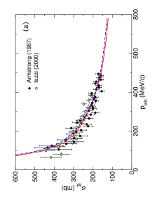
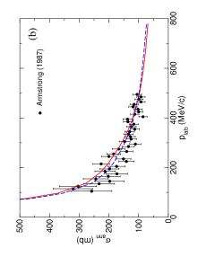
Figure 1: Total (a) and integrated annihilation (b) $\bar{n}p$ cross sections versus beam momentum. The lines show predictions by the Jülich $\bar{N}N$ models A (dashed line) and D (solid line). Data are taken from Refs. Arm87 (circles) and Iaz00 (squares).

Results for the total and integrated elastic ($\bar{p}p$) and charge-exchange ($\bar{p}p\to\bar{n}n$) cross sections and also for angular dependent observables for both models can be found in Refs. Hippchen ; Mull . Evidently, with model A as well as with D a very good overall reproduction of the low- and intermediate energy $\bar{N}N$ data was achieved. Moreover, exclusive data on several $p\bar{p}$ 2-meson and even 3-meson decay channels are described with fair quality Hippchen1 ; Mull ; Betz . Recently, it has been shown that the $N\bar{N}$ models of the Jülich group can also explain successfully the near-threshold enhancement seen in the $\bar{p}p$ mass spectrum of the reactions $J/\Psi\to\gamma\bar{p}p$ Sibi1 , $J/\Psi\to\omega\bar{p}p$ Sibi3 and $B^{+}\to K^{+}\bar{p}p$ Sibi2 and in the $e^{+}e^{-}\to\bar{p}p$ cross section Sibi4 .

As already mentioned in the Introduction, the spin dependence of the $\bar{N}N$ interaction is not well known. There is a fair amount of data on analyzing powers, for $\bar{p}p$ elastic as well as for $\bar{p}p\to\bar{n}n$ charge-exchange scattering, cf. Ref. Klempt for a recent review. However, with regard to other spin-dependent observables there is only scant information on the depolarization $D_{nn}$ and also on $K_{nn}$. Moreover, those data are of rather limited accuracy so that they do not really provide serious constraints on the $\bar{N}N$ interaction. The predictions of the Jülich models A and D are in reasonable agreement with the experimental polarizations up to beam momenta of $p_{lab}\approx 550$ MeV/c as can be seen in Ref. Mull . In fact, model A gives a somewhat better account of the data and reproduces the measured $\bar{p}p$ polarizations even quantitatively up to $p_{lab}\approx 800$ MeV/c ($T_{lab}\approx 300$ MeV). We consider both models here because it allows us to illustrate the influence of uncertainties in the spin-dependence of the $\bar{N}N$ interaction on the spin-dependent cross sections for the $\bar{N}N$ as well as the $\bar{p}d$ systems. In this context let us mention that a partial-wave analysis of $\bar{p}p$ scattering has been performed by the Nijmegen Group Timmermans which, in principle, would allow to pin down the spin-dependence of the $\bar{N}N$ interaction. However, the uniqueness of the achieved solution was disputed in Ref. Richard . Moreover, the actual amplitudes of the Nijmegen analysis are not readily available and, therefore, cannot be utilized for the present investigation.

For the computation of $\bar{p}d$ scattering we also need the $\bar{p}n$ amplitude. For this system, a purely isospin $I=1$ state, there is no experimental information. But there are data for the $\bar{n}p$ channel Arm87 ; Iaz00 , which is identical to the former under the assumption of isospin symmetry. A comparison of our model results with those data is presented in Fig. 1. Obviously the predictions of the Jülich models are in nice agreement with the experimental information on the $\bar{n}p$ interaction too, despite the fact that those total and annihilation cross sections have not been included in the fitting procedure.

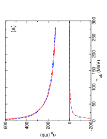
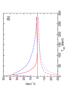
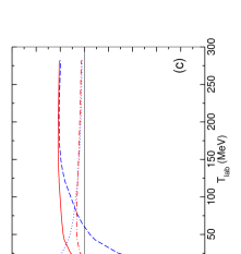
Figure 2: Total $\bar{p}p$ cross sections $\sigma_{0}$ (a), $\sigma_{1}$ (b), and $\sigma_{2}$ (c) versus the antiproton laboratory energy $T_{lab}$. Results based on the purely hadronic amplitude, $\sigma^{h}_{i}$, (model D: solid line, model A: dashed line) and for the Coulomb-nuclear interference term, $\sigma^{int}_{i}$, (D: dash-dotted line, A: dotted line) are shown.

Let us now come to the spin-dependent $\bar{p}p$ and $\bar{p}n$ cross sections predicted by the Jülich $\bar{N}N$ interactions. Corresponding results are presented in Figs. 2 and 3. We display the cross sections based on the purely hadronic amplitude ($\sigma_{i}^{h}$) and the Coulomb-nuclear interference term ($\sigma_{i}^{int}$) separately so that one can see the magnitude of the latter. The total cross sections are then the sum of those two contributions. In the concrete calculations the acceptance angle was chosen to be $\theta_{acc}=8.8$ mrad FILTEX .

At low energies, i.e. around $T_{lab}=5\sim 10$ MeV, the interference terms are comparable to the corresponding purely hadronic cross sections and their magnitude increases further with decreasing energy due to the $1/k_{\bar{p}p}$ factor, cf. Eqs. (IV.1). With increasing energy the relevance of the Coulomb-nuclear interference terms diminishes more and more in case of the cross sections $\sigma_{0}$ and $\sigma_{2}$. But for $\sigma_{1}$ the term is still significant, as one can see from Fig. 2b. The large magnitude of $\sigma_{1}^{int}$ as compared to $\sigma_{1}^{h}$ is due to the fact that $ReM_{2}^{p}(0)\gg ImM_{2}^{p}(0)$ for 100 - 300 MeV, for both $\bar{N}N$ models. As already pointed out in the context of Eqs. (IV.1), $\sigma_{1}^{int}$ is determined by the former quantity but $\sigma_{1}^{h}$ by the latter. Note, that the three cross sections $\sigma_{i}^{int}$ ($i=0,\dots,2$) themselves are all roughly of comparable magnitude for energies from around 50 MeV onwards.

While the predictions of the two models for $\sigma_{0}$ are rather similar (cf. Figs. 2a and 3a), even for the Coulomb-nuclear interference cross section, this is not the case for the spin-dependent cross sections $\sigma_{1}$ and $\sigma_{2}$. For energies below $T_{lab}\approx 150$ MeV there are drastic differences between the results based on the two models. Indeed, for $\sigma_{2}$ at low energies even the sign differs in case of the $\bar{p}p$ channel. Obviously, here the variations in the hadronic amplitude are also reflected in large differences in the Coulomb-nuclear interference term.

For the total $\sigma_{1}$ (including the hadronic and the Coulomb-nuclear interference terms) model A predicts a maximum of 12 mb at the beam energy $T_{lab}\approx 20$ MeV whereas model D yields a maximum of practically the same magnitude at $T_{lab}\approx 10$ MeV. In both cases $\sigma_{1}$ becomes large and negative at very low energies due to the dominance of the Coulomb-nuclear interference term in this region. For comparison, in Ref. DmitrievMS , where a version of the Paris $\bar{N}N$ model was employed, the largest value for $\sigma_{1}$ was found to be -15 mb at $T_{lab}=45$ MeV. In case of $\bar{p}n$ scattering both models exhibit a minimum in $\sigma_{1}$ at $T_{lab}\approx 25$ MeV and reach values of around 20 mb (A) and 50 mb (D) close to threshold.

With regard to $\sigma_{2}$ model A and D predict values around 10 mb for $\bar{p}p$ scattering at higher energies. Close to threshold large negative values are predicted for $\sigma_{2}^{h}+\sigma_{2}^{int}$ due to the Coulomb-nuclear interference term. One should note, however, that for beam energies below 5 MeV, say, the total Coulomb cross section becomes very large. In this case the beam lifetime turns out to be too short and the spin-filtering method cannot be used for polarization buildup in storage ring. The results for $\sigma_{2}$ for $\bar{p}n$ scattering are comparable for both models, reaching a maximum of roughly 30 mb around $T_{lab}=25$ MeV.

Finally, one should note that for both models A and D the polarized cross sections $\sigma_{1}$ and $\sigma_{2}$ exhibit a very different energy dependence in the $\bar{p}p$ and $\bar{p}n$ channels. Thus, the expected polarization buildup for $\bar{p}d$ scattering is likewise different from that of the $\bar{p}p$ reaction, as will be shown in the next section.

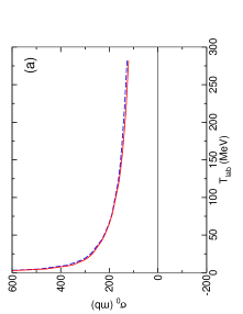
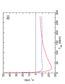
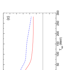
Figure 3: Total $\bar{p}n$ cross sections $\sigma_{0}$ (a), $\sigma_{1}$ (b), and $\sigma_{2}$ (c) versus the antiproton laboratory energy $T_{lab}$. Results for model D (solid line) and model A (dashed line) are shown.

VI Results and discussion of $\bar{p}d$ scattering

In this section we present numerical results for $\bar{p}d$ scattering employing the Jülich models A and D Hippchen ; Mull for the elementary $\bar{p}N$ interactions. In order to estimate the role of the double-scattering mechanism, which will be not taken into account in our calculation of the polarized total cross sections, we first calculate the (unpolarized) total $\bar{p}d$ cross section and also differential cross sections for elastic as well as for elastic plus inelastic scattering events within the Glauber theory. This allows us also to compare our results directly with available $\bar{p}d$ experiments so that we can check the reliability of the approach. As was shown in detail in Refs. Kondratyuksb ; Dalkarov ; mahalabi ; Bendis1 ; Ma ; Bendis2 ; Robson , in forward elastic scattering of antiprotons off nuclei the Glauber theory, though in principle a high-energy approach, works rather well even at fairly low antiproton beam energies like 50 MeV. This has to be compared with proton-nucleus scattering where the Glauber theory is known to give reliable results only for energies in the order of 1 GeV or above. The Glauber theory is applicable at such low energies, because of the presence of annihilation channels in the $\bar{p}N$ interaction. Due to strong annihilation effects, specifically in the $S$-waves, higher partial waves start to play an important role already fairly close to threshold. As a consequence, the $\bar{p}N$ elastic differential cross section is peaked in forward direction already at rather low energies Mull ; Klempt and, therefore, suitable for application of the eikonal approximation, which is the basis of the Glauber theory. In other words it can be seen from the optical theorem that the higher the annihilation cross section is, the larger is the modulus of the forward elastic scattering amplitude. Indeed, the elastic spin-averaged $\bar{p}N$ scattering amplitude can be very well parameterized by

$$f_{\bar{p}N}(q)=\frac{k_{\bar{p}N}\sigma^{\bar{p}N}_{tot}(i+\alpha_{\bar{p}N})}{4\pi}\exp{(-\beta^{2}_{\bar{p}N}q^{2}/2)},$$ (28)

where $\sigma^{\bar{p}N}_{tot}$ is the total unpolarized $\bar{p}N$ cross section, $\alpha_{\bar{p}N}$ is the ratio of the real to imaginary part of the forward scattering amplitude $f_{\bar{p}N}(0)$, $\beta_{\bar{p}N}^{2}$ is the slope of the diffraction cone, $q$ is the transferred 3-momentum, and $k_{\bar{p}N}$ is the $\bar{p}N$ cms momentum.

Table 1: Parameters of the $\bar{p}p$ and $\bar{p}n$ amplitudes according to Eq. (28) representing the results of the $\bar{N}N$ models A and D of the Jülich group Mull at different beam energies. Note that the values for $\sigma_{tot}^{\bar{p}N}$ and $\alpha_{\bar{p}N}$ follow directly from the corresponding models, while $\beta_{\bar{p}N}^{2}$ is determined in a fit to the corresponding amplitudes.

$T_{lab}$	$\bar{p}N$ model	$\sigma_{tot}^{\bar{p}p}$	$\beta_{\bar{p}p}^{2}$	$\alpha_{\bar{p}p}$	$\sigma_{tot}^{\bar{p}n}$	$\beta_{\bar{p}n}^{2}$	$\alpha_{\bar{p}n}$
MeV		mb	(GeV/c)-2		mb	(GeV/c)-2
10	A	409	46.24	-0.351	372	41.1	-0.372
	D	441	59.1	-0.20	354.	51.4	-0.164
25.5	A	305	46.24	-0.176	267.2	36.0	-0.146
	D	312	52.4	-0.130	260	48.8	-0.076
50	A	233.5	33	-0.095	209.6	26	-0.034
	D	240	33.47	-0.121	219	33.47	-0.058
78	A	209.5	29.9	-0.03	192.6	26	0.0417
	D	203	29.9	-0.03	192	29.2	0.0145
109	A	186	25.2	0.033	171.3	24	0.108
	D	175.8	25.9	-0.029	165	25	0.0245
124	A	174.4	24.45	0.057	163.	24.3	0.133
	D	168.4	24.45	-0.030	159.5	24.3	0.0245
138	A	174.0	23.24	-0.030	159.5	22.9	-0.03
	D	162.5	23.24	-0.030	155	22.9	-0.03
149	A	164	22.58	0.009	156.2	22.58	0.166
	D	159.26	22.58	0.002	149	22.58	0.056
179	A	156.3	23.4	0.110	148	20.7	0.187
	D	150.	23.4	-0.0256	143	20.7	-0.0816

Figure 4: Differential cross section of $\bar{p}p$ (left panel) and $\bar{p}n$ (right panel) elastic scattering predicted by model A versus the c.m.s. scattering angle $\Theta$ at different beam energies: 50 MeV (dashed-dotted line), 25 MeV (dotted), 10 MeV (solid).

For the present investigation we utilize Eq. (28) to represent the scattering amplitudes of the Jülich models in analytical form. This allows us then to evaluate the $\bar{p}d$ scattering amplitude as given in Eq. (11) in a straight-forward way, including also the double-scattering correction. The values for the parameters $\sigma^{\bar{p}N}_{tot}$ and $\alpha_{\bar{p}N}$ can be taken directly from the $\bar{p}N$ scattering amplitudes $M_{i}^{N}(0)$ that result from the considered Jülich models. The parameters $\beta^{2}_{\bar{p}N}$ are determined in a fit of $|f_{\bar{p}N}(q)|^{2}$ to the unpolarized differential cross section $d\sigma/d\Omega(\theta)$ resulting from the employed $\bar{N}N$ models. We found that even at beam energies as low as 10-25 MeV the parameter $\beta^{2}_{\bar{p}N}$ is large, i.e. $40-50$ (GeV/c)², reflecting the fact that the elastic amplitude in Eq. (28) is indeed peaked in forward direction. For illustration purposes we present $\bar{p}p$ and $\bar{p}n$ differential cross sections at three selected energies in Fig. 4 for model A. The concrete parameters for the $\bar{p}p$ and $\bar{p}n$ amplitudes at the various energies are summarized in Table 1.

Table 2: Total unpolarized $\bar{p}d$ cross sections calculated within the Glauber theory in the impulse approximation ($\sigma^{IA}_{tot}$) and with $\bar{p}N$ double scattering included ($\sigma_{tot}$). The $\bar{N}N$ model D of the Jülich group Mull is used. Experimental values ($\sigma^{exp}_{tot}$) at the various beam energies $T_{lab}$ are taken from Refs. Kalogeropoulos (a), Burrows (b) and BizzarriNC74 (c).

$T_{lab}$	$\sigma^{exp}_{tot}$	$\sigma_{tot}$	$\sigma^{IA}_{tot}$	$R=\sigma^{IA}_{tot}/\sigma_{tot}$
MeV	mb	mb	mb
57.0	415$\pm 16^{a)}$	401	471	1.17
58.0	390$\pm 15^{b)}$	401	471	1.17
57.4$\pm 13.2$	366.2$\pm 11.5^{c)}$
79.8$\pm 10.0$	346.4$\pm 8.4^{c)}$	339	395	1.16
109.3	322 $\pm 16^{a)}$	296	341	1.15
109.3$\pm 8.8$	310.7$\pm 7.3^{c)}$
124.1$\pm 8.1$	287.5$\pm 6.1^{c)}$	286	328	1.15
126.8	295$\pm 7^{b)}$
137.7 $\pm 7.5$	283.4$\pm 5.4^{c)}$	277	317	1.15
147	271$\pm 6^{b)}$	270	308	1.14
146.6$\pm 7.1$	282.6$\pm 5.4^{c)}$
179.3	269$\pm 7^{b)}$	258	293	1.14
170.5$\pm 8.8$	271.8$\pm 4.2^{c)}$	264	301	1.14

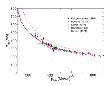
Figure 5: Total $\bar{p}d$ cross section versus the beam momentum $p_{lab}$. The solid and dashed lines are results based on the $\bar{N}N$ models D and A, respectively. The dotted line is the results for model D obtained within the single-scattering approximation. Data are taken from Refs. BizzarriNC74 ; Kalogeropoulos ; Burrows ; Carroll ; Hamilton .

Figure 6: Elastic (lower lines) and elastic plus inelastic (upper lines) $\bar{p}d$ differential cross sections versus the transferred momentum for different $\bar{p}$ beam energies. The lines are results of a calculation based on the Glauber theory for model A (dotted and dashed-dotted) and D (solid and dashed) utilizing the parameterizations of the $\bar{p}N$ amplitudes given in Table 1. The ABB form factor ABB is used for the deuteron. Data for elastic scattering (179.3 MeV) are taken from bruge88 (squares) and for elastic plus inelastic scattering events (57.4 - 170.5 MeV) from BizzarriNC74 (circles).

Results for the total unpolarized $\bar{p}d$ cross section are displayed in Fig. 5 together with experimental information BizzarriNC74 ; Kalogeropoulos ; Burrows ; Carroll ; Hamilton . A comparision of theory with data at selected energies is presented in Table 2 for model D. One can see that the single-scattering approximation (shown here only for model D) overestimates the total unpolarized cross section by roughly 15%, cf. the dotted line in Fig. 5. But the shadowing effect generated by the $\bar{p}N$ double-scattering mechanism reduces the cross section by about that amount so that the final result (solid line) is in good agreement with the experiment. The results for model A are very similar. Thus, as expected the double-scattering corrections to the total unpolarized cross section turn out to be not very large. Actually, even at energies as low as 10 - 20 MeV they are at most 20-25%. Therefore, the Glauber theory seems to work rather well for the $\bar{p}d$ reaction, even at these fairly low energies.

Predictions for differential cross sections are presented in Fig. 6. In the corresponding calculations of the forward $\bar{p}d$ elastic amplitude the single-scattering mechanism as well as the double-scattering terms were included. The ABB form factor ABB is used for the deuteron. At $T_{lab}$ = 179.3 MeV data for the elastic differential cross section are available bruge88 . These data (squares in Fig. 6) are nicely reproduced by our model calculation for forward angles. Also the differential cross sections for elastic (${\bar{p}}d\to{\bar{p}}d$) plus inelastic (${\bar{p}}d\to{\bar{p}}pn$) scattering events, measured at the neighboring energy $T_{lab}$ = 170 MeV BizzarriNC74 (circles), are well described. At lower energies no data on the elastic differential cross section are available. But there are further angular distributions published in Ref. BizzarriNC74 . In Fig. 6 we show results for selected energies, namely 57.4 MeV, 78 MeV, and 138 MeV. Obviously, our model results are in line with those data down to the lowest energy.

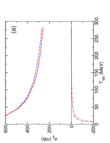
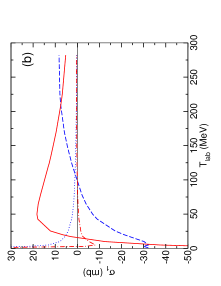
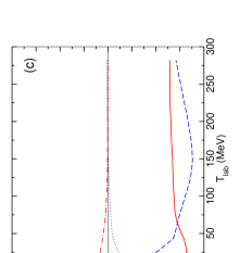
Figure 7: Total $\bar{p}d$ cross sections $\sigma_{0}$ (a), $\sigma_{1}$ (b), and $\sigma_{2}$ (c) versus the antiproton laboratory energy $T_{lab}$. Results based on the purely hadronic amplitude, $\sigma^{h}_{i}$, (model D: solid line, model A: dashed line) and for the Coulomb-nuclear interference term, $\sigma^{int}_{i}$, (D: dash-dotted line, A: dotted line) are shown.

Results for spin-dependent cross sections are presented in Fig. 7. Note that here the corresponding calculations are all done in the single-scattering approximation only. In principle, the double-scattering corrections to the spin-dependent cross sections could be worked out by adopting the formalism described in Refs. Alberi ; Alberi1 ; Sorensen . But we expect that the double-scattering effects on those quantities are roughly of the same magnitude (i.e. less than 20 % for energies above 20 MeV) as for the spin-independent cross sections. At least this is what we find numerically within the approximation outlined in Ref. Alberi . Therefore, we believe that the single-scattering approximation provides a reasonable estimation for the magnitude of the polarization buildup effect in $\bar{p}d$ scattering and we refrain from a thorough evaluation of the involved double-scattering effects in the present analysis. After all one has to keep in mind that the differences between the $\bar{N}N$ models A and D introduce significantly larger variations in the cross sections $\sigma_{1}$ and $\sigma_{2}$, cf. Fig. 7b and c.

Figure 8: Ratio of the total polarized cross sections to the total unpolarized cross section, $\sigma_{1}/\sigma_{0}$ (a) and $\sigma_{2}/\sigma_{0}$ (b), versus beam energy. Results for $\bar{p}d$ scattering [model A (dashed line), D (solid line)] as well as for $\bar{p}p$ scattering [model A (dashed-dotted), D (dotted)] are displayed. The Coulomb-nuclear interference cross sections $\sigma_{i}^{int}$ $(i=0,1,2)$ for $\theta_{acc}=8$ mrad are included.

The $\bar{N}N$ model D predicts large spin-dependent cross section $\sigma_{1}$ with a maximum around 40 MeV. The cross section $\sigma_{2}$ is large as well and practically constant from around 75 MeV onwards. In case of model A the maximum for $\sigma_{1}$ occurs at considerably higher energies. Large negative values of $\sigma_{1}$ are predicted for energies below 50 MeV with a maximum at 150 MeV. The predictions for $\sigma_{2}$ are comparable to those of model D for energies above 25 MeV, say. As one can see from Fig. 7, the largest values for the polarized $\bar{p}d$ cross sections are expected at very low energies, i.e. for $T_{lab}$ less than 10 MeV, since the $\bar{p}N$ cross sections increase with decreasing beam energy. However, as was already noted above, at these energies the pure Coulomb cross section becomes too large, so that the method of spin-filtering for the polarization buildup cannot be applied due to the decrease of the beam lifetime. In any case, while our results at higher energies are expected to be correct within 10% to 20 %, there are larger uncertainties below 20 MeV and here our results should be considered only as a qualitative estimate. Finally, one can see from Fig. 7, that the Coulomb-nuclear interference effects become only important for energies below 50 MeV. In contrast to the $\bar{p}p$ case, for $\bar{p}d$ $\sigma_{1}^{int}$ is much smaller than $\sigma_{1}^{h}$ at $T_{lab}\geq 100$ MeV. This different behavior for $\bar{p}p$ and $\bar{p}d$ is due to the additional terms $M_{i}^{n}(0)$ entering the expression for $\sigma_{i}^{int}$ of the latter reaction, as explained in Sect. IV.2.

The polarization buildup is determined mainly by the ratio of the polarized total cross section $\sigma_{i}$ (i=1,2) to the unpolarized one ($\sigma_{0}$). Those ratios $\sigma_{i}/\sigma_{0}$ are shown in Fig. 8 for beam energies 10-300 MeV for the $\bar{p}p$ and $\bar{p}d$ reactions. The Coulomb-nuclear interference effects are taken into account. Once again those results exhibit a significant model dependence. However, for all considered cases large values for the ratio $\sigma_{2}/\sigma_{0}$ of around 10% are predicted at the higher energies, which would be sufficient for the requirements of the PAX experiment Frankpc . Also, when comparing the $\bar{p}p$ and $\bar{p}d$ results we see that (the moduli of) the predicted values for the ratio $\sigma_{2}/\sigma_{0}$ are larger for $\bar{p}d$ than for $\bar{p}p$, for energies of $T_{lab}\approx$ 100 MeV or higher, in case of model A as well as for model D. Thus, our results suggest that there could be indeed a slightly higher efficiency for the polarization buildup when using $\bar{p}d$ instead of $\bar{p}p$.

VII Summary

In the present paper we employed two $\bar{N}N$ potential models developed by the Jülich group for a calculation of unpolarized $\bar{p}d$ scattering within the Glauber-Sitenko theory and found that this approach allows one to describe the experimental information on differential and total $\bar{p}d$ cross sections, available at $T_{lab}=50-180$ MeV, quantitatively. For those spin-independent observables the difference in the predictions based on those two models turned out to be rather small. The double-scattering corrections to the unpolarized cross section were found to be in the order of 15% in the energy range where the data are available. But we found that even at such low energies as 10-25 MeV they are not larger than 20-25%. This means that, most likely, the Glauber approximation does work reasonably well for $\bar{p}d$ scattering down to fairly small energies.

We also presented results for polarized $\bar{p}d$ cross sections obtained within the single-scattering approximation. In comparison to $\bar{p}p$ scattering, for $\bar{p}d$ scattering there are four total polarized cross sections instead of the three in the $\bar{p}p$ case. The additional cross section, connected with the tensor polarization $P_{zz}^{d}$ of the deuteron, has no direct influence on the polarization buildup, but, in principle, can be used to increase the beam lifetime by a proper choice of the sign of $P_{zz}^{d}$.

In the single-scattering approximation the spin dependent $\bar{p}d$ cross sections are given by the sum of the corresponding $\bar{p}p$ and $\bar{p}n$ cross sections. As a consequence, at some energies there is an increase of the polarized cross sections as compared to the $\bar{p}p$ and/or $\bar{p}n$ case. The Coulomb-nuclear interference effects in the polarized cross sections, which play an important role for the $pp$ and $\bar{p}p$ systems, are modified in $\bar{p}d$ scattering due to the additional interference with the purely hadronic $\bar{p}n$ amplitude.

The predictions for the spin-dependent cross sections for $\bar{p}d$ scattering, presented in this work, exhibit a fairly strong model dependence, which is due to uncertainties in the spin dependence of the elementary $\bar{p}p$ and $\bar{p}n$ interactions. Still, our results suggest that $\bar{p}d$ elastic scattering can be used for the polarization buildup of antiprotons at beam energies of 10-300 MeV with similar and possibly even higher efficiency than $\bar{p}p$ scattering.

Acknowledgements

We acknowledge stimulating discussions with N.N. Nikolaev and F. Rathmann. Furthermore, we are thankful to A.I. Milstein, V.M. Strakhovenko and H. Ströher for reading the manuscript and useful remarks. This work was supported in part by the Heisenberg-Landau program.

Appendix: Coulomb-nuclear interference cross sections for $\bar{p}d$ elastic scattering

In the coordinate system with the axes $OX||{\bf l}$, $OY||{\bf n}$, $OZ||{\bf m}$, where

$${\bf l}=({\bf k}+{\bf k}^{\prime})/|{\bf k}+{\bf k}^{\prime}|,\ {\bf m}=({\bf k}-{\bf k}^{\prime})/|{\bf k}-{\bf k}^{\prime}|,\ {\bf n}=[{\bf k}\times{\bf k}^{\prime}]/|[{\bf k}\times{\bf k}^{\prime}]|,$$ (A.1)

one can find for the operators ${\hat{F}}_{\alpha\beta}$ defined by Eq. (3) the following structure KLEVSH

$${\hat{F}}_{xx} = \phantom{-}F_{1}+F_{2}{\hat{\sigma}_{y}},\ \ {\hat{F}}_{xy}=\phantom{-}F_{7}{\hat{\sigma}_{z}}+F_{8}{\hat{\sigma}_{x}},\ \ {\hat{F}}_{xz}=\phantom{-}F_{9}+F_{10}{\hat{\sigma}_{y}},$$

$${\hat{F}}_{yx} = -F_{7}{\hat{\sigma}_{z}}+F_{8}{\hat{\sigma}_{y}},\ \ {\hat{F}}_{yy}=F_{3}+F_{4}{\hat{\sigma}_{y}},\ \ {\hat{F}}_{yz}=F_{11}{\hat{\sigma}_{x}}+F_{12}{\hat{\sigma}_{z}},$$

$${\hat{F}}_{zx} = -F_{9}-F_{10}{\hat{\sigma}_{y}},\ \ {\hat{F}}_{zy}=-F_{11}{\hat{\sigma}_{x}}+F_{12}{\hat{\sigma}_{z}},\ \ {\hat{F}}_{zz}=F_{5}+F_{6}{\hat{\sigma}_{y}},$$ (A.2)

where the $F_{i}$’s are complex numbers and $\hat{\sigma}_{j}$ $(j=x,y,z)$ are the Pauli matrices. Using Eqs. (Appendix: Coulomb-nuclear interference cross sections for $\bar{p}d$ elastic scattering) the spin correlation parameters can be written in the following form:

$$C_{x,x} = \frac{2}{B}\Bigl{\{}Im(F_{9}F_{8}^{*}+F_{11}F_{3}^{*}+F_{11}F_{5}^{*})+Re(F_{7}F_{10}^{*}-F_{4}F_{12}^{*}+F_{12}F_{6}^{*})\Bigr{\}},$$

$$C_{y,y} = \frac{2}{B}\Bigl{\{}Im(F_{1}F_{10}^{*}+F_{2}F_{9}^{*}+F_{6}F_{9}^{*}+F_{5}F_{10}^{*})-Re(F_{11}F_{7}^{*}+F_{12}F_{8}^{*})\Bigr{\}},$$

$$C_{z,z} = \frac{2}{B}\Bigl{\{}Im(F_{7}F_{1}^{*}+F_{7}F_{3}^{*}+F_{9}F_{12}^{*})+Re(F_{2}F_{8}^{*}-F_{8}F_{4}^{*}+F_{10}F_{11}^{*})\Bigr{\}},$$

$$C_{x,z} = \frac{2}{B}\Bigl{\{}Im(F_{1}F_{8}^{*}+F_{8}F_{3}^{*}+F_{9}F_{11}^{*})+Re(F_{2}F_{7}^{*}+F_{7}F_{4}^{*}-F_{10}F_{12}^{*})\Bigr{\}},$$

$$C_{z,x} = \frac{2}{B}\Bigl{\{}Im(F_{7}F_{9}^{*}+F_{3}F_{12}^{*}+F_{12}F_{5}^{*})+Re(F_{8}F_{10}^{*}-F_{4}F_{11}^{*}-F_{11}F_{6}^{*})\Bigr{\}},$$ (A.3)

where $B$ is given by

$$B=\sum_{i=1}^{6}|F_{i}|^{2}+2\sum_{i=7}^{12}|F_{i}|^{2}.$$

The tensor analyzing powers $A_{ij}$ can be expressed in the following form (see, for example, KLEVSH ):

$$A_{xx} = \frac{1}{B}\Bigl{\{}|F_{3}|^{2}+|F_{4}|^{2}+|F_{5}|^{2}+|F_{6}|^{2}-(|F_{7}|^{2}+|F_{8}|^{2}$$

$$+|F_{9}|^{2}+|F_{10}|^{2})-2(|F_{1}|^{2}+|F_{2}|^{2}-|F_{11}|^{2}-|F_{12}|^{2})\Bigr{\}},$$

$$A_{yy} = \frac{1}{B}\Bigl{\{}|F_{1}|^{2}+|F_{2}|^{2}+|F_{5}|^{2}+|F_{6}|^{2}-(|F_{7}|^{2}+|F_{8}|^{2}$$

$$+|F_{11}|^{2}+|F_{12}|^{2})-2(|F_{3}|^{2}+|F_{4}|^{2}-|F_{9}|^{2}-|F_{10}|^{2}\Bigr{\}},$$

$$A_{zz} = -A_{xx}-A_{yy},$$

$$A_{xz} = -\frac{3}{B}Re\Bigl{[}F_{7}F_{12}^{*}+F_{9}F_{5}^{*}+F_{10}F_{6}^{*}-F_{2}F_{10}^{*}-F_{1}F_{9}^{*}-F_{8}F_{11}^{*}\Bigr{]}.$$ (A.4)

The polarized elastic differential $\bar{p}d$ cross section is

$$\Bigl{(}\frac{d\sigma}{d\Omega}\Bigr{)}_{pol}=\Bigl{(}\frac{d\sigma}{d\Omega}\Bigr{)}_{0}\Bigl{[}1+\frac{3}{2}p_{j}^{\bar{p}}p_{i}^{d}C_{j,i}+\frac{1}{3}P_{ij}^{d}A_{ij}+\dots\Bigr{]}.$$ (A.5)

Here $\Bigl{(}\frac{d\sigma}{d\Omega}\Bigr{)}_{0}$ is the unpolarized differential cross section, which is given as

$$\Bigr{(}\frac{d\sigma}{d\Omega}\Bigr{)}_{0}=\frac{1}{3}\Bigl{[}\sum_{i=1}^{6}|F_{i}|^{2}+2\sum_{i=7}^{12}|F_{i}|^{2}\Bigr{]}=\frac{1}{3}B.$$ (A.6)

In Eq. (A.5) we spell out explicitly only those terms which give a non-zero contribution to the total elastic polarized cross section, while other occuring terms are denoted by dots. The total elastic polarized cross section can be found by integration of Eq. (A.5) over the scattering angle:

$$\sigma_{pol}^{el}=2\pi\int_{\theta_{acc}}^{\pi}\Bigl{(}\frac{d\sigma}{d\Omega}\Bigr{)}_{pol}\sin{\theta}d\theta.$$ (A.7)

The Coulomb amplitudes are contained only in the following terms: $F_{1}=F_{1}^{h}+F_{1}^{C}$, $F_{3}=F_{3}^{h}+F_{3}^{C}$, and $F_{5}=F_{5}^{h}+F_{5}^{C}$, where $F_{i}^{h}$ is the purely hadronic part of the amplitudes in question. Due to the singularity $\sim\sin^{-2}({\theta/2})$ of the Coulomb amplitudes $F_{1}^{C}=F_{3}^{C}=F_{5}^{C}\equiv F^{C}$ the main contribution to the Coulomb-nuclear interference terms in the cross section Eq. (A.5) comes from forward angles and, therefore, is non-vanishing only for those hadronic amplitudes $F_{i}$ which are non-zero in forward direction. In the limit of collinear kinematics when $OZ||{\bf k}||{\bf k}^{\prime}$ ($\theta=0^{o}$), one can find from Eqs. (2) and (Appendix: Coulomb-nuclear interference cross sections for $\bar{p}d$ elastic scattering) uzepan98

$$F_{1}^{h}=F_{3}^{h}=g_{1},\ \ F_{5}^{h}=g_{2},\ \ F_{7}^{h}=ig_{4},\ \ F_{10}^{h}=-F_{11}^{h}=-ig_{3},$$

$$F_{2}^{h}=F_{4}^{h}=F_{6}^{h}=F_{8}^{h}=F_{9}^{h}=F_{12}^{h}=0.$$ (A.8)

Based on these relations one obtains via Eqs. (Appendix: Coulomb-nuclear interference cross sections for $\bar{p}d$ elastic scattering), (Appendix: Coulomb-nuclear interference cross sections for $\bar{p}d$ elastic scattering):

$$C_{z,z}(0)=\frac{2}{B}\bigl{\{}ImF_{7}(F_{1}^{*}+F_{3}^{*})+ReF_{10}F_{11}^{*}\bigl{\}},$$

$$C_{x,x}(0)=C_{y,y}(0)=\frac{2}{B}Im(F_{1}+F_{5})F_{10}^{*},$$

$$A_{xx}(0)=A_{yy}(0)=-\frac{1}{2}A_{zz}(0)=\frac{1}{B}\bigl{\{}-|F_{1}|^{2}+|F_{5}|^{2}+|F_{11}|^{2}-|F_{7}|^{2}\bigl{\}},$$

$$C_{z,x}(0)=C_{x,z}(0)=A_{xz}(0)=0.$$ (A.9)

Taking into account axial symmetry, which follows from Eqs. (Appendix: Coulomb-nuclear interference cross sections for $\bar{p}d$ elastic scattering), the polarized Coulomb-nuclear interference cross section can be written as

$$\sigma_{pol}^{int}=2\pi\int_{\theta_{acc}}^{\pi}\Bigl{(}\frac{d\sigma}{d\Omega}\Bigr{)}_{pol}\Bigl{\{}1+\frac{3}{2}C_{x,x}{\bf P}^{\bar{p}}{\bf P}^{d}+\frac{3}{2}(C_{z,z}-C_{x,x})P_{z}^{\bar{p}}{P_{z}}^{d}+\frac{1}{3}(A_{xx}-A_{zz})P_{zz}^{d}\Bigr{\}}\sin{\theta}d\theta.$$ (A.10)

Using Eqs. (Appendix: Coulomb-nuclear interference cross sections for $\bar{p}d$ elastic scattering)-(Appendix: Coulomb-nuclear interference cross sections for $\bar{p}d$ elastic scattering) and performing the integration over the scattering angle in Eq. (A.10), one can find finally

$$\sigma_{0}^{int} = \frac{4\pi}{3}\int_{\theta_{acc}}^{\pi}Re\Bigl{\{}[{F_{1}^{h}}^{*}(0)+{F_{3}^{h}}^{*}(0)+{F_{5}^{h}}^{*}(0)]F_{1}^{C}\Bigr{\}}\sin{\theta}d\theta,$$

$$\sigma_{1}^{int} = 2\pi\int_{\theta_{acc}}^{\pi}Im\bigl{\{}{F_{10}^{h}}^{*}(0)(F_{3}^{C}+F_{5}^{C})\Bigr{\}}\sin{\theta}d\theta,$$

$$\sigma_{2}^{int} = -2\pi\int_{\theta_{acc}}^{\pi}Im\Bigl{\{}[{F_{7}^{h}}^{*}(0)+{F_{10}^{h}}^{*}(0)](F_{1}^{C}+F_{3}^{C})\Bigr{\}}\sin{\theta}d\theta,$$

$$\sigma_{3}^{int} = \frac{4\pi}{3}\int_{\theta_{acc}}^{\pi}Re\Bigl{\{}[{F_{3}^{h}}^{*}(0)-{F_{5}^{h}}^{*}(0)]F_{1}^{C}\Bigr{\}}\sin{\theta}d\theta.$$ (A.11)

References

- (1) V. Barone et al. [PAX Collaboration], arXiv:hep-ex/0505054.
- (2) F. Rathmann et al., Phys. Rev. Lett. 94, 014801 (2005) [arXiv:physics/0410067].
- (3) F. Rathmann et al., Phys. Rev. Lett. 71, 1379 (1993).
- (4) A.I. Milstein and V.M. Strakhovenko, Phys. Rev. E 72, 066503 (2005).
- (5) N.N. Nikolaev and F. Pavlov, arXiv:hep-ph/0512051.
- (6) N.N. Nikolaev and F. Pavlov, AIP Conf. Proc. 915, 932 (2007) [arXiv:hep-ph/0701175].
- (7) N.N. Nikolaev and F. Pavlov, AIP Conf. Proc. 1008, 34 (2008).
- (8) H.O. Meyer, Phys. Rev. E 50, 1485 (1994).
- (9) P. Lenisa and F. Rathmann [PAX Collaboration], arXiv:nucl-ex/0512021.
- (10) V. F. Dmitriev, A. I. Milstein and V. M. Strakhovenko, Nucl. Instrum. Meth. B 266, 1122 (2008) [arXiv:0707.3006 [hep-ph]].
- (11) T. Hippchen, J. Haidenbauer, K. Holinde and V. Mull, Phys. Rev. C 44, 1323 (1991).
- (12) V. Mull, J. Haidenbauer, T. Hippchen and K. Holinde, Phys. Rev. C 44, 1337 (1991).
- (13) V. Mull and K. Holinde, Phys. Rev. C 51, 2360 (1995).
- (14) H. Arenhövel, arXiv:0706.3576 [nucl-th].
- (15) T. Walcher, H. Arenhövel, K. Aulenbacher, R. Barday and A. Jankowiak, Eur. Phys. J. A 34, 447 (2007) [arXiv:0706.3765 [physics.acc-ph]].
- (16) A. I. Milstein, S. G. Salnikov and V. M. Strakhovenko, Nucl. Instrum. Meth. B 266, 3453 (2008) [arXiv:0802.3766 [hep-ph]].
- (17) F. Rathmann, private communication.
- (18) V.A. Chetvertkova and S.B. Nurushev, talk at the XIX Baldin ISHEPP Seminar, Dubna, 29 September - 4 October, 2008.
- (19) R.J.N. Phillips, Nucl. Phys. 43, 413 (1963).
- (20) M.P. Rekalo, N.M. Piskunov and I.M. Sitnik, Few-Body Syst. 23, 187 (1998).
- (21) Yu.N. Uzikov, Phys. Elem. Chast. At. Yadr. 29, 1405 (1998) [Phys. Part. Nucl. 29, 583 (1998)].
- (22) V. Franco and R.J. Glauber, Phys. Rev. 142, 1195 (1966).
- (23) J. Mahalanabis, Z. Phys. A 342, 101 (1992).
- (24) J. Bystricky, F. Lehar and P. Winternitz, J. Phys. (France) 39, 1 (1978).
- (25) G. Alberi, M. Bleszynski, T. Jaroszewicz and S. Santos, Phys. Rev. D 20, 2437 (1979).
- (26) G. Alberi, M. Bleszynski and T. Jaroszewicz, Ann. Phys. 142, 299 (1982).
- (27) L.D. Landau and E.M. Lifschitz, Quantum Mechanics, Nonrelativistic Theory (Pergamon, Oxford, 1965).
- (28) H. Lesniak and L. Lesniak, Nucl. Phys. B 38, 221 (1972).
- (29) R. Machleidt, K. Holinde and Ch. Elster, Phys. Rep. 149, 1 (1987).
- (30) M. Betz, E. A. Veit and J. Haidenbauer, Eur. Phys. J. A 14, 113 (2002) [arXiv:nucl-th/0203068].
- (31) A. Sibirtsev, J. Haidenbauer, S. Krewald, U. G. Meißner and A. W. Thomas, Phys. Rev. D 71, 054010 (2005) [arXiv:hep-ph/0411386].
- (32) J. Haidenbauer, U. G. Meißner and A. Sibirtsev, Phys. Lett. B 666, 352 (2008) [arXiv:0804.1469 [hep-ph]].
- (33) J. Haidenbauer, U. G. Meißner and A. Sibirtsev, Phys. Rev. D 74, 017501 (2006) [arXiv:hep-ph/0605127].
- (34) J. Haidenbauer, H. W. Hammer, U. G. Meißner and A. Sibirtsev, Phys. Lett. B 643, 29 (2006) [arXiv:hep-ph/0606064].
- (35) E. Klempt, F. Bradamante, A. Martin and J. M. Richard, Phys. Rept. 368, 119 (2002).
- (36) R. Timmermans, T. A. Rijken and J. J. de Swart, Phys. Rev. C 50, 48 (1994) [arXiv:nucl-th/9403011].
- (37) J. M. Richard, Phys. Rev. C 52, 1143 (1995).
- (38) T. Armstrong et al., Phys. Rev. D 36, 659 (1987).
- (39) F. Iazzi et al., Phys. Lett. B 475, 378 (2000).
- (40) L.A. Kondratyuk, M.Zh. Shmatikov and R. Bizzarri, Yad. Fiz. 33, 795 (1981) [Sov. J. Nucl. Phys. 33, 413 (1981)].
- (41) O.D. Dalkarov and V.A. Karmanov, Phys. Lett. 147B, 1 (1984); Nucl. Phys. A 445, 579 (1985).
- (42) G. Bendiscioli, A. Rotondi, P. Salvini and A. Zenoni, Nucl. Phys. A 469, 669 (1987).
- (43) W. H. Ma and D. Strottman, Phys. Rev. C 44, 615 (1991).
- (44) G. Bendiscioli, A. Rotondi and A. Zenoni, Nuovo Cim. A 105, 1055 (1992).
- (45) Y. S. Zhang and B. A. Robson, Eur. Phys. J. A 22, 515 (2004).
- (46) R. Bizzarri et al., Nuovo Cim. 22 A, 225 (1974).
- (47) T. Kalogeropoulos and G.S. Tzankos, Phys. Rev. D 22, 2585 (1980).
- (48) R.D. Burrows et al., Austr. J. Phys. 23, 819 (1970).
- (49) A.S. Carroll et al., Phys. Rev. Lett. 32, 247 (1974).
- (50) R.P. Hamilton et al., Phys. Rev. Lett. 44, 1182 (1980).
- (51) B.S. Aladashvili et al., J. Phys. G 3, 7 (1977).
- (52) G. Bruge et al., Phys. Rev. C 37 , 1345 (1988).
- (53) C. Sorensen, Phys. Rev. D 19, 1444 (1979).
- (54) L.A. Kondratyuk, F.M. Lev and L.V. Schevchenko, Yad. Fiz. 33, 1208 (1981) [Sov. J. Nucl. Phys. 33 , 642 (1982)].