Statistics of spikes trains, synaptic plasticity and Gibbs distributions.

Abstract

We introduce a mathematical framework where the statistics of spikes trains, produced by neural networks evolving under synaptic plasticity, can be analysed.

1 Introduction.

Synaptic plasticity occurs at many levels of organization and time scales in the nervous system [1]. It is of course involved in memory and learning mechanisms, but it also alters excitability of brain area and regulates behavioural states (e.g. transition between sleep and wakeful activity). Therefore, understanding the effects of synaptic plasticity on neurons dynamics is a crucial challenge. However, the exact relation between the synaptic properties (“microscopic” level) and the effects induced on neurons dynamics (meso-or macroscopic level) is still highly controversial.

On experimental grounds, synaptic changes can be induced by specific simulations conditions defined through the firing frequency of pre- and postsynaptic neurons [2, 3], the membrane potential of the postsynaptic neuron [4], spike timing [5, 6, 7] (see [8] for a review). Different mechanisms have been exhibited from the Hebbian’s ones [9] to Long Term Potentiation (LTP) and Long Term Depression (LTD), and more recently to Spike Time Dependent Plasticity (STDP) [6, 7] (see [10, 11, 12] for a review). Most often, these simulation are performed in isolated neurons in in vitro conditions. Extrapolating the action of these mechanisms to in vivo neural networks requires both a bottom-up and up-bottom approach.

This issue is tackled, on theoretical grounds, by infering “synaptic updates rules” or “learning rules” from biological observations [13, 1, 14] (see [10, 11, 12] for a review) and extrapolating, by theoretical or numerical investigations, what are the effects of such synaptic rule on such neural network model. This approach relies on the belief that there are “canonical neural models” and “canonical plasticity rules” capturing the most essential features of biology. Unfortunately, this results in a plethora of canonical “candidates” and a huge number of papers and controversies. Especially, STDP deserved a long discussion either on its biological interpretation or on its practical implementation [15]. Also, the discussion of what is relevant for neuron coding and what has to be measured to conclude on the effects of synaptic plasticity is a matter of long debates (rate coding, rank coding, spike coding ?) [16, 17]

In an attempt to clarify and unify the overall vision, some researchers have proposed to associate learning rules and their dynamical effects to general principles, and especially to“variational” or “optimality” principles, where some functional has to maximised or minimised (known examples of variational principles in physics are least-action or entropy maximization). Dayan and Hausser [18] have shown that STPD can be viewed as an optimal noise-removal filter for certain noise distributions, Rao and Sejnowski [19, 20] suggested that STDP may be related to optimal prediction (a neuron attemps to predict its membrane potential at some time, given the past). Bohte and Mozer [21] proposes that STPD minimizes response variability. Chechik [22] relates STDP to information theory via maximisation of mutual information between input and output spike trains. In the same spirit, Toyoizumi et al [23, 24] have proposed to associate STDP to an optimality principle where transmission of information between an ensemble of presynaptic spike trains and the ouput spike train of the postsynaptic neuron is optimal, given some constraints imposed by biology (such as homeostasy and minimisation in the number of strong synapses, which is costly in view of continued protein synthesis). “Transmission of information” is measured by the mutual information for the joint probability distribution of the input and output spike trains. Therefore, in these “up-bottom” approaches, plasticity rules “emerge” from first principles.

Obviously, the validations of these theories requires a model of neurons dynamics and a statistical model for spike trains. Unfortunately, often only isolated neurons are considered, submitted to input spike trains with ad hoc statistics (typically, Poisson distributed with independent spikes [23, 24]). However, adressing the effect of synaptic plasticity in neural networks where dynamics is emerging from collective effects and where spike statistics are constrained by this dynamics seems to be of central importance.

This issue is subject to two main difficulties. On the one hand, one must identity the generic dynamical regimes displayed by a neural network model for different choices of parameters (including synaptic strength). On the other hand, one must analyse the effects of varying synaptic weights when applying plasticity rules. This requires to handle a complex interwoven evolution where neurons dynamics depends on synapses and synapses evolution depends on neuron dynamics. The first aspect has been adressed by several authors using mean-field approaches (see [25] and references therein), “markovian approaches” [26], or dynamical system theory (see [27] and references therein). The second aspect has, to the best of our knowledge, been investigated theoretically in only a few examples with hebbian learning [28, 29, 30] or discrete time Integrate and Fire models with an STDP like rule [31, 32].

Following these tracks, we have investigated the dynamical effects of a subclass of synaptic plasticity rules (including some implementations of STDP) in neural networks models where one has a full characterization of the generic dynamics [33, 34]. Thus, our aim is not to provide general statements about synaptic plasticity in biological neural networks. We simply want to have a good mathematical control of what is going on in specific models, with the hope that this analysis should some light on what happens (or does not happen) in “real world” neural systems. Using the framework of ergodic theory and thermodynamic formalism, these plasticity rules can be formulated as a variational principle for a quantity, called the topological pressure, closely related to thermodynamic potentials, like free energy or Gibbs potential in statistical physics [35]. As a main consequence of this formalism the statistics of spikes are more likely described by a Gibbs probability distributions than by the classical Poisson distribution.

In this communication, we give a brief outline of this setting and provide a simple illustration. Further developments will be published in an extended paper.

2 General framework.

Neuron dynamics. In this paper we consider a simple implementation of the leaky Integrate and Fire model, where time has been discretized. This model has been introduced and analysed by mean-field technics in [32]. A full characterisation of its dynamics has been done in [33] and most of the conclusions extend to discrete time Integrate and Fire models with adaptive conductances [34].

Call $V_{i}$ the membrane potential of neuron $i$. Fix a firing threshold $\theta>0$. Then the dynamics is given by:

$$V_{i}(t+1)=\gamma V_{i}(t)\left(1-Z[V_{i}(t)]\right)+\sum_{j=1}^{N}W_{ij}Z[V_{j}(t)]+I^{ext}_{i},$$ (1)

$i=1\dots N$, where the “leak rate” $\gamma\in[0,1[$ and $Z(x)=\chi(x\geq\theta)$ where $\chi$ is the indicatrix function namely, $Z(x)=1$ whenever $x\geq\theta$ and $Z(x)=0$ otherwise. $W_{ij}$ models the synaptic weight from $j$ to $i$. Denote by ${\cal W}$ the matrix of synaptic weights. $I^{ext}_{i}$ is some (time independent) external current. Call ${\bf{I}}^{(ext)}$ the vector of $I^{ext}_{i}$. ${\cal W},{\bf{I}}^{(ext)}$ are control parameters for the dynamics. To alleviate the notation we write $\mbox{{\boldmath$\Gamma$}}=\left({\cal W},{\bf{I}}^{(ext)}\right)$. Thus $\Gamma$ is a point in a $N^{2}+N$ dimensional space of control parameters.

It has been proved in [33] that the dynamics of (1) admits generically finitely many periodic orbits . However, in some region of the parameters space, the period of these orbits can be quite larger than any numerically accessible time, leading to a regime practically indistinguishable from chaos.

Spikes dynamics. Provided that synaptic weights and currents are bounded, it is easy to show that the trajectories of (1) stay in a compact set ${\cal M}=[V_{min},V_{max}]^{N}$. For each neuron one can decompose the interval ${\cal I}=[V_{min},V_{max}]$ into ${\cal I}_{0}\cup{\cal I}_{1}$ with ${\cal I}_{0}=[V_{min},\ \theta[$, ${\cal I}_{1}=[\theta,V_{max}]$. If $V\in{\cal I}_{0}$ the neuron is quiescent, otherwise it fires. This splitting induces a partition ${\cal P}$ of ${\cal M}$, that we call the “natural partition”. The elements of ${\cal P}$ have the following form. Call $\Lambda=\left\{0,1\right\}^{N}$, $\mbox{{\boldmath$\omega$}}=\left[\omega_{i}\right]_{i=1}^{N}\in\Lambda$. Then, ${\cal P}=\left\{{{\cal P}_{\mbox{{\boldmath$\omega$}}}}\right\}_{\omega\in\Lambda}$, where ${{\cal P}_{\mbox{{\boldmath$\omega$}}}}={\cal P}_{\omega_{1}}\times{\cal P}_{\omega_{2}}\times\dots\times{\cal P}_{\omega_{N}}$. Equivalently, if ${\bf V}\in{{\cal P}_{\mbox{{\boldmath$\omega$}}}}$, then all neurons such that $\omega_{i}=1$ are firing while neurons such that $\omega_{i}=0$ are quiescent. We call therefore $\omega$ a “spiking pattern”. To each initial condition ${\bf V}\in{\cal M}$ we associate a “raster plot” $\tilde{\omega}=\left\{\mbox{{\boldmath$\omega$}}(t)\right\}_{t=0}^{+\infty}$ such that ${\bf V}(t)\in{{\cal P}_{\mbox{{\boldmath$\omega$}}(t)}},\forall t\geq 0$. We write ${\bf V}\rightarrow\tilde{\omega}$. Thus, $\tilde{\omega}$ is the sequence of spiking patterns displayed by the neural network when prepared with the initial condition ${\bf V}$. We denote by $\left[\omega\right]_{s,t}$ the sequence $\mbox{{\boldmath$\omega$}}(s),\mbox{{\boldmath$\omega$}}(s+1),\dots,\mbox{{\boldmath$\omega$}}(t)$ of spiking patterns. We say that an infinite sequence $\tilde{\omega}=\left\{\mbox{{\boldmath$\omega$}}(t)\right\}_{t=0}^{+\infty}$ is an admissible raster plot if there exists ${\bf V}\in{\cal M}$ such that ${\bf V}\rightarrow\tilde{\omega}$. We call $\Sigma_{\mbox{{\boldmath\tiny$\Gamma$}}}$ the set of admissible raster plots for the parameters $\Gamma$. The dynamics on the set of raster plots, induced by (1), is simply the left shift ${\sigma_{\mbox{{\boldmath\tiny$\Gamma$}}}}$ (i.e. $\tilde{\omega}^{\prime}={\sigma_{\mbox{{\boldmath\tiny$\Gamma$}}}}\tilde{\omega}$ is such that $\mbox{{\boldmath$\omega$}}^{\prime}(t)=\mbox{{\boldmath$\omega$}}(t+1),t\geq 0$). Note that there is generically a one to one correspondence between the orbits of (1) and the raster plots (i.e. raster plots provide a symbolic coding for the orbits) [33].

Statistical properties of orbits. We are interested in the statistical properties of raster plots which are inherited from the statistical properties of orbits of (1) via the correspondence $\nu[A]=\mu\left[\left\{{\bf V}\rightarrow\tilde{\omega},\tilde{\omega}\in A\right\}\right]$, where $\nu$ is a probability measure on $\Sigma_{\mbox{{\boldmath\tiny$\Gamma$}}}$, $A$ a measurable set (typically a cylinder set) and $\mu$ an ergodic measure on ${\cal M}$. $\nu(A)$ can be estimated by the empirical average ${\pi_{\tilde{\omega}}^{(T)}}(A)=\frac{1}{T}\sum_{t=1}^{T}\chi({\sigma^{t}_{\mbox{{\boldmath\tiny$\Gamma$}}}\tilde{\omega}}\in A)$ where $\chi$ is the indicatrix function. We are seeking asymptotic statistical properties corresponding to taking the limit $T\to\infty$. Let :

$${\pi_{\tilde{\omega}}}(.)=\lim_{T\to\infty}{\pi_{\tilde{\omega}}^{(T)}}(.),$$ (2)

be the empirical measure for the raster plot $\tilde{\omega}$, then $\nu={\pi_{\tilde{\omega}}}$ for $\nu$-almost every $\tilde{\omega}$.

Gibbs measures. The explicit form of $\nu$ is not known in general. Moreover, one has experimentally only access to finite time raster plots and the convergence to ${\pi_{\tilde{\omega}}}$ in (2) can be quite slow. Thus, it is necessary to provide some a priori form for the probability $\nu$. We call a statistical model an ergodic probability measure $\nu^{\prime}$ which can serve as a prototype for $\nu$. Since there are many ergodic measure, there is not a unique choice for the statistical model. Note also that it depends on the parameters $\Gamma$. We want to define a procedure allowing one to select a statistical model.

A Gibbs measure with potential $\psi$ is an ergodic measure ${\nu_{\psi;\mbox{{\boldmath\tiny$\Gamma$}}}}$ such that ${\nu_{\psi;\mbox{{\boldmath\tiny$\Gamma$}}}}\left(\left[\omega\right]_{1,T}\right)\sim\frac{\exp\sum_{t=1}^{T}\psi({\sigma^{t}_{\mbox{{\boldmath\tiny$\Gamma$}}}}\tilde{\omega})}{Z_{\mbox{{\boldmath\tiny$\Gamma$}}}^{(T)}(\psi)}$ where $Z_{\mbox{{\boldmath\tiny$\Gamma$}}}^{(T)}(\psi)=\sum_{\Sigma_{\mbox{{\boldmath\tiny$\Gamma$}}}^{(T)}}\exp\sum_{t=1}^{T}\psi({\sigma^{t}_{\mbox{{\boldmath\tiny$\Gamma$}}}}\tilde{\omega})$, $\Sigma_{\mbox{{\boldmath\tiny$\Gamma$}}}^{(T)}$ being the set of admissible spiking patterns sequences of length $T$. Note that for the forthcoming discussion it is important to make explicit the dependence of these quantities in the parameters $\Gamma$.

The topological pressure is the limit $P_{\mbox{{\boldmath\tiny$\Gamma$}}}(\psi)=\lim_{T\to\infty}\frac{1}{T}\log(Z_{\mbox{{\boldmath\tiny$\Gamma$}}}^{(T)}(\psi)$. If $\phi$ is another potential one has :

$$\left.\frac{\partial P_{\mbox{{\boldmath\tiny$\Gamma$}}}(\psi+\alpha\phi)}{\partial\alpha}\right|_{\alpha=0}={\nu_{\psi;\mbox{{\boldmath\tiny$\Gamma$}}}}[\phi],$$ (3)

the average value of $\phi$ with respect to ${\nu_{\psi;\mbox{{\boldmath\tiny$\Gamma$}}}}$. The Gibbs measure obeys a variational principle. Let $\nu$ be a ${\sigma_{\mbox{{\boldmath\tiny$\Gamma$}}}}$-invariant measure. Call $h(\nu)$ the entropy of $\nu$. Let ${\cal M}^{inv}_{\mbox{{\boldmath\tiny$\Gamma$}}}$ be the set of invariant measures for ${\sigma_{\mbox{{\boldmath\tiny$\Gamma$}}}}$, then:

$$P_{\mbox{{\boldmath\tiny$\Gamma$}}}(\psi)=\sup_{\nu\in{\cal M}^{inv}_{\mbox{{\boldmath\tiny$\Gamma$}}}}\left(h(\nu)+\nu(\psi)\right)=h({\nu_{\psi;\mbox{{\boldmath\tiny$\Gamma$}}}})+{\nu_{\psi;\mbox{{\boldmath\tiny$\Gamma$}}}}(\psi).$$ (4)

Adaptation rules. We consider adaptation mechanisms where synaptic weights evolve in time according to the spikes emitted by the pre- and post- synaptic neuron. The variation of $W_{ij}$ at time $t$ is a function of the spiking sequences of neurons $i$ and $j$ from time $t-T$ to time $t$, where $T$ is time scale characterizing the width of the spike trains influencing the synaptic change. In this paper we investigate the effects of synaptic plasticity rules where the characteristic time scale $T$ is quite a bit larger than the time scale of evolution of the neurons.

On practical/numerical grounds we proceed as follows. Let the neurons evolve over a time windows of width $T$, called an “adaptation epoch” during which synaptic weights are constant, and record the spikes trains. From this record, we update the synaptic weights and a new adaptation epoch begins. We denote by $t$ the update index of neuron states inside an adaptation epoch, while $\tau$ indicates the update index of synaptic weights. Neuronal time is reset at each new adaptation epoch.

As an example we consider here an adaptation rule of type:

$$\begin{array}[]{lll}\delta W_{ij}^{(\tau)}=W_{ij}^{(\tau+1)}-W_{ij}^{(\tau)}=\\ \epsilon\left[(\lambda-1)W_{ij}^{(\tau)}+\frac{1}{T-2C}g_{ij}(\left[\omega_{i}\right]_{0,T},\left[\omega_{j}\right]_{0,T})\right].\end{array}$$ (5)

The first term parametrized by $\lambda\in[0,1]$ mimics passive LTD while:

$$g_{ij}(\left[\omega_{i}\right]_{0,T},\left[\omega_{j}\right]_{0,T})=\sum_{t=C}^{T-C}\sum_{u=-C}^{C}f(u)\omega_{i}(t+u)\omega_{j}(t),$$

with :

$$f(x)=\left\{\begin{array}[]{lll}A_{-}e^{\frac{x}{\tau_{-}}},&x<0;\\ A_{+}e^{-\frac{x}{\tau_{+}}},&x>0;\\ 0,&x=0,\end{array}\right.$$ (6)

and with $A_{-}<0,A_{+}>0$, provides an example of STDP implementation. Note that since $f(x)$ becomes negligible as soon as $x\gg\tau_{+}$ or $x\ll-\tau_{-}$, we may consider that $f(u)=0$ whenever $|u|>C\stackrel{{\scriptstyle\rm def}}{{=}}2\max(\tau_{+},\tau_{-})$. The parameter $\epsilon>0$ is chosen small enough to ensure adiabatic changes while updating synaptic weights.

Updating the synaptic weights has several consequences. It obviously modifies the structure of the synaptic graph with an impact on neurons dynamics. But, it can also modify the statistics of spikes trains and the structure of the set of admissible raster plots. Let us now discuss these effects within more details.

Dynamical effects of synaptic plasticity. Set $S_{i}(\tilde{\omega})=\sum_{u=-C}^{C}f(u)\omega_{i}(u)$ and $H_{ij}(\tilde{\omega})=\omega_{j}(0)S_{i}(\tilde{\omega})$. Then the adaptation rule writes, as $T\to\infty$, in terms of the empirical measure $\pi_{\tilde{\omega}^{(\tau)}}$:

$$\delta W_{ij}^{(\tau)}=\epsilon\left((\lambda-1)W_{ij}^{(\tau)}+\pi_{\tilde{\omega}^{(\tau)}}\left[H_{ij}\right]\right),$$ (7)

where $\tilde{\omega}^{(\tau)}$ is the raster plot produced by neurons in the adaptation epoch $\tau$.

The term $S_{i}(\tilde{\omega})$ can be either negative, inducing LTD or positive inducing LTP. In particular, its average with respect to the empirical measure $\pi_{\tilde{\omega}^{(\tau)}}$ reads:

$$\pi_{\tilde{\omega}^{(\tau)}}(S_{i})=\beta r_{i}(\tau)$$ (8)

where:

$$\beta=\left[A_{-}e^{-\frac{1}{\tau_{-}}}\frac{1-e^{-\frac{C}{\tau_{-}}}}{1-e^{-\frac{1}{\tau_{-}}}}+A_{+}e^{-\frac{1}{\tau_{+}}}\frac{1-e^{-\frac{C}{\tau_{+}}}}{1-e^{-\frac{1}{\tau_{+}}}}.\right]$$ (9)

and where $r_{i}(\tau)=\pi_{\tilde{\omega}^{(\tau)}}(\omega_{i})$ is the frequency rate of neuron $i$ in the $\tau$-th adaptation epoch.

The term $\beta$ neither depend on $\tilde{\omega}$ nor on $\tau$, but only on the adaptation rule parameters $A_{-},A_{+},\tau_{-},\tau_{+},C$. Equation (8) leads 3 regimes.

• Cooperative regime. If $\beta>0$ then $\pi_{\tilde{\omega}^{(\tau)}}(S_{i})>0$. Then synaptic weights have a tendency to become more positive. This corresponds to a cooperative system [36]. In this case, dynamics become trivial with neurons firing at each time step or remaining quiescent forever.

• Competitive regime. On the opposite if $\beta<0$ synaptic weights become negative. This corresponds to a competitive system [36]. In this case, neurons remain quiescent forever.

• Intermediate regime. The intermediate regime corresponds to $\beta\sim 0$. Here no clear cut tendency can be distinguished from the average value of $S_{i}$ and spikes correlations have to be considered as well. In this situation, the effects of synaptic plasticity on neurons dynamics strongly depend on the values of the parameter $\lambda$. A detailed discussion of these effects will be published elsewhere. We simply provide an example in Fig. 1.

Variational form. We now investigate the effects of the adaptation rule (7) on the statistical distribution of the raster plot. To this purpose we use, as a statistical model for the spike train distribution in the adaptation epoch $\tau$, a Gibbs distribution $\nu_{\psi^{(\tau)}}$ with a potential $\psi^{(\tau)}$ and a topological pressure $P(\psi^{(\tau)})$. Thus, the adaptation dynamics results in a sequence of empirical measures $\left\{\pi_{\tilde{\omega}^{(\tau)}}\right\}_{\tau\geq 0}$, and corresponding statistical models $\left\{\nu_{\psi^{(\tau)}}\right\}_{\tau\geq 0}$, corresponding to changes in the statistical properties of raster plots.

These changes can be smooth, in which case the average value of observables changes smoothly. Then, using (3) we may write the adaptation rule (7) in the form:

$$\begin{array}[]{lll}\delta{\cal W}^{(\tau)}=\nu_{\psi^{(\tau)}}\left[\mbox{{\boldmath$\phi$}}\right]\\ =\nabla_{\tiny{{\cal W}={\cal W}^{(\tau)}}}P\left[\psi^{(\tau)}+({\cal W}-{\cal W}^{(\tau)}).\mbox{{\boldmath$\phi$}}({\cal W}^{(\tau)},.)\right]\end{array},$$ (10)

where $\phi$ is the matrix of components $\phi_{ij}$ with $\phi_{ij}\equiv\phi_{ij}(W_{ij},\tilde{\omega})=\epsilon\left((\lambda-1)W_{ij}+H_{ij}\right)$ and where we use the notation $({\cal W}-{\cal W}^{(\tau)}).\mbox{{\boldmath$\phi$}}=\sum_{i,j=1}^{N}(W_{ij}-W_{ij}^{(\tau)})\phi_{ij}$.

This amounts to slightly perturb the potential $\psi^{(\tau)}$ with a perturbation $({\cal W}-{\cal W}^{(\tau)}).\mbox{{\boldmath$\phi$}}$. In this case, for sufficiently small $\epsilon$ in the adaptation rule, the variation of pressure between epoch $\tau$ and $\tau+1$ is given by:

$$\delta P^{(\tau)}\sim\delta{\cal W}^{(\tau)}.\nu_{\psi^{(\tau)}}\left[\mbox{{\boldmath$\phi$}}\right]=\delta{\cal W}^{(\tau)}.\delta{\cal W}^{(\tau)}>0$$

Therefore the adaptation rule is a gradient system which tends to maximize the topological pressure.

The effects of modifying synaptic weights can also be sharp (corresponding typically to bifurcations in (1)). We observe in fact phases of regular variations interrupted by singular transitions (see fig. 1). These transitions have an interesting interpretation. When they happen the set of admissible raster plots is typically suddenly modified by the adaptation rule. Thus, the set of admissible raster plots obtained after adaptation belongs to $\Sigma_{\mbox{{\boldmath\tiny$\Gamma$}}^{(\tau)}}\cap\Sigma_{\mbox{{\boldmath\tiny$\Gamma$}}^{(\tau+1)}}$. In this way, adaptation plays the role of a selective mechanism where the set of admissible raster plots, viewed as a neural code, is gradually reducing, producing after $n$ steps of adaptation a set $\cap_{\tau=1}^{n}\Sigma_{\mbox{{\boldmath\tiny$\Gamma$}}^{(\tau)}}$ which can be small (but not empty).

If we consider the situation where (1) is a neural network submitted to some stimulus, where a raster plot $\tilde{\omega}$ encodes the spike response to the stimulus when the system was prepared in the initial condition ${\bf X}\rightarrow\tilde{\omega}$, then $\Sigma_{\mbox{{\boldmath\tiny$\Gamma$}}}$ is the set of all possible raster plots encoding this stimulus. This illustrates how daptation results in a reduction of the possible coding, thus reducing the variability in the possible responses. This property has also been observed in [28, 32, 29, 30]

Equilibrium distribution. An “equilibrium point” is defined by $\delta{\cal W}=0$ and it corresponds to a maximum of the pressure with :

$$\nu^{\ast}\left[\mbox{{\boldmath$\phi$}}\right]=0,$$

where $\nu^{\ast}$ is a Gibbs measure with potential $\psi^{\ast}$. This implies:

$${\cal W}^{\ast}=\frac{1}{1-\lambda}\nu^{\ast}\left[{\cal H}\right]$$ (11)

which gives, component by component, and making ${\cal H}$ explicit:

$$W_{ij}^{\ast}=\frac{1}{1-\lambda}\sum_{u=-C}^{C}f(u)\nu^{\ast}\left[\omega_{j}(0)\omega_{i}(u)\right],$$ (12)

where $\nu^{\ast}\left[\omega_{j}(0)\omega_{i}(u)\right]$ is the probability, in the asymptotic regime, that neuron $i$ fires at time $u$ and neuron $j$ fires at time $0$. Hence, in this case, the synaptic weights are purely expressed in terms of neurons pairs correlations. As a further consequence the equilibrium is described by a Gibbs distribution with potential $\phi$.

Therefore, if the adaptation rule (5) converges to an equilibrium point as $\tau\to\infty$, it leads naturally the system to a dynamics where raster plots are distributed according to Gibbs distribution, with a pair potential having some analogy with an Ising model Hamiltonian. This makes a very interesting link with the work of Schneidman et al [37] where they show, using theoretical arguments as well as empirical evidences on experimental data for the salamander retina, that spike trains statistics is likely described by a Gibbs distribution with an “Ising” like potential (see also [38]).

3 Conclusion.

In this paper, we have introduced a mathematical framework where spikes trains statistics, produced by neural networks, possibly evolving under synaptic plasticity, can be analysed. It is argued that Gibbs distribution, arising naturally in ergodic theory, are good candidates to provide efficient statistical models for raster plots distribution. We have also shown that some plasticity rules can be associated to a variational principle. Though only one example was proposed, it is easy to extend this result to more general examples of adaptation rules. This will be the subject of an extended forthcoming paper.

Concerning neuroscience there are several expected outcomes. The approach proposed here is similar in spirit to the variational approaches discussed in the introduction (especially [22, 23, 24]). Actually, the quantity ${\cal L}$ minimized in [23, 24] can be obtained, in the present setting, with a suitable choice of potential. But the present formalism concerns neural networks with intrinsic dynamics (instead of isolated neurons submitted to uncorellated Poisson spikes trains). Also, more general models could be taken into account (for example Integrate and Fire models with adaptive conductances [34]).

A second issue concerns spike trains statistics. As claimed by many authors and nicely proved by Schneidman and collaborators [37, 38], more elaborated statistical models than uncorrelated Poisson distributions have to be considered to analyse spike trains statistics, especially taking into account correlations between spikes [39], but also higher order cumulants. The present work show that Gibbs distributions, obtained from statistical inference in real data by Schneidman and collaborators, may naturally arise from synaptic adaptation mechanisms. We also obtain an explicit form for the probability distribution depending e.g. on physical parameters such as the time constants $\tau_{+},\tau_{-}$ or the LTD/LTP strength $A_{+},A_{-}$ appearing in the STDP rule. This can be compared to real data. Also, having a “good” statistical model is a first step to be able to “read the neural code” in the spirit of [17], namely infer the conditional probability that a stimulus has been applied given the observed spike train, knowing the conditional probability that one observes a spike train given the stimulus.

Finally, as a last outcome, this approach opens up the possibility of obtained a specific spike train statistics from a deterministic neurons evolution with a suitable synaptic plasticity rule (constrained e.g. by the potential $\phi$).

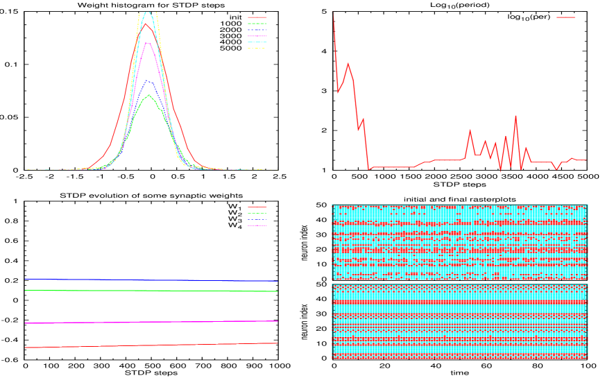
Figure 1: Effect of synaptic plasticity on: (up left) synaptic weights histogram; (up right) Period of the orbit; (down left) some synaptic weights evolution; (down right) raster plot of a few neurons.

References

- [1] E. L. Bienenstock, L. Cooper, and P. Munroe. Theory for the development of neuron selectivity: orientation specificity and binocular interaction in visual cortex. The Journal of Neuroscience, 1982.
- [2] T.V.P Bliss and A.R. Gardner-Medwin. Long-lasting potentiation of synaptic transmission in the dentate area of the unanaesthetised rabbit following stimulation of the perforant path. J Physiol, 232:357–374, 1973.
- [3] S.M. Dudek and M. F. Bear. Bidirectional long-term modification of synaptic effectiveness in the adult and immature hippocampus. J Neurosci., 1993.
- [4] A. Artola, S. Bröcher, and W. Singer. Different voltage-dependent thresholds for inducing long-term depression and long-term potentiation in slices of rat visual cortex. Nature, 1990.
- [5] W.B. Levy and D. Stewart. Temporal contiguity requirements for long-term associative potentiation/depression in the hippocampus. Neuroscience, 1983.
- [6] H. Markram, J. Lübke, M. Frotscher, and B. Sakmann. Regulation of synaptic efficacy by coincidence of postsynaptic ap and epsp. Science, 275(213), 1997.
- [7] G. Bi and M. Poo. Synaptic modification by correlated activity: Hebb’s postulate revisited. Annual Review of Neuroscience, 2001.
- [8] R. C. Malenka 1 and R. A. Nicoll. Long-term potentiation–a decade of progress? Science, 1999.
- [9] D.O. Hebb. The organization of behavior. New York: Wiley, 1949.
- [10] P. Dayan and L. F. Abbott. Theoretical Neuroscience : Computational and Mathematical Modeling of Neural Systems. MIT Press, 2001.
- [11] W. Gerstner and W. M. Kistler. Mathematical formulations of hebbian learning. Biol Cybern, 87:404–415, 2002.
- [12] L.N. Cooper, N. Intrator, B.S. Blais, and H.Z. Shouval. Theory of cortical plasticity. World Scientific, Singapore, 2004.
- [13] C. von der Malsburg. Self-organisation of orientation sensitive cells in the striate cortex. Kybernetik, 1973.
- [14] KD Miller, JB Keller, and MP Stryker. Ocular dominance column development: analysis and simulation. Science, 1989.
- [15] E.M. Izhikevich and N.S. Desai. Relating stdp to bcm. Neural Computation, 15:1511–1523, 2003.
- [16] B. Cessac, H.Rostro-Gonzalez, J.C. Vasquez, and T. Vieville. To which extend is the ”neural code” a metric ? In Neurocomp 2008, poster, 2008.
- [17] F. Rieke, D. Warland, Rob de Ruyter von Steveninck, and William Bialek. Spikes, Exploring the Neural Code. The M.I.T. Press, 1996.
- [18] P. Dayan and M. Hausser. Plasticity kernels and temporal statistics. Cambridge MA: MIT Press, 2004.
- [19] R. P. N. Rao and T. J. Sejnowski. Predictive sequence learning in recurrent neocortical circuits. Cambridge MA, MIT Press, 1991.
- [20] R. P. N. Rao and T. J. Sejnowski. Spike-timing-dependent hebbian plasticity as temporal difference learning. Neural Computation, 2001.
- [21] S. M. Bohte and M. C. Mozer. Reducing the variability of neural responses: A computational theory of spike-timing-dependent plasticity. Neural Computation, 2007.
- [22] G. Chechik. Spike-timing-dependent plasticity and relevant mutual information maximization. Neural Computation, 2003.
- [23] T. Toyoizumi, J.-P. Pfister, K. Aihara, and W. Gerstner. Generalized bienenstock-cooper-munro rule for spiking neurons that maximizes information transmission. Proc. Natl. Acad. Sci. USA, 2005.
- [24] T. Toyoizumia, J.-P. Pfister, K. Aihara, , and W. Gerstner. Optimality model of unsupervised spike-timing dependent plasticity: Synaptic memory and weight distribution. Neural Computation, 19:639–671, 2007.
- [25] M. Samuelides and B. Cessac. Random recurrent neural networks. EPJ Special Topics ”Topics in Dynamical Neural Networks : From Large Scale Neural Networks to Motor Control and Vision”, 142(1):89–122, 2007.
- [26] H. Soula and C. C. Chow. Neural Computation, Stochastic Dynamics of a Finite-Size Spiking Neural Networks.
- [27] B. Cessac and M. Samuelides. From neuron to neural networks dynamics. EPJ Special topics: Topics in Dynamical Neural Networks, 142(1):7–88, 2007.
- [28] E. Daucé, M. Quoy, B. Cessac, B. Doyon, and M. Samuelides. Self-organization and dynamics reduction in recurrent networks: stimulus presentation and learning. Neural Networks, 11:521–533, 1998.
- [29] B. Siri, H. Berry, B. Cessac, B. Delord, and M. Quoy. Effects of hebbian learning on the dynamics and structure of random networks with inhibitory and excitatory neurons. Journal of Physiology (Paris), 101((1-3)):138–150, 2007. e-print: arXiv:0706.2602.
- [30] B. Siri, H. Berry, B. Cessac, B. Delord, and M. Quoy. A mathematical analysis of the effects of hebbian learning rules on the dynamics and structure of discrete-time random recurrent neural networks. Neural Computation, 2008. to appear.
- [31] H. Soula. Dynamique et plasticité dans les réseaux de neurones à impulsions. PhD thesis, INSA Lyon, 2005.
- [32] H. Soula, G. Beslon, and O. Mazet. Spontaneous dynamics of asymmetric random recurrent spiking neural networks. Neural Computation, 18(1), 2006.
- [33] B. Cessac. A discrete time neural network model with spiking neurons. rigorous results on the spontaneous dynamics. Journal of Mathematical Biology, 56(3):311–345, 2008.
- [34] B. Cessac and T. Viéville. On dynamics of integrate-and-fire neural networks with adaptive conductances. Frontiers in Neuroscience, 2(2), July 2008.
- [35] G. Keller. Equilibrium States in Ergodic Theory. Cambridge University Press, 1998.
- [36] M.W. Hirsch. Convergent activation dynamics in continuous time networks. Neur. Networks, 2:331–349, 1989.
- [37] E. Schneidman, M.J. Berry, R. Segev, and W. Bialek. Weak pairwise correlations imply strongly correlated network states in a neural population. Nature, page 04701, April 2006.
- [38] G. Tkacik, E. Schneidman, MJ. Berry II, and W Bialek. Ising models for networks of real neurons. q–bio.NC/0611072, 2006.
- [39] S. Nirenberg and P. Latham. Decoding neuronal spike trains: how important are correlations. Proceeding of the Natural Academy of Science, 2003.