Optical Spectroscopy of X-ray sources in the Extended Chandra Deep Field South111This paper includes data gathered with the 6.5 meter Magellan Telescopes located at Las Campanas Observatory, Chile. 222Partly based on observations collected at the European Southern Observatory, Chile, under programs 078.A-0485 and 072.A-0139.
Abstract
We present the first results of our optical spectroscopy program aimed to provide redshifts and identifications for the X-ray sources in the Extended Chandra Deep Field South. A total of 339 sources were targeted using the IMACS spectrograph at the Magellan telescopes and the VIMOS spectrograph at the VLT. We measured redshifts for 186 X-ray sources, including archival data and a literature search. We find that the AGN host galaxies have on average redder rest-frame optical colors than non-active galaxies, and that they live mostly in the “green valley”. The dependence of the fraction of AGN that are obscured on both luminosity and redshift is confirmed at high significance and the observed AGN space density is compared with the expectations from existing luminosity functions. These AGN show a significant difference in the mid-IR to X-ray flux ratio for obscured and unobscured AGN, which can be explained by the effects of dust self-absorption on the former. This difference is larger for lower luminosity sources, which is consistent with the dust opening angle depending on AGN luminosity.
Subject headings:
galaxies: active – quasars: general – X-rays: galaxies1. Introduction
X-ray surveys have been critical in unveiling a large population of obscured supermassive black holes actively accreting matter (e.g., Giacconi et al., 2001 and references therein), contrary to optical surveys, like the Sloan Digital Sky Survey (e.g., Schneider et al., 2002), which are dominated by unobscured Active Galactic Nuclei (AGN). The hard spectral shape of the X-ray Background (XRB; e.g. Gruber, 1992) reveals that obscured AGN should significantly outnumber the unobscured sources, as was first proposed by Setti & Woltjer (1989). Given the difficulties in detecting and identifying the low luminosity and/or high redshift AGN, in particular those heavily obscured, it has been very challenging to obtain a complete census of the AGN population. This is particularly important in order to study the growth of supermassive black holes and its relation to the formation and evolution of its host galaxy.
Deep X-ray surveys like the Chandra Deep Fields North (CDF-N; Brandt et al., 2001) and South (CDF-S; Giacconi et al., 2001; Rosati et al., 2002) have been critical in obtaining a significant sample of obscured AGN up to significant distances. The first results from the optical follow-up of the X-ray sources in the Chandra Deep Fields reported a peak of the AGN activity at 0.7 (Szokoly et al., 2004), in contradiction with the predictions of the early XRB population synthesis (e.g., Comastri et al., 1995; Gilli et al., 2001), which expected a redshift peak at 1.5. This discrepancy was resolved in the XRB population synthesis models of Treister & Urry (2005) and later by Gilli et al. (2007), both of whom incorporated the latest Chandra and XMM-Newton observational results in their calculations. Similarly, the observed fraction of obscured to unobscured AGN in the Chandra Deep Fields was 1-2:1, lower than the value of 3-4:1 expected from XRB population synthesis models and observed in samples of nearby sources (Risaliti et al., 1999). This was explained by Treister et al. (2004) as due to the difficulty in obtaining spectroscopic identifications for obscured AGN at significant redshifts, which are much fainter in the optical than the unobscured sources.
One significant problem of these deep multiwavelength surveys is caused by the effects of cosmic variance. For example, Gilli et al. (2005) found a factor of two difference between the correlation length for AGN derived in the CDF-N and CDF-S fields, each covering 0.1 deg2, and concluded that this difference could be explained by the effects of cosmic variance. In addition, significant overdensities and large scale structures have been found in both fields (e.g., Gilli et al., 2003), which potentially affect the conclusions derived from each field individually. In order to address this problem, recently several wide-field deep surveys have been carried out. Examples of these surveys are the All-wavelength Extended Groth strip International Survey (AEGIS; Davis et al., 2007), the Cosmic Evolution Survey (COSMOS; Scoville et al., 2007) and the Multiwavelength Survey by Yale-Chile (MUSYC; Gawiser et al., 2006a; Treister et al., 2007). The Extended Chandra Deep Field South (ECDF-S) is one of the four 30′30′ fields studied by MUSYC. This field is 3 larger than the existing CDF-N or CDF-S. Hence, while the effects of cosmic variance are reduced compared to the results of each of these deep fields, the uncertainty due to large scale structure can still be relevant for our results. To minimize these effects, when possible, we combine in this work our data with available measurements in other fields.
Deep optical imaging has been obtained in the ECDF-S, mostly using the Wide Field Imager (WFI) on the 2.2-metre telescope at La Silla. Images in a narrow band filter centered at 500 nanometers were also obtained in this field in order to look for Lyman Alpha Emitters at 3 (Gawiser et al., 2006b). The ECDF-S imaging was made public by the ESO Deep Public Survey (Mignano et al., 2007), COMBO-17 (Wolf et al., 2004), and Garching-Bonn Deep Survey (GaBODS; Hildebrandt et al., 2006) teams. Deep near-IR coverage was obtained using the CTIO 4-metre telescope with the Infrared Sideport Imager (ISPI), reaching a magnitude limit of 22 (AB) in the bands333Optical and near-IR images and catalogs are public and can be obtained at http://www.astro.yale.edu/MUSYC. (E. Taylor et al. in prep.). In addition, the ECDF-S is the target of two Spitzer legacy surveys, the Spitzer IRAC / MUSYC Public Legacy in ECDF-S (SIMPLE) and the Far-Infrared Deep Extragalactic Legacy Survey (FIDEL), which obtained deep mid-IR data from 3 to 70 microns. Most relevant for our work is the Chandra coverage of the ECDF-S, consisting of 4 ACIS-I pointings centered on the original CDF-S to a depth of 230 ksec and covering an area of 0.3 deg2. A detailed description of these data was presented by Lehmer et al. (2005) and Virani et al. (2006). In this work we use the Virani et al. (2006) catalog for the optical follow-up. A total of 651 sources are included in this catalog to a flux limit of 1.710-16 erg cm-2s-1 in the 0.5-2 keV band. These sources constitute the main sample of this work.
In this paper we present the first results of an extensive spectroscopic effort aimed to identify a significant number of the X-ray sources in the ECDF-S field. Optical spectroscopy allow us to measure redshifts, and hence luminosities, and also to provide an indication of the nature of the source, which can be compared with the observed multiwavelength properties. In addition, we will focus on the properties of the obscuring material by studying the mid-IR properties of these sources, and by measuring the fraction of obscured AGN and its dependence on parameters like luminosity or redshift. In Section 2 we present the spectroscopic data and outline the reduction techniques used in this work, while in §3 the results are presented. In Section 4 we take advantage of the exquisite multiwavelength coverage available on the ECDF-S to compare the X-ray, optical and mid-IR properties of these sources. We also study the statistical properties of these sources in order to understand the evolution and physical conditions of the AGN population. The conclusions of our work are presented in §5. When required, we assume a CDM cosmology with =0.7, =0.3 and =0.7, in agreement with the most recent cosmological observations (Spergel et al., 2007). All magnitudes in this paper are presented in the AB photometric system (Oke & Gunn, 1983).
2. Optical Spectroscopy
Sources targeted for spectroscopy were selected from the catalog of Chandra sources of Virani et al. (2006). We use this catalog instead of a similar one presented by Lehmer et al. (2005) since the former uses a more detailed rejection of high-background periods, thus eliminating spurious sources. The Virani et al. (2006) catalog consists of 651 X-ray detected sources, 587 detected at high significance (the primary catalog) and 64 found using a lower threshold (secondary catalog). The X-ray sources were then matched to the MUSYC BVR optical catalogue presented by Gawiser et al. (2006b) using a likelihood ratio technique, as described by Cardamone et al. (2008), using a reliability threshold of 0.6. The estimated number of false matches using this technique, calculated by randomly changing the X-ray positions, is 1%. We found optical counterparts for 445 X-ray sources in the primary catalog (76%) and 28 in the secondary catalog (44%) down to a limiting magnitude of BVR=27.1. Using the Spitzer IRAC observations of the ECDF-S described in §2.5 and a similar likelihood ratio method we found near-IR counterparts for 554 (94%) X-ray sources in the primary catalog and 43 (67%) in the secondary catalog. Hence, we are very confident that a very large fraction of the X-ray sources, 90% in the primary and 70% in the secondary catalogs, are real.
While in principle all X-ray sources with optical counterparts were targeted for spectroscopy, we gave higher priority to the optically brightest sources, in order to increase the efficiency of our observations. In general, sources with 24 had a higher priority, except for our VIMOS (VLT Visible Multi-Object Spectrograph) observations, in which an 25 threshold was used. A total of 235 sources with 24 and 292 with 25 were targeted. As an experiment, for our IMACS (Inamori Magellan Areal Camera and Spectrograph) run of November 2005 we gave a higher priority to a group of 70 X-ray sources with bright optical counterparts (24) and a hard X-ray spectrum, given by a hardness ratio (HR) lower than -0.2. This was done in order to see if these sources have signs of obscuration in the optical spectrum as well, and to try to partially overcome the bias against obscured sources in identification studies based in optical spectroscopy. All these possible selection effects are considered on the analysis presented in §4.
2.1. Magellan IMACS data
We used the IMACS wide-field spectrograph mounted on the Magellan I Baade telescope at Las Campanas Observatory. This camera provides a circular field of view with a 27.2′ radius in the configuration. The pixel scale for this setup is 0.2′′/pixel. For all our observations we used the 300 lines/mm grism and slits of 1.2′′ width, except for the October 2003 and 2006 runs in which we used 1′′ slits. For our average seeing of 1′′, this translates into resolution elements of 8Å (6.5Å for the October 2003 and 2006 runs) except for the November 2005 run in which the average 0.6′′ seeing means a resolution element of 4Å for unresolved sources. While the wavelength coverage depends strongly on the position of the source in the mask, we required a minimum wavelength coverage of 4200-7000Å , which maximizes the number of sources on a given mask while at the same time providing a broad wavelength coverage, which is important considering that the redshifts are not know a priori and can span a wide range. The log of our ECDF-S IMACS observations is presented in Table 1.
Typically each mask was observed for 5 hours. The goal was to reach a magnitude of R24, however in many cases, due to weather or technical problems, this was not possible. Hence, the efficiency, defined as the fraction of sources identified and with a measured redshift, differs significantly from mask to mask. The total number of sources on a typical mask is 80-100, of which 15-50% are X-ray sources. The large spread in the fraction of X-ray sources on a given mask reflects the fact that these sources were not always the main target of the observations, but “mask-fillers”. The remaining targets include extragalactic sources like Ly- emitters, Lyman break galaxies and galactic white and brown dwarf stars selected by their optical colors from the MUSYC catalogues. The properties of the general sources targeted with IMACS will be presented in a following paper (P. Lira et al. in prep.).
2.2. VLT VIMOS data
The VIMOS (LeFevre et al., 2003) spectrograph mounted at the Nasmyth focus B of UT3 was also used to obtain optical spectroscopy for the X-ray sources in the ECDF-S. This instrument consists of four cameras of 7′8′ each, hence providing a total field of view of 15′16′, with a pixel scale of 0.2′′/pixel. We used the MR grism together with the OS-blue filter in order to block the contamination from higher orders. In this setup the wavelength coverage is 4000-6700Å , very similar to the coverage of the IMACS observations. This coverage minimizes the effects of fringing at red wavelengths and takes advantage of the wavelength region of maximum efficiency of the VIMOS camera. The MR grism provides a dispersion of 2.5Å /pixel, which combined with our 1′′ wide slits corresponds to a resolution element of 12.5Å . All the VIMOS observations were carried out in service mode by the Paranal staff. The required conditions were seeing better than 1′′, clear sky and fractional lunar illumination smaller than 20% at a minimum distance of 30 degrees. Due to the lack of an Atmospheric Dispersion Corrector in VIMOS and in order to minimize the effects of instrument flexures, observations were carried out at a maximum hour angle of 2 hours.
Four pointings were used to completely cover the ECDF-S 30′30′ field. Each mask was observed for three hours and 18 minutes, which corresponds to a total execution time of six hours including overheads. According to the exposure time calculator this should allow us to significantly detect sources up to R24.5. A total of 283 sources were targeted, excluding alignment stars, 96 of them X-ray sources.
2.3. Additional Observations
Since the ECDF-S is the target of many deep multiwavelength observations, it is not surprising that many spectroscopic follow-up programs have been carried out in this field. In order to take advantage of existing observations of these X-ray sources, we did an extensive literature search. In particular, we used the Master Compilation of GOODS/CDF-S spectroscopy444Available at http://www.eso.org/science/goods/spectroscopy/CDFS_Mastercat/. We matched this spectroscopic catalog to our MUSYC optical catalog using a search radius of 0.7′′. Then, we used the MUSYC-Chandra matched catalog described before and found spectroscopic identifications for the X-ray sources in the observations reported by Vanzella et al. (2005, 2006, 2008), Le Fèvre et al. (2004), Szokoly et al. (2004) and Croom et al. (2001). In total, existing identifications of 55 X-ray sources were added to our sample.
We also searched for existing unpublished spectroscopic observations in the ESO-VLT archive555The ESO archive can be found at http://archive.eso.org. We focused on VIMOS, given the large area covered by this camera and that most of the existing FORS2 observations were already incorporated in the master compilation described above. There are several VIMOS observations of the ECDF-S on the ESO archive, however of particular relevance for us was the program of Bergeron et al. (program ID 072.A-0139), for which 23 hours were granted in order to obtain spectroscopy of the X-ray sources detected by XMM. The area covered by XMM is well matched to the ECDF-S Chandra observations, so it is reasonable that a significant number of our Chandra sources were identified as part of this program. Three fields covered by the Bergeron program overlap with the ECDF-S. These fields were observed using both the MR and LR-Blue grisms with the GG475 and OS-Blue filters respectively. We looked for counterparts of our Chandra sources using a search radius of 2′′, which was chosen in order to account for the XMM positional uncertainty but at the same time avoid mis-identifications. In total, 36 sources in our Chandra catalog were observed as part of the Bergeron program; 28 of them were already targeted as part of our IMACS and VIMOS program, but only 11 successfully identified, so potentially identifications for 25 new sources could be obtained from the archival data.
2.4. Data Reduction
The IMACS data were reduced using the Carnegie Observatories System for MultiObject Spectroscopy (COSMOS) package666This software can be obtained from http://www.ociw.edu/Code/cosmos developed by Gus Oemler. This software was specifically designed to reduce IMACS data, in particular handling the challenge of having spectra spread over several CCDs. We followed the standard reduction cookbook, which consists of the following steps: construction of the spectral map using arc frames, bias-subtraction and flat fielding of science data and sky subtraction. We used COSMOS to generate 2D sky-subtracted wavelength-calibrated spectra of each source. We then used IRAF’s apall task in order to extract the 1D spectrum.
To reduce the VIMOS data we used the ESO VIMOS pipeline version 2.1.6777This package can be obtained from http://www.eso.org/projects/dfs/dfs-shared/web/vlt/vlt-instrument-pipelines.html. In this case all the spectra for a given quadrant are located on one CCD, so the data reduction is significantly simpler than for IMACS data. However, the basic reduction steps are very similar to the IMACS reduction. The same procedure was used to reduce both the archival observations and our proprietary data. In the case of the VIMOS data from our program, for each individual observation of 33 minutes, the corresponding night-time arc was used to calculate the spectral map, in order to account for the effects of instrument flexures. In addition, observations of standard stars on the same night were used to calculate the effective response as a function of wavelength for these observations.
2.5. Spitzer Data
In order to study the IR to X-ray ratio for our sample of sources with measured spectroscopic redshifts in the ECDF-S we took advantage of the deep Spitzer images available in this field. At the shortest wavelengths, the central CDF-S region (10′16′) was observed by IRAC (Fazio et al., 2004) as part of the GOODS survey to flux limits of 0.13, 0.22, 1.45 and 1.61 Jy in the 3.6, 4.5, 5.7 and 8 m band respectively. Source matching and basic IR properties were reported by Treister et al. (2006). In addition, the whole ECDF-S field was covered by IRAC as part of the SIMPLE survey888Further information about this survey, catalogs and images can be found at the website http://www.astro.yale.edu/dokkum/simple/ (Damen et al. in prep.). The flux limits for the SIMPLE observations are 0.76, 0.4, 5.8 and 3.6 Jy in the 3.6, 4.5 and 5.7 and 8 m bands respectively, thus 3-5 shallower than the GOODS observations. The matched catalog of the ECDF-S X-ray sources to the SIMPLE images used here was presented and described in detail by Cardamone et al. (2008).
At longer wavelengths, we use the available Spitzer MIPS (Rieke et al., 2004) observations at 24 m. In the central region, GOODS provide deep images to a flux limit of 25 Jy. A catalog999More details about this catalog and data-reduction procedures can be found at the webpage http://data.spitzer.caltech.edu/popular/goods/Documents/goods_dataproducts.html based on PSF-fitting magnitudes, described by Treister et al. (2006) and R. Chary et al. (in prep.), was matched to the X-ray sources in the GOODS region using the IRAC-derived positions.
Additional data at 24 m covering the whole ECDF-S field were taken as part of the FIDEL survey. Unfortunately, at the moment only the reduced images were made available by the FIDEL group101010The reduced images and more details about the survey and reduction techniques can be found at http://data.spitzer.caltech.edu/popular/fidel/2007_sep17/fidel_dr2.html. In order to produce our own catalog based on the reduced FIDEL images we used the Mosaicking and Point-Source Extraction (MOPEX; Makovoz & Marleau, 2005) package, provided by the Spitzer Science Center. Briefly, we did a first-pass extraction using the default point response function (PRF) included in MOPEX in order to obtain a preliminary catalog of the brightest sources. These sources were then used to construct a customized PRF, based directly in the FIDEL observations. Finally, using this PRF we performed a second extraction and measured PRF-fitting flux densities for the detected sources. This procedure is described in more detail by Makovoz & Marleau (2005). In order to verify the accuracy of our derived fluxes in Figure 1 we compare the FIDEL and GOODS sources for the 829 overlapping sources with fluxes higher than 60 Jy in order to ensure a reliable detection in the FIDEL image. There is a very good agreement between the FIDEL and GOODS fluxes. The median ratio of FIDEL to GOODS flux is 0.97 with a standard deviation of 7%. Given the very small systematic offset between the FIDEL and GOODS fluxes, well within the measurement errors, no correction to the FIDEL fluxes was applied. The FIDEL catalog was matched to the ECDF-S using the maximum likelihood procedure described by Cardamone et al. (2008).

3. Results
A total of 339 X-ray sources in the Virani et al. (2006) catalog were targeted for spectroscopy using the VIMOS and IMACS spectrographs and data from the literature. For 186 of them, we were able to identify the nature of the source and measure the redshift, giving an average efficiency of 55%. Of those, 180 were detected in the high-significance primary X-ray catalog. The basic X-ray, optical and spectroscopic properties of these sources are presented in Table 2. The R-band magnitude distributions for all the X-ray sources, the sources targeted for spectroscopy and those with spectroscopic identification are presented in Figure 2. The fraction of sources that are successfully identified depends strongly on the observing conditions, achieved exposure time, etc. (Table 1). At the same time, this fraction always decreases strongly towards fainter magnitudes (Figure 2). In our analysis, we model this dependence using a very simple linear fit, with a constant value of 65% to =22 and then decreasing linearly to 0% at =26.5. The resulting fit is shown in the upper panel of Figure 2.

The redshift distribution for our spectroscopically-identified sources is presented in Figure 3. The vast majority of unobscured sources (that present broad emission lines, see discussion below) are at 1, with an average redshift of 2.22 and a median of 2.12. In contrast, obscured AGN and X-ray emitting galaxies are preferentially located at 1. For the total sample, the average redshift is 1.18, with a median of 0.75, in good agreement with the results found in both Chandra Deep Fields (Szokoly et al., 2004; Barger et al., 2003; Gilli et al., 2005). The highest redshift source in our sample is a broad line AGN, XID 213, at =4.48.

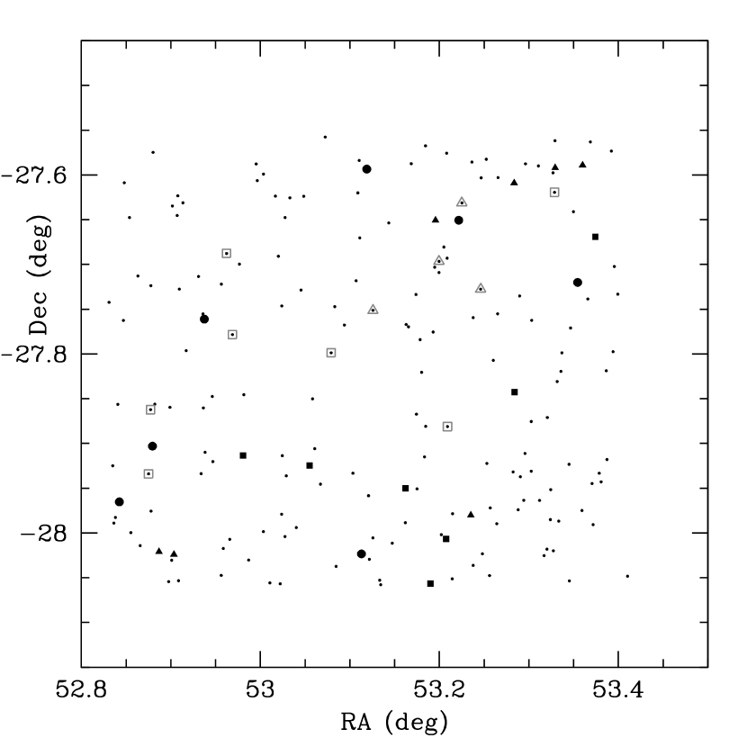
In the upper panel of Figure 3 we use a narrower bin width (=0.02), in order to search for structures in redshift space. The two main structures, “walls”, previously detected in the CDF-S proper at =0.67 and =0.73 (Gilli et al., 2003; Adami et al., 2005) are also easily found in our sample. In addition, we found excesses of sources at =0.15,0.29 and 0.53. In Figure 4 we present the spatial distribution of all the identified sources, with the position of the sources in those redshift structures highlighted. For =0.15,0.29 and 0.53 the 30′30′ ECDF-S field corresponds to a comoving area of 4.64.6, 7.77.7 and 11.211.2 Mpc2 respectively. Given that all the redshift groups span almost the whole field of view, these structures are much larger than the compact structures reported by Adami et al. (2005). In order to estimate the probability of having seven sources in one =0.02 bin we assume that the redshift distribution follows a Poisson distribution. The average number of sources in a =0.02 bin is 2. Hence, the probability of having seven sources in one bin randomly is 0.3%. Therefore, we can conclude that these groups in redshift space should correspond to real physical associations.
Sources were mainly classified according to their optical spectroscopy characteristics. Our primary division comes from the presence or absence of broad emission lines. The threshold for unobscured sources was set at v1000 km s-1, since Barger et al. (2005) showed that the vast majority of the non-X-ray sources have line-widths smaller than this value, while sources with broad lines have also soft X-ray spectra, consistent with being dominated by an unobscured AGN. We then used the hard (2-8 keV) X-ray luminosity to separate normal galaxies with X-ray emission from AGN-dominated sources. Specifically, we assumed a conservative and typical threshold of =1042erg s-1, higher than the highest level of X-ray activity observed in star-forming galaxies (e.g., Lira et al., 2002).
The X-ray spectral shape can be used to obtain an alternative source classification. In particular, the hardness ratio, defined as the ratio between the difference of the hard band (typically 2-8 keV for Chandra observations) and soft band (0.5-2 keV) count rates and their sum is used when the number of detected counts is not enough to perform X-ray spectral fitting. Figure 5 shows the hardness ratio as a function of luminosity for the 186 sources with spectroscopic identifications presented in this paper. As can be seen, sources with hard X-ray spectrum (positive hardness ratio) tend to be also optically classified as obscured sources in the optical, while sources that present broad emission lines have in general a soft X-ray spectrum (negative hardness ratio). It is also interesting that most of the unobscured sources, in both X-rays and optical wavebands, have a high X-ray luminosity (1043 erg s-1), while most obscured sources are fainter in X-rays. These trends will be studied in further detail in the following section.

While the hardness ratio can be used as a rough indication of the X-ray spectral shape, for the brighter X-ray sources it is possible to perform more accurate spectral fitting. In the case of the ECDF-S, a total of 184 sources have more than 80 counts detected in the 0.5-8 keV Chandra band, making spectral fitting possible. We used a modified version of the Yaxx111111Available at http://cxc.harvard.edu/contrib/yaxx/ software to extract the spectrum of each high-significance source. For sources with more than 200 background-subtracted counts and measured redshifts, 72 in the ECDF-S, we simultaneously fitted a power-law spectrum and photoelectric absorption, with three free parameters: slope of the power law (), normalization and observed neutral hydrogen column density (). In all cases we included the Galactic absorption, assuming an average of 6.81019 cm-2 for the ECDF-S, as measured by the survey of Galactic HI of Kalberla et al. (2005). For sources with less than 200 but more than 80 counts it was not possible to perform such detailed fitting, so we fixed the slope of the power-law to a value of =1.9, very similar to the average value for the sources with a fitted slope (=1.95), which also corresponds to the typical X-ray spectrum for unobscured AGN (Nandra & Pounds, 1994; Nandra et al., 1997 and others). In both cases, the value was derived in the observed frame, in order to keep the X-ray spectral fitting independent of the redshift measurements. In order to calculate the conversion from observed to intrinsic we used the Xspec version 12.4.0 software (Arnaud, 1996) to simulate a X-ray spectrum with =1.9 as observed at the Chandra aimpoint with ACIS-I, added absorption at varying redshifts from 0 to 4 and measured the fitted value in the observed frame. We obtained an empirical relation of (intr)=(1+)2.65(obs), consistent with the conversion assumed in the past for Chandra data (e.g., Bauer et al., 2004). Furthermore, we checked that the derived relation is roughly independent of the assumed slope of the power-law spectrum. Hence, we are very confident that our conclusions are not affected by our choice of measuring absorption in the observed frame.
The conversion from observed to intrinsic can thus only be done for sources with a measured redshift. We have spectroscopic redshifts, given in Table 2, for a total of 80 sources with fitted . However, in order to increase our sample we used the good quality photometric redshifts derived by the COMBO-17 survey, which provides redshifts accurate to /(1+)10% for sources with 24 (Wolf et al., 2004). This uncertainty in redshift translates into an uncertainty in the derived intrinsic of 0.12, smaller than the typical errors in the fitted observed or the bin size in our distribution (Fig. 6). Hence, it is acceptable to use the COMBO-17 photometric redshifts in order to convert observed into intrinsic values, thus increasing our sample to 144 sources. To confirm that the use of COMBO-17 redshifts does not bias our conclusions, we performed a Kolmogorov-Smirnov (KS) test and found that the hypothesis that both distributions were drawn from the same parent distribution can only be dismissed at the 0.02% confidence level.

4. Discussion
4.1. X-ray/Optical Classification
The bottom panel of Figure 6 shows the distribution of intrinsic separately for sources classified as obscured and unobscured AGN based only on optical spectroscopy. While the average value of is larger for obscured than unobscured sources, 81021 cm-2 versus 21021 cm-2, the difference is not very large. Performing a KS test to these two distributions rules out the hypothesis that they were drawn from the same parent distribution with a 98.5% confidence, leaving a small but not completely negligible probability. Since they are both indications of the X-ray spectral shape, there is a close relationship between the hardness ratio and derived values. As can be seen in Figure 7, for modest column densities, 1022.5 the values are very sensitive to small changes in the number of detected soft X-ray photons, in particular for high redshift sources. This implies that there can be large errors in the derived values, in particular for unobscured sources at high redshift. The implications of this potential bias in our analysis will be further discussed below.

As was shown in Figures 5 and 7, the optical and X-ray classifications do not always agree. In order to further investigate this effect, in the left panel of Fig. 8 we show the intrinsic versus hard X-ray luminosity, used as a tracer of the intrinsic AGN luminosity. For this figure we also added 335 X-ray sources detected in the 1 Msec. CDF-S observations with accurate measurements based on spectral fitting presented by Tozzi et al. (2006). Redshifts for those sources, either photometric or spectroscopic, were compiled by Zheng et al. (2004). This figure shows two interesting effects. At low luminosities, 1043 erg s-1, a large fraction of the sources optically classified as obscured AGN have intrinsic values lower than 1022 cm-2. This can be explained by the effects of dilution of the AGN light by the host galaxy (e.g., Moran et al., 2002; Cardamone et al., 2007), which lowers the equivalent width of the broad emission lines because of the relatively high continuum from the host galaxy, thus making a source to be erroneusly classified as obscured AGN in the optical. A second effect appears at high luminosity: sources optically classified as unobscured AGN have intrinsic values higher than 1022 cm-2. A possible explanation for this effect can be found in the right panel of figure 8, where we can see that the sources with discrepant X-ray/optical classifications are predominantly located at 2.5. Given the strong redshift dependence of the accuracy of determinations, sources with very small observed values, which can be in general explained by measurement errors, will have a high intrinsic values if the source is located at high redshift. At high redshift, the Chandra observations trace emission at higher energy in the rest frame, thus making it much harder to detect the photoelectric absorption cutoff, critical for measuring . This effect was already studied and simulated by Akylas et al. (2006), who found that at high redshift the derived column densities are systematically overestimated. According to the results of Akylas et al. (2006), measurements are systematically overestimated by 50% at 2.5 and 20% at 1.5.
An obvious conclusion of this analysis is that no classification method is perfect and can be used for all sources. An early attempt to use a combined X-ray/optical classification was performed by Szokoly et al. (2004). In their work, they used a separation between obscured and unobscured sources at a hardness ratio of -0.2. A similar approach was used by Hasinger et al. (2005) to select unobscured AGN from an X-ray selected samples. This threshold is shown in Figure 5 for the sources with spectroscopic identification in the ECDF-S. A hardness ratio of -0.2 corresponds to an intrinsic of 1022 cm-2 at =0.5, assuming =1.9, while sources with this at lower redshift will have a higher (more positive) value. So, a threshold of -0.2 in HR to separate obscured and unobscured AGN is appropriate at 0.5. However, as is clear from Figure 8, the effects of dilution by the host galaxy are important only for low luminosity sources, which are predominantly located at low redshift. Hence, we propose the following classification scheme: For sources at 0.5 we will separate obscured and unobscured sources at HR=-0.2, regardless of their optical properties, while for sources at higher redshifts we will use only the optical classification scheme, as measurements are biased at high redshift.
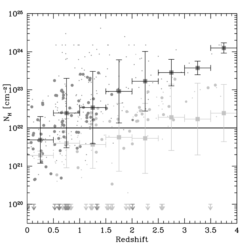
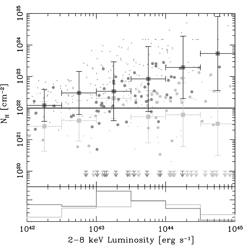
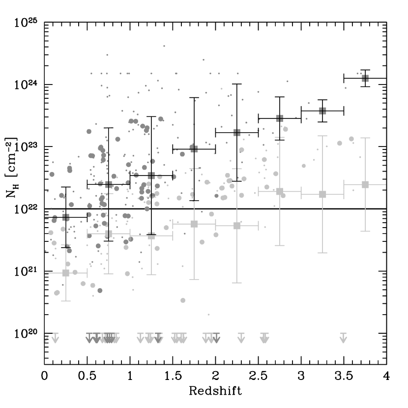
In Figure 9 we show the measured values as a function of luminosity and redshift for the new classification scheme. As expected, changes are relevant only for sources with low luminosities at low redshifts. With an optical classification only, the average for obscured sources at 0.5 is 4.81021 cm-2, while using the X-ray classification it is 7.31021 cm-2. Similarly, in the lowest luminosity bin, 3.21042 erg s-1, obscured and unobscured AGN are now clearly separated in . This separation is not even larger since heavily-obscured low-luminosity sources are preferentially missed by the X-ray observations, and thus not included in our sample.
4.2. Rest-frame Optical Colors
As is well known (e.g., Baldry et al., 2004; Weiner et al., 2005; Cirasuolo et al., 2007 and references therein), the distribution of optical colors in normal galaxies is bimodal, with a large population of blue star-forming galaxies in the blue cloud separated from the “red sequence” of massive passively-evolving spheroids. As was recently reported (e.g., Barger et al., 2003; Nandra et al., 2007; Georgakakis et al., 2008; Silverman et al., 2008), most galaxies hosting obscured AGN, in which the integrated optical light is dominated by the host galaxy (e.g., Treister et al., 2005), lie on the “green valley”, a transition region located between the red sequence and the blue cloud. Hence, this can be considered as good evidence for a link between AGN and galaxy evolution, possibly indicating that AGN feedback can play a role in regulating star formation (Springel et al., 2005; Schawinski et al., 2006); however, this remains controversial, as discussed by Alonso-Herrero et al. (2008).
To compute the rest-frame optical colors for the X-ray sources with spectroscopic identification on the ECDF-S field we started from the MUSYC optical catalog of Gawiser et al. (2006b). In order to increase the number of sources in our sample we added the X-ray sources with reliable photometric redshifts from the COMBO-17 survey, as described before. We then generated the rest-frame spectral energy distribution for each X-ray source with measured redshift by interpolating the observed photometric data points. The rest-frame and optical magnitudes were then computed by convolving the energy distribution with the corresponding filter response. The resulting rest-frame - colors versus , the rest-frame -band absolute magnitude, are shown in Fig. 10. A significant number of X-ray sources have -1 and -22. In general, those sources were classified as unobscured AGN because of the presence of broad emission lines. Since the optical continuum of these sources is dominated by the AGN and not the host galaxy, we exclude them from further analysis. However, as it was found by Schawinski et al. (2008), once the emission from the central source is removed, the host galaxies of unobscured AGN have optical colors similar to those of unobscured AGN. As can be seen by comparing with a population of normal galaxies obtained on the same field from the COMBO-17 survey, the X-ray sources classified as obscured AGN have in general redder optical colors than normal galaxies and lie outside of the main blue cloud.
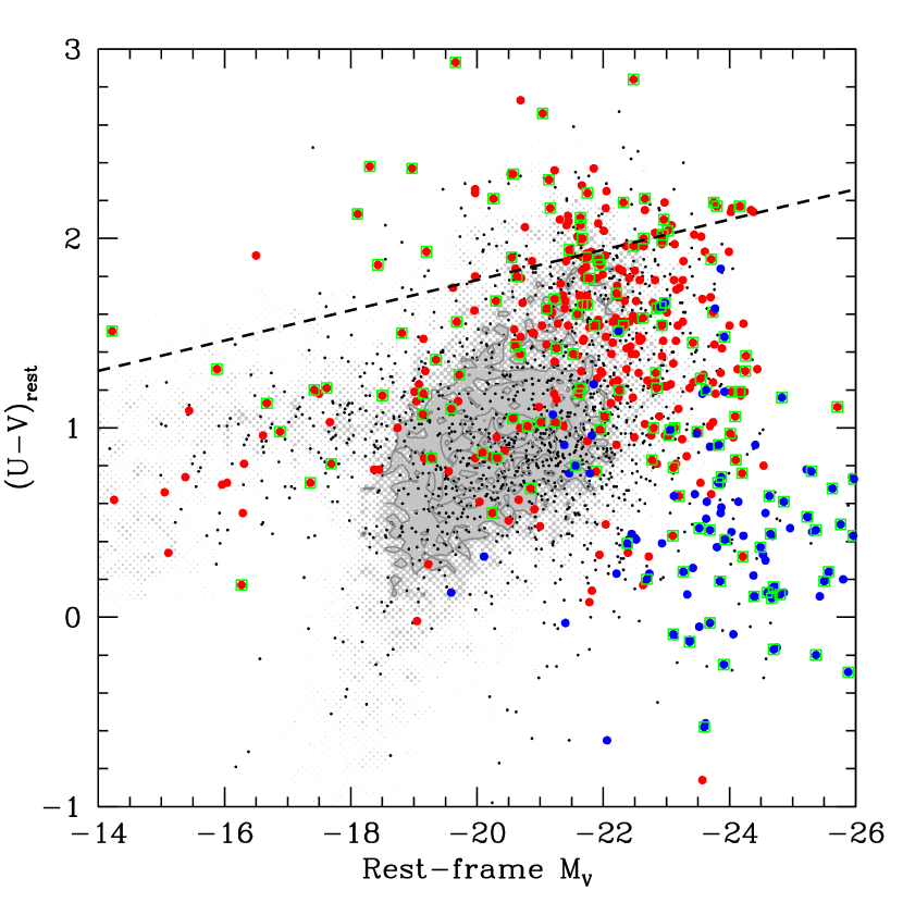
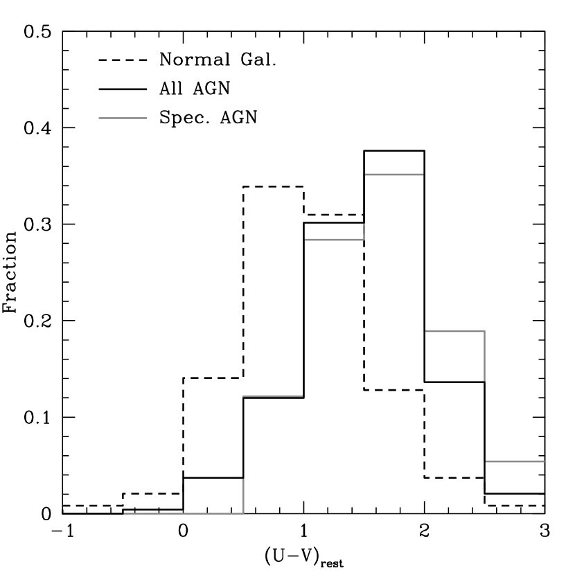
The excess of red sources in the AGN population can be easily seen in Fig. 11, where the distributions of rest-frame - colors for X-ray emitting sources and normal galaxies are presented. In order to limit the influence of differences in the sample selection, the comparison sample was obtained randomly from the ECDF-S inactive galaxies to match the AGN redshift distribution. Performing a KS test we found that the probability that these two distributions were drawn from the same parent distribution is negligible. Contrarily, a KS test comparing the distribution of the X-ray sources with spectroscopic and photometric redshift returned a relatively high probability of 20%, indicating that the use of photometric redshifts does not significantly bias our results. The fact that results of the KS test are not even higher can be explained since in general sources with spectroscopic redshifts have brighter optical counterpart, and thus slightly different average - colors. However, this is a minor effect that will not affect our conclusions.
Given that the comparison sample was selected to have the same absolute optical magnitude and redshift distributions as the AGN host galaxies, it is unlikely that the differences in optical colors are due to the sample selection. A similar analysis was performed by Georgakakis et al. (2008) using the AGN detected in the AEGIS survey. Studying the morphology of AGN host galaxies, they found only a small fraction of major mergers, but evidence of minor interactions in a large number of sources. Both Georgakakis et al. (2008) and Schawinski et al. (2008) concluded that AGN activity should outlive the truncation of star formation, in order to explain the observed red optical colors of AGN host galaxies.
4.3. Obscured AGN Fraction
The fraction of obscured AGN and its possible dependence on parameters like redshift or luminosity is very important for AGN population studies, in particular given its direct relation with our understanding of the cosmic X-ray Background. A dependence of the obscured fraction on luminosity was previously found for X-ray selected samples by Ueda et al. (2003), Steffen et al. (2003), La Franca et al. (2005) and Treister et al. (2005) among others. A physical explanation, proposed by Lawrence (1991) and updated by Simpson (2005), is the so-called “receding torus”. More recently, Treister et al. (2008) found a dependence of the ratio of mid-IR to bolometric flux on luminosity for unobscured AGN consistent with an increase in the opening angle with luminosity. Similarly, Akylas & Georgantopoulos (2008) proposed that the observed dependence of the obscured fraction on luminosity could be explained by the effects of photo-ionization on the X-ray obscuring matter, while Hönig & Beckert (2007) argues that the effects of the Eddington limit on a clumpy torus can explain the observed luminosity dependence of the obscured AGN fraction. The large sample of X-ray sources in the ECDF-S can be used to further explore this luminosity dependence of the obscured AGN fraction. In figure 12 we can see that using the ECDF-S sample alone the fraction of obscured AGN decreases from 90% at 1043 erg s-1 to 20% at =1045 erg s-1, using the “hybrid” classification scheme described in §4.1.
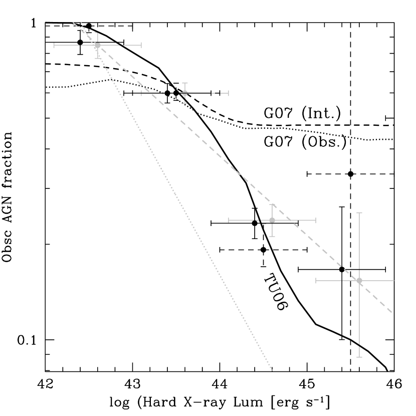
In order to increase the significance of this result, we added the results from the ECDF-S to the compilation presented by Treister & Urry (2006), which combined the results from seven X-ray surveys ranging from wide area shallow surveys to the Chandra deep fields. The total sample includes now 2814 X-ray sources, 1377 (49%) of them with spectroscopic identification. In Figure 12 we present the resulting obscured AGN fraction as a function of luminosity for the total sample. The obscured fraction ranges from 807% at 1043 erg s-1 to 168% for 1045 erg s-1. In addition, Figure 12 shows the predicted luminosity dependence incorporated in the Treister & Urry (2005) AGN population synthesis model, as updated by Treister & Urry (2006) to include a redshift dependence, and for comparison the luminosity dependence used in the models of Gilli et al. (2007). While at low luminosities both models agree well with the observations, for luminosities higher than 1044 erg s-1 the Gilli et al. (2007) models predict a fraction of obscured AGN of 50%, significantly higher than the observed value. This discrepancy has important consequences for the modeling of the X-ray background using AGN, as the largest contribution comes from sources at roughly these luminosities (e.g., Treister & Urry, 2005). The larger fraction assumed by Gilli et al. (2007) is more relevant at lower energies, where the effects of absorption are larger. For example, the XRB intensity at E10 keV in the Gilli et al. (2007) model is 40% lower than the Treister & Urry (2005) calculation, while it is now clear from recent Chandra and XMM observations (De Luca & Molendi, 2004; Hickox & Markevitch, 2006) that a larger XRB intensity at low energies is more appropriate.
In addition, in Figure 12 we compare the observed dependence of the fraction of obscured sources on luminosity with the expectations for different geometrical parameters of the obscuring material. If the height of the torus is roughly independent of luminosity, the change in covering fraction is due to a change in inner radius (the original “receding torus” model), hence a rough dependence for the contrast should be expected (Barvainis, 1987; Lawrence, 1991). If the effects of radiation pressure are incorporated, in the case of a clumpy torus, Hönig & Beckert (2007) derive a dependence for the contrast. As can be seen in Figure 12, a dependence is too steep compared to observed data. This implies that the height of the obscuring material cannot be independent of the source luminosity and provides evidence for a radiation-limited structure, as the one suggested by Hönig & Beckert (2007).
The dependence of the fraction of obscured AGN on redshift is more controversial. While some studies (e.g., La Franca et al., 2005; Ballantyne et al., 2006; Treister & Urry, 2006; Della Ceca et al., 2008) found a small increase in the fraction of obscured AGN at higher redshifts, other results suggest that this fraction is constant (e.g., Ueda et al., 2003, Akylas et al., 2006). The upper panel of Fig. 13 shows the observed fraction of obscured AGN as a function of redshift for the sources in the ECDF-S. This fraction is high, 90%, at 1, while at higher redshifts it decreases to 30-40%. As for the luminosity dependence, in order to increase the significance of our results we added the ECDF-S sources to the sample of Treister & Urry (2006). The results for the large sample are consistent with those from the ECDF-S alone; namely, at low redshift there is a large fraction of obscured sources with a steep decline at 1. This decline in the observed fraction of obscured sources can be easily explained by a simple observational fact: in order to be included in this sample a source needs to have a measured redshift from optical spectroscopy. For obscured AGN, the optical light is dominated by the host galaxy (e.g., Barger et al., 2005; Treister et al., 2005), which becomes too faint for spectroscopy with 8 meter class telescopes at 1. In order to quantify this effect, we use the ratio of identified to total X-ray sources in a given optical magnitude bin (upper panel, fig. 2). This magnitude-dependent ratio is used to calculate the expected obscured AGN fraction including the X-ray and optical flux limits and the luminosity dependence of the obscured fraction. This calculation is done as described in detail by Treister & Urry (2006). Briefly, we used the AGN population synthesis of Treister & Urry (2005), together with the library of AGN spectra described by Treister et al. (2004), and calculated the effective area of the survey as a function of both X-ray flux and optical magnitude, taking into account the spectroscopic incompleteness at each optical flux. This procedure outputs a expected number of observed obscured and unobscured AGN as a function of redshift, for a non-evolving obscured AGN fraction.
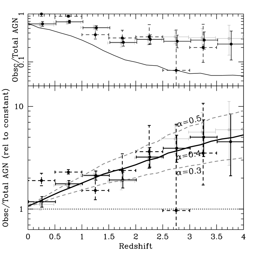
As can be seen in the upper panel of Figure 13, the expected decrease is actually steeper than what is observed. This implies that the inferred fraction of obscured AGN in the ECDF-S should increase with redshift, once the selection effects in the sample are accounted for. This dependence is consistent with the results of Treister & Urry (2006), who found that this increase can be represented as a power-law of the form (1+)α, with =0.40.1. These results are roughly independent of the method used to classify AGN; we obtained the same dependence using both our mixed X-ray/optical classification scheme and one based completely on optical spectroscopy.
4.4. Number Density and Evolution of AGN
Using our combined sample of X-ray selected AGN we can also compute the AGN spatial density as a function of redshift, and compare with the expectations from existing AGN luminosity functions based on smaller samples. In order to calculate the AGN spatial density, we started from our collected sample of 1377 sources described above. We then separated the sources in low (=1041.5-43 erg s-1), medium (=1043-44.5 erg s-1) and high luminosity (=1044.5-48 erg s-1) bins. For each luminosity class we binned the sample in redshift so that each bin has at least 50 sources (20 for the highest luminosity sources). Then, the spatial density of each bin was calculated by summing the values of for each source in the bin, where is the total comoving volume per unit area in that bin multiplied by the area covered by our super-sample at the X-ray flux of the source. In addition, upper limits for the spatial density on each bin were calculated by multiplying the values of by the fraction of spectroscopically identified sources at the optical magnitude of the AGN, as described in Treister & Urry (2006) for the general sample and in the upper panel of Fig. 2 for the ECDF-S.
In Fig. 14 we show the observed AGN spatial density as a function of redshift for low, medium and high luminosity sources compared with the expected density obtained from integrating the hard X-ray luminosity functions presented by Ueda et al. (2003), Barger et al. (2005) and La Franca et al. (2005). While the X-ray sources in these studies were selected in similar ways, the samples have different numbers of sources (247 AGN in Ueda et al., 2003, 746 in Barger et al., 2005, and 508 in La Franca et al., 2005) with the emphasis set at different flux levels (mostly bright sources in Ueda et al., 2003, moderate fluxes in La Franca et al., 2005 and faint sources in Barger et al., 2005). In addition, the modeling of the luminosity function is also different in these papers. While Barger et al. (2005) assumed pure luminosity evolution, both Ueda et al. (2003) and La Franca et al. (2005) found better results using a luminosity-dependent density evolution. As can be seen in Fig. 14, at high and moderate luminosities all the luminosity functions studied here agree well with the observations at low redshifts, while at high redshifts the expectations from both the Ueda et al. (2003) and La Franca et al. (2005) works are significantly above the observed values for intermediate luminosity sources.
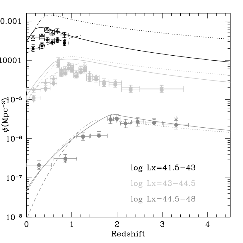
This discrepancy can most likely be explained by the effects of incompleteness in the X-ray data, which are particularly important for the lower luminosity sources. As it was concluded by e.g., La Franca & Cristiani (1997), the method used here is particularly sensitive to the effects of incompleteness. The work of Ueda et al. (2003) and La Franca et al. (2005) both used the / method, which attempts to account for incompleteness by using the expected number of sources in a given luminosity and redshift bin. One obvious caveat of this method is that the results are model dependent. We attempt to correct for incompleteness in the X-ray data, in the two lowest luminosity bins, where these effects are more important. In order to do that, we use the model described in the previous section in order to calculate the fraction of sources missed by the X-ray selection in a given luminosity and redshift bin due to the effects of obscuration. For the lowest luminosity sources, this correction is roughly 2, while at higher luminosities it is about 30-40%. We did not attempt to correct the highest luminosity bin, since the effects of absorption are negligible for these sources. As can be seen in Fig. 14, after the correction for incompleteness is applied a good agreement with the predicted spatial density using the luminosity function of Ueda et al. (2003) is found. The remaining discrepancy with the work of La Franca et al. (2005) could be explained because in this case even highly obscured Compton-thick AGN up to =1026 cm-2 are included, while in the case of Ueda et al. (2003) and in our work only mildly Compton-thick AGN with 1025 cm-2 are considered. Finally, it is worth mentioning that in the luminosity function of Barger et al. (2005) not attempts were made to correct for incompleteness in the X-ray selection. Hence, a good agreement is found only for the uncorrected data points.
4.5. Infrared (IR) to X-ray ratio
Emission at X-ray wavelengths, in particular in the hard band, is often used as a tracer for the direct AGN output mainly from Compton-scattered accretion disk photons, while the luminosity at longer wavelengths, in particular in the mid-far infrared, is associated with the re-radiation of the energy absorbed by the surrounding gas and dust (e.g., Pier & Krolik, 1993). There is currently a strong debate about the geometry and characteristics of this surrounding dust, in particular whether it has a smooth (e.g., Pier & Krolik, 1992) or clumpy (e.g., Krolik & Begelman, 1988) distribution. The ratio of IR to X-ray luminosity can be used to distinguish between these two distributions and to constrain the dust geometry (Lutz et al., 2004). For example, smooth torus models predict large differences in the IR to X-ray ratio for obscured and unobscured sources, due to the significant effects of self-absorption. Contrarily, radiation transfer models of clumpy dust torii predict very small or no differences between the IR to X-ray ratio for obscured and unobscured AGN.
The observational evidence remains controversial. The work of Horst et al. (2006) reports that no differences were found in the mid-IR (measured at a fiducial rest-frame wavelength of 12.3 m) to X-ray ratio for a sample of 17 nearby AGN observed with the VLT-VISIR, which provides a relatively high angular resolution of 0.35′′. In apparent contradiction, Ramos Almeida et al. (2007) found a slightly smaller value for the X-ray to nuclear mid-IR (at 6.75 m) ratio from a sample of 57 AGN. For the latter, the observations were carried out using the ISOCAM camera onboard ISO, with a more limited angular resolution of 4′′. Horst et al. (2008) argue that precisely this difference in angular resolution explains the discrepant results. Using their high spatial resolution images, they claim that the contribution from star formation, unresolved in the ISOCAM observations, can account for the observed differences between obscured and unobscured AGN. On the other hand, the relatively small sample of Horst et al. (2006) traces larger intrinsic luminosities for unobscured sources compared to the obscured sample, thus contributing to explain why no difference in the IR to X-ray ratio was found. Given the large scatter in the IR to X-ray ratio reported by both groups, a large sample of sources is required to reach statistically significant conclusions.
In Figure 15 we present the values of the ratio of to as a function of , the rest-frame wavelength. These values were computed using both the IRAC and MIPS fluxes, for the sources in our sample with Spitzer detections and measurements. We also added the sources in the central region with measured from the X-ray spectrum by Tozzi et al. (2006). In order to correct the hard X-ray (2–8 keV) luminosities, , for the effects of absorption we used the photoelectric absorption cross sections derived by Morrison & McCammon (1983) and the values measured from X-ray spectral fitting as described above. Given that the effects of X-ray absorption in sources classified as unobscured are typically very small, and those values can be significantly affected by measurement errors, we only corrected the X-ray luminosities of the obscured sources. If no correction for absorption is done to the X-ray luminosities of the obscured sources, our conclusions are unchanged. As can be seen in Fig 15, sources classified as obscured and unobscured AGN have significantly different average values of /, and this separation depends on wavelength. At the shortest wavelengths, 1 m, the separation in this ratio is rather small, which can be explained by the contribution of the stellar light of the host galaxy to the integrated emission. This effect remains visible until 2 m, where the stellar light starts to fade and emission from the host dust in the inner region of the surrounding material in the AGN begins to dominate. This emission is highly affected by self-absorption, as most torus models predict (see, e.g., Pier & Krolik, 1993; Nenkova et al., 2002; Hönig et al., 2006), thus explaining why at these wavelengths unobscured sources have significantly higher values of /. At longer wavelengths, 10 m, the contrast between obscured and unobscured sources is reduced again, since the optical depth is reduced at longer wavelengths. Thus, it is expected that at 30-40 m the IR emission should become isotropic again.
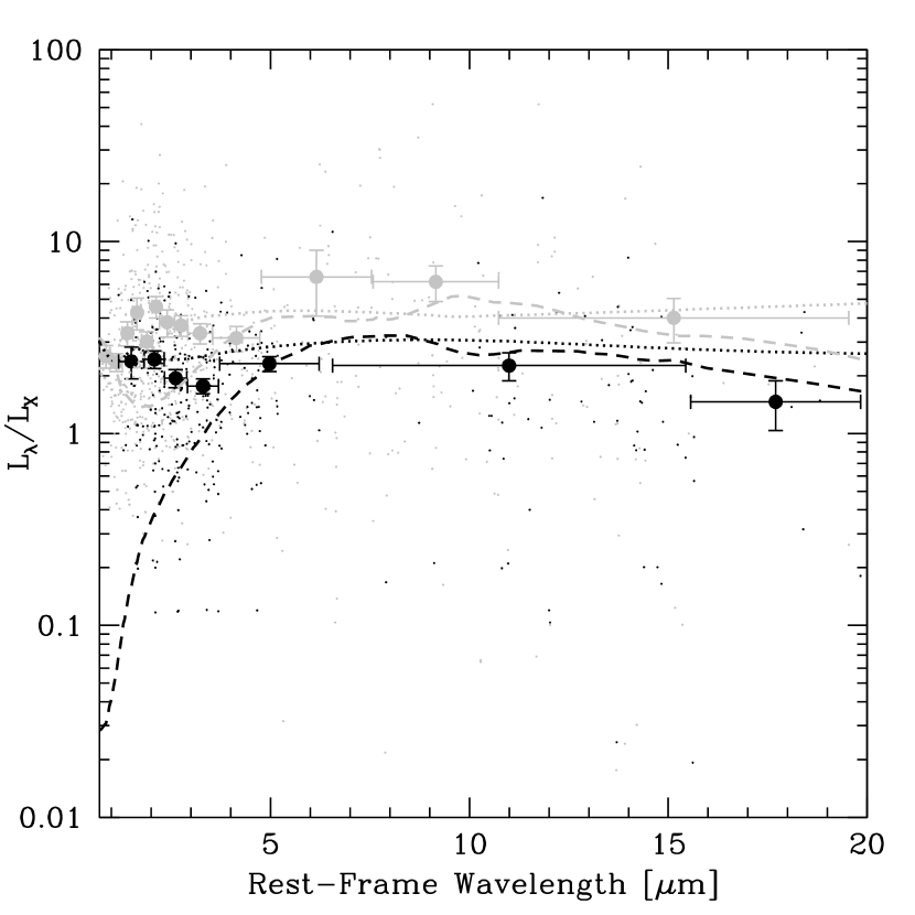
In order to compare with the observed averages for nearby Seyfert galaxies, in Figure 15 we also present the composite IR spectrum for local sources classified as Seyfert 1 (unobscured) and Seyfert 2 (obscured), as compiled by Polletta et al. (2007), normalized at a fiducial wavelength of 100 m, where the IR re-emission is expected to be fully isotropic. It is remarkable that both composite spectra agree well with our average values, thus indicating that the sources in our sample, most of them at =0.5-1 have very similar IR spectra to local active galaxies and higher luminosity sources. In addition, the results presented in Figure 15 allow to explain why Ramos Almeida et al. (2007) and Horst et al. (2008) reach apparently discrepant conclusions. While the work of Ramos Almeida et al. (2007) was based in observations at 6 m, where the contrast between obscured and unobscured sources is nearly maximal, Horst et al. (2008) used observations of a limited sample of sources at 12 m, where the contrast is smaller than at shorter wavelengths. Thus, it is possible that the results of Horst et al. (2008) are dominated by the intrinsic scatter in this relations, in particular given the low number of sources in their sample.
In Figure 15 we also compare the observed infrared luminosities with the predictions from torus models recently presented by Nenkova et al. (2008). These models assume a clumpy distribution for the obscuring material. While establishing the physical parameters of the dust surrounding the central region is a difficult task, which is beyond the scope of this paper, in Fig. 15 we show examples of the expected IR spectrum for obscured and unobscured sources. The assumed parameters are described by Nenkova et al. (2008) in the caption of their Figure 4, for a r-3 radial distribution of clouds. Following the basic assumption of the original AGN unification paradigm, the only difference between the obscured and unobscured model is the viewing angle. As can be seen, a decent agreement is found between the model spectrum and observations, in particular at wavelengths longer than 5 m. At shorter wavelengths, the additional contribution from the AGN host galaxy (not included in the model spectrum) starts to be significant, in particular for the obscured sources.
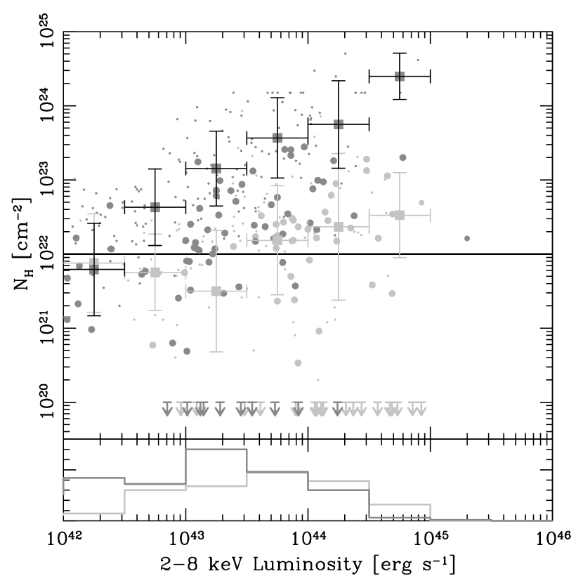
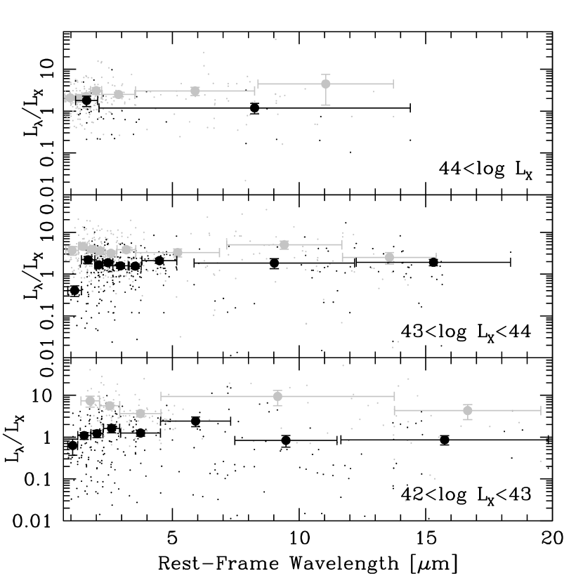
Taking advantage of the large number of sources in our sample, in Figure 16 we show / as a function of wavelength for sources separated in three luminosity bins: 1043 erg s-1, 1043 erg s-11044 erg s-1 and 1044 erg s-1. A clear conclusion from this figure is that the difference in the average ratio between obscured and unobscured sources is largest at the lowest luminosity bin, while for higher luminosity sources the / ratios become very similar. In their study of the mid-IR properties of nearby AGN, Polletta et al. (2007) found somewhat consistent results. According to their Figure 9, the ratio (at rest-frame 6 m) to for obscured sources, obtained combining their AGN2 and SF classes, is significantly lower than the ratio for unobscured AGN (their AGN1 class). In our interpretation of Figure 16, this increasing contrast for lower luminosity sources can be understood in terms of the luminosity dependence of the geometrical parameters of the absorbing region, in particular the opening angle, as described by Treister et al. (2008).
5. Conclusions
We presented here the first results from our optical spectroscopy program, aimed to provide identifications and redshifts for the X-ray sources detected by Chandra in the ECDF-S field. As part of this work we targeted 339 X-ray sources from the catalog of Virani et al. (2006) and obtained redshifts and identifications for 160 sources. We also added 26 sources with identifications obtained from the literature. While most of the sources with broad emission lines are found at 1, the mean redshift for the sources in our sample is 0.75. In order to separate obscured and unobscured AGN we adopted a mixed scheme, combining the optical spectroscopy information with the indication of the X-ray spectrum given by the hardness ratio. This hybrid scheme agrees very well in most cases with the amount of neutral Hydrogen column density measured in the X-ray spectrum for the brightest sources.
The optical colors of the obscured and/or low luminosity AGN are dominated by the host galaxy, and are on average redder than non-active galaxies, as was found previously by other authors. We also focused on the fraction of obscured AGN and its possible dependence on luminosity and redshift. For the latter, we confirmed at higher significance the results of Treister & Urry (2006), indicating that after correcting for selection effects the fraction of obscured AGN increases with redshift. Regarding a possible luminosity dependence, we confirmed the functional form derived by Treister & Urry (2005) and found that the population synthesis model of Gilli et al. (2007) significantly overestimates the fraction of obscured AGN at high luminosities. We also computed the AGN spatial density as a function of redshift and found results in agreement with the expected values using the luminosity function of Barger et al. (2005), but significant discrepancies with the luminosity functions of Ueda et al. (2003) and La Franca et al. (2005), which can however by most likely explained by the effects of incompleteness in our X-ray-selected sample.
Taking advantage of the deep multiwavelength data available in the ECDF-S we studied the infrared properties of the X-ray selected AGN with spectroscopic identifications. We found a significant difference in the fraction of bolometric light emitted at mid-IR wavelengths by obscured and unobscured AGN. These differences can be explained by the effects of dust self-absorption, for which the maximum contrast should be at 5-15 m. Furthermore, by separating our sample into luminosity bins we found that the contrast is larger for the lower luminosity sources. One possible interpretation for this result is that the opening angle is larger for high luminosity sources, such that the effects of self absorption are less important.
References
- Adami et al. (2005) Adami, C. et al. 2005, A&A, 443, 805
- Akylas & Georgantopoulos (2008) Akylas, A. & Georgantopoulos, I. 2008, A&A, 479, 735
- Akylas et al. (2006) Akylas, A., Georgantopoulos, I., Georgakakis, A., Kitsionas, S., & Hatziminaoglou, E. 2006, A&A, 459, 693
- Alonso-Herrero et al. (2008) Alonso-Herrero, A., Pérez-González, P. G., Rieke, G. H., Alexander, D. M., Rigby, J. R., Papovich, C., Donley, J. L., & Rigopoulou, D. 2008, ApJ, 677, 127
- Arnaud (1996) Arnaud, K. A. 1996, Astronomical Data Analysis Software and Systems V, 101, 17
- Baldry et al. (2004) Baldry, I. K., Glazebrook, K., Brinkmann, J., Ivezić, Ž., Lupton, R. H., Nichol, R. C., & Szalay, A. S. 2004, ApJ, 600, 681
- Ballantyne et al. (2006) Ballantyne, D. R., Everett, J. E., & Murray, N. 2006, ApJ, 639, 740
- Barger et al. (2003) Barger, A. J., Cowie, L. L., Capak, P., Alexander, D. M., Bauer, F. E., Fernandez, E., Brandt, W. N., Garmire, G. P., & Hornschemeier, A. E. 2003, AJ, 126, 632
- Barger et al. (2005) Barger, A. J., Cowie, L. L., Mushotzky, R. F., Yang, Y., Wang, W.-H., Steffen, A. T., & Capak, P. 2005, AJ, 129, 578
- Barvainis (1987) Barvainis, R. 1987, ApJ, 320, 537
- Bauer et al. (2004) Bauer, F. E., Alexander, D. M., Brandt, W. N., Schneider, D. P., Treister, E., Hornschemeier, A. E., & Garmire, G. P. 2004, AJ, 128, 2048
- Bell et al. (2004) Bell, E. F., Wolf, C., Meisenheimer, K., Rix, H.-W., Borch, A., Dye, S., Kleinheinrich, M., Wisotzki, L., & McIntosh, D. H. 2004, ApJ, 608, 752
- Brandt et al. (2001) Brandt, W. N., Alexander, D. M., Hornschemeier, A. E., Garmire, G. P., Schneider, D. P., Barger, A. J., Bauer, F. E., Broos, P. S., Cowie, L. L., Townsley, L. K., Burrows, D. N., Chartas, G., Feigelson, E. D., Griffiths, R. E., Nousek, J. A., & Sargent, W. L. W. 2001, AJ, 122, 2810
- Cardamone et al. (2007) Cardamone, C. N., Moran, E. C., & Kay, L. E. 2007, AJ, 134, 1263
- Cardamone et al. (2008) Cardamone, C. N., Urry, C. M., Damen, M., van Dokkum, P., Treister, E., Labbé, I., Virani, S. N., Lira, P., & Gawiser, E. 2008, ApJ, 680, 130
- Cirasuolo et al. (2007) Cirasuolo, M., McLure, R. J., Dunlop, J. S., Almaini, O., Foucaud, S., Smail, I., Sekiguchi, K., Simpson, C., Eales, S., Dye, S., Watson, M. G., Page, M. J., & Hirst, P. 2007, MNRAS, 380, 585
- Comastri et al. (1995) Comastri, A., Setti, G., Zamorani, G., & Hasinger, G. 1995, A&A, 296, 1
- Croom et al. (2001) Croom, S. M., Warren, S. J., & Glazebrook, K. 2001, MNRAS, 328, 150
- Davis et al. (2007) Davis, M. et al. 2007, ApJ, 660, L1
- De Luca & Molendi (2004) De Luca, A. & Molendi, S. 2004, A&A, 419, 837
- Della Ceca et al. (2008) Della Ceca, R., Caccianiga, A., Severgnini, P., Maccacaro, T., Brunner, H., Carrera, F. J., Cocchia, F., Mateos, S., Page, M. J., & Tedds, J. A. 2008, ArXiv e-prints, 805
- Fazio et al. (2004) Fazio, G. G. et al. 2004, ApJS, 154, 10
- Gawiser et al. (2006a) Gawiser, E. et al. 2006a, ApJS, 162, 1
- Gawiser et al. (2006b) —. 2006b, ApJ, 642, L13
- Georgakakis et al. (2008) Georgakakis, A., et al. 2008, MNRAS, 385, 2049
- Giacconi et al. (2001) Giacconi, R., Rosati, P., Tozzi, P., Nonino, M., Hasinger, G., Norman, C., Bergeron, J., Borgani, S., Gilli, R., Gilmozzi, R., & Zheng, W. 2001, ApJ, 551, 624
- Gilli et al. (2007) Gilli, R., Comastri, A., & Hasinger, G. 2007, A&A, 463, 79
- Gilli et al. (2005) Gilli, R., Daddi, E., Zamorani, G., Tozzi, P., Borgani, S., Bergeron, J., Giacconi, R., Hasinger, G., Mainieri, V., Norman, C., Rosati, P., Szokoly, G., & Zheng, W. 2005, A&A, 430, 811
- Gilli et al. (2001) Gilli, R., Salvati, M., & Hasinger, G. 2001, A&A, 366, 407
- Gilli et al. (2003) Gilli, R. et al. 2003, ApJ, 592, 721
- Gruber (1992) Gruber, D. E. 1992, in The X-ray Background, 44
- Hasinger et al. (2005) Hasinger, G., Miyaji, T., & Schmidt, M. 2005, A&A, 441, 417
- Hickox & Markevitch (2006) Hickox, R. C. & Markevitch, M. 2006, ApJ, 645, 95
- Hildebrandt et al. (2006) Hildebrandt, H., Erben, T., Dietrich, J. P., Cordes, O., Haberzettl, L., Hetterscheidt, M., Schirmer, M., Schmithuesen, O., Schneider, P., Simon, P., & Trachternach, C. 2006, A&A, 452, 1121
- Hönig & Beckert (2007) Hönig, S. F. & Beckert, T. 2007, MNRAS, 380, 1172
- Hönig et al. (2006) Hönig, S. F., Beckert, T., Ohnaka, K., & Weigelt, G. 2006, A&A, 452, 459
- Horst et al. (2008) Horst, H., Gandhi, P., Smette, A., & Duschl, W. J. 2008, A&A, 479, 389
- Horst et al. (2006) Horst, H., Smette, A., Gandhi, P., & Duschl, W. J. 2006, A&A, 457, L17
- Kalberla et al. (2005) Kalberla, P. M. W., Burton, W. B., Hartmann, D., Arnal, E. M., Bajaja, E., Morras, R., & Pöppel, W. G. L. 2005, A&A, 440, 775
- Krolik & Begelman (1988) Krolik, J. H. & Begelman, M. C. 1988, ApJ, 329, 702
- La Franca et al. (2005) La Franca, F. et al. 2005, ApJ, 635, 864
- La Franca & Cristiani (1997) La Franca, F., & Cristiani, S. 1997, AJ, 113, 1517
- Lawrence (1991) Lawrence, A. 1991, MNRAS, 252, 586
- Le Fèvre et al. (2004) Le Fèvre, O. et al. 2004, A&A, 428, 1043
- LeFevre et al. (2003) LeFevre, O. et al. 2003, in Presented at the Society of Photo-Optical Instrumentation Engineers (SPIE) Conference, Vol. 4841, Instrument Design and Performance for Optical/Infrared Ground-based Telescopes. Edited by Iye, Masanori; Moorwood, Alan F. M. Proceedings of the SPIE, Volume 4841, pp. 1670-1681 (2003)., ed. M. Iye & A. F. M. Moorwood, 1670–1681
- Lehmer et al. (2005) Lehmer, B. D. et al. 2005, ApJS, 161, 21
- Lira et al. (2002) Lira, P., Ward, M., Zezas, A., Alonso-Herrero, A., & Ueno, S. 2002, MNRAS, 330, 259
- Lutz et al. (2004) Lutz, D., Maiolino, R., Spoon, H. W. W., & Moorwood, A. F. M. 2004, A&A, 418, 465
- Makovoz & Marleau (2005) Makovoz, D. & Marleau, F. R. 2005, PASP, 117, 1113
- Mignano et al. (2007) Mignano, A., Miralles, J.-M., da Costa, L., Olsen, L. F., Prandoni, I., Arnouts, S., Benoist, C., Madejsky, R., Slijkhuis, R., & Zaggia, S. 2007, A&A, 462, 553
- Moran et al. (2002) Moran, E. C., Filippenko, A. V., & Chornock, R. 2002, ApJ, 579, L71
- Morrison & McCammon (1983) Morrison, R. & McCammon, D. 1983, ApJ, 270, 119
- Nandra et al. (2007) Nandra, K., Georgakakis, A., Willmer, C. N. A., Cooper, M. C., Croton, D. J., Davis, M., Faber, S. M., Koo, D. C., Laird, E. S., & Newman, J. A. 2007, ApJ, 660, L11
- Nandra et al. (1997) Nandra, K., George, I. M., Mushotzky, R. F., Turner, T. J., & Yaqoob, T. 1997, ApJ, 476, 70
- Nandra & Pounds (1994) Nandra, K. & Pounds, K. A. 1994, MNRAS, 268, 405
- Nenkova et al. (2008) Nenkova, M., Sirocky, M. M., Nikutta, R., Ivezić, Ž., & Elitzur, M. 2008, ApJ, 685, 160
- Nenkova et al. (2002) Nenkova, M., Ivezić, Ž., & Elitzur, M. 2002, ApJ, 570, L9
- Oke & Gunn (1983) Oke, J. B. & Gunn, J. E. 1983, ApJ, 266, 713
- Pier & Krolik (1992) Pier, E. A. & Krolik, J. H. 1992, ApJ, 401, 99
- Pier & Krolik (1993) —. 1993, ApJ, 418, 673
- Polletta et al. (2007) Polletta, M. et al. 2007, ApJ, 663, 81
- Ramos Almeida et al. (2007) Ramos Almeida, C., Pérez García, A. M., Acosta-Pulido, J. A., & Rodríguez Espinosa, J. M. 2007, AJ, 134, 2006
- Rieke et al. (2004) Rieke, G. H. et al. 2004, ApJS, 154, 25
- Risaliti et al. (1999) Risaliti, G., Maiolino, R., & Salvati, M. 1999, ApJ, 522, 157
- Rosati et al. (2002) Rosati, P. et al. 2002, ApJ, 566, 667
- Schawinski et al. (2008) Schawinski, K., Virani, S., Simmons, B., Urry, C.M., Treister, E. & Kaviraj, S. 2008, ApJ, submitted
- Schawinski et al. (2006) Schawinski, K. et al. 2006, Nature, 442, 888
- Schneider et al. (2002) Schneider, D. P. et al. 2002, AJ, 123, 567
- Scoville et al. (2007) Scoville, N. et al. 2007, ApJS, 172, 1
- Setti & Woltjer (1989) Setti, G. & Woltjer, L. 1989, A&A, 224, L21
- Silverman et al. (2008) Silverman, J. D. et al. 2008, ApJ, 675, 1025
- Simpson (2005) Simpson, C. 2005, MNRAS, 360, 565
- Spergel et al. (2007) Spergel, D. N. et al. 2007, ApJS, 170, 377
- Springel et al. (2005) Springel, V., Di Matteo, T., & Hernquist, L. 2005, MNRAS, 361, 776
- Steffen et al. (2003) Steffen, A. T., Barger, A. J., Cowie, L. L., Mushotzky, R. F., & Yang, Y. 2003, ApJ, 596, L23
- Szokoly et al. (2004) Szokoly, G. P. et al. 2004, ApJS, 155, 271
- Tozzi et al. (2006) Tozzi, P. et al. 2006, A&A, 451, 457
- Treister et al. (2005) Treister, E., Castander, F. J., Maccarone, T. J., Gawiser, E., Coppi, P. S., Urry, C. M., Maza, J., Herrera, D., Gonzalez, V., Montoya, C., & Pineda, P. 2005, ApJ, 621, 104
- Treister et al. (2007) Treister, E., Gawiser, E., van Dokkum, P., Lira, P., Urry, M., & The Musyc Collaboration. 2007, The Messenger, 129, 45
- Treister et al. (2008) Treister, E., Krolik, J. H., & Dullemond, C. 2008, ApJ, 679, 140
- Treister & Urry (2005) Treister, E. & Urry, C. M. 2005, ApJ, 630, 115
- Treister & Urry (2006) —. 2006, ApJ, 652, L79
- Treister et al. (2006) Treister, E., Urry, C. M., Van Duyne, J., Dickinson, M., Chary, R.-R., Alexander, D. M., Bauer, F., Natarajan, P., Lira, P., & Grogin, N. A. 2006, ApJ, 640, 603
- Treister et al. (2004) Treister, E. et al. 2004, ApJ, 616, 123
- Ueda et al. (2003) Ueda, Y., Akiyama, M., Ohta, K., & Miyaji, T. 2003, ApJ, 598, 886
- Vanzella et al. (2005) Vanzella, E. et al. 2005, A&A, 434, 53
- Vanzella et al. (2006) —. 2006, A&A, 454, 423
- Vanzella et al. (2008) —. 2008, A&A, 478, 83
- Virani et al. (2006) Virani, S. N., Treister, E., Urry, C. M., & Gawiser, E. 2006, AJ, 131, 2373
- Weiner et al. (2005) Weiner, B. J. et al. 2005, ApJ, 620, 595
- Wolf et al. (2004) Wolf, C. et al. 2004, A&A, 421, 913
- Zheng et al. (2004) Zheng, W. et al. 2004, ApJS, 155, 73
| Run | Instrument | Masks | Slit Width | Avg. Seeing | Total Sources | X-ray Sources | EfficiencyaaDefined as the fraction of X-ray sources identified. |
|---|---|---|---|---|---|---|---|
| 26-27/10/2003 | IMACS | 4 | 1.0′′ | 1′′ | 291 | 74 | 57% |
| 4-7/2/2005 | IMACS | 2 | 1.2′′ | 0.8′′ | 180 | 64 | 57% |
| 2-3/11/2005 | IMACS | 2 | 1.2′′ | 0.6′′ | 194 | 29 | 66% |
| 25-27/10/2006 | IMACS | 3 | 1.0′′ | 0.5-1.5′′ | 280 | 143 | 32% |
| 21-22/11/2006 | IMACS | 1 | 1.2′′ | 0.8′′ | 109 | 17 | 20% |
| 18-20/2/2007bbThe mask from the Nov. 2006 run was re-observed in order to obtain 5 hours of integration time. | IMACS | 1 | 1.2′′ | 1′′ | 109 | 17 | 20% |
| Period 78 | VIMOS | 4 | 1.0′′ | 1′′ | 283 | 96 | 54% |
| IDaaX-ray ID number from the catalog of Virani et al. (2006) | X-ray Flux (erg cm2s-1) | Hardness Ratio | Redshift | Instrument | Class.ddUNK: Unkown, OAGN: Obscured AGN, UAGN: Unobuscred AGN, ELG: Emission line galaxy, ALG: Absorption line galaxy, STAR: star. | log (X-ray Lum.) | 24 m (mJy) | |||||||||
|---|---|---|---|---|---|---|---|---|---|---|---|---|---|---|---|---|
| Softbb0.5–2 keV | Hardcc2–8 keV | Value | Upper | Lower | (erg s-1) | Flux | Error | SourceeeSurvey in which the 24 m source is identified. F: FIDEL, G: GOODS. | Value | Upper | Lower | (cm-2) | ||||
| 2 | 2.040e-15 | 4.690e-15 | 1.000 | 0.000 | 0.000 | 9.990ffA =9.990 corresponds to a targeted source for which the redshift could not be measured. | IMACS | UNK | —— | 51.27 | 1.42 | F | —– | —– | —– | —— |
| 3 | 2.670e-15 | 6.620e-15 | -1.000 | 0.000 | 0.000 | 9.990 | IMACS | UNK | —— | 223.50 | 1.33 | F | 1.900 | —– | —– | 20.843 |
| 4 | 3.650e-14 | 6.590e-14 | -0.354 | 0.030 | 0.031 | 2.011 | IMACS | OAGN | 45.273 | 229.90 | 1.60 | F | 1.836 | 0.123 | 0.117 | 20.941 |
| 6 | 6.760e-15 | 8.590e-15 | -0.498 | 0.069 | 0.075 | 3.031 | VIMOS | UAGN | 44.821 | 482.20 | 1.22 | F | 2.045 | 0.402 | 0.347 | 21.087 |
| 7 | 1.260e-15 | 4.300e-15 | -0.054 | 0.126 | 0.146 | 0.289 | IMACS | ELG | 42.044 | 92.09 | 1.26 | F | —– | —– | —– | —— |
Note. — This table is published in its entirety in the electronic edition of the Astrophysical Journal. A portion is shown here for guidance regarding its form and content.