Study of $D^{0}\to\pi^{-}e^{+}\nu_{e}$, $D^{+}\to\pi^{0}e^{+}\nu_{e}$, $D^{0}\to K^{-}e^{+}\nu_{e}$, and $D^{+}\to\bar{K}^{0}e^{+}\nu_{e}$ in Tagged Decays of the $\psi(3770)$ Resonance

Abstract

Using $\psi(3770)\rightarrow D\bar{D}$ events collected with the CLEO-c detector at the Cornell $e^{+}e^{-}$ storage ring, tagged by fully reconstructing one $D$ meson in a hadronic decay mode, we measure absolute branching fractions and differential decay rates for $D^{0}\rightarrow\pi^{-}e^{+}\nu_{e}$, $D^{+}\rightarrow\pi^{0}e^{+}\nu_{e}$, $D^{0}\rightarrow K^{-}e^{+}\nu_{e}$, and $D^{+}\rightarrow\bar{K}^{0}e^{+}\nu_{e}$. The measured decay rates are used to study semileptonic form factors governing these transitions and to test unquenched Lattice QCD (LQCD) calculations. We average our results with previously published CLEO-c measurements of the same quantities using a neutrino reconstruction technique. Combining LQCD calculations of form factor absolute normalizations $f_{+}(0)$ and measurements of $f^{\pi}_{+}(0)|V_{cd}|$ and $f^{K}_{+}(0)|V_{cs}|$, we find $|V_{cd}|=0.222(8)(3)(23)$ and $|V_{cs}|=1.018(10)(8)(106)$, where the uncertainties are statistical, experimental systematic, and from LQCD, respectively.

I Introduction

The quark mixing parameters are fundamental constants of the Standard Model of particle physics. They determine the nine weak-current quark coupling elements of the Cabibbo-Kobayashi-Maskawa (CKM) matrix ckm . In the Standard Model the CKM matrix is unitary. Measuring the quark couplings tests the unitarity of the matrix.

The extraction of the quark couplings is difficult because quarks are bound inside hadrons by the strong interaction. Semileptonic decays are the preferred way to determine the CKM matrix elements as the strong interaction binding effects are confined to the hadronic current. They are parameterized by form factors that are calculable, for example, by lattice quantum chromodynamics (LQCD) and QCD sum rules. Nevertheless, form factor uncertainties dominate the precision with which the CKM matrix elements can be determined VubVcb .

Studies of the semileptonic decays of $D$ mesons play an important role in understanding the CKM matrix. First these decays allow the robust determination of the couplings $|V_{cs}|$ and $|V_{cd}|$ by combining measured branching fractions with form factor calculations. Second $|V_{cs}|$ and $|V_{cd}|$ are tightly constrained when the CKM matrix is assumed to be unitary. Therefore measurements of charm semileptonic decay rates, when combined with the values of $|V_{cs}|$ and $|V_{cd}|$ constrained by the unitarity of the CKM matrix, rigorously test theoretical predictions of $D$ meson semileptonic form factors.

Recently using $\psi(3770)\rightarrow D\bar{D}$ events and a neutrino reconstruction technique combined with an independent measurement of the number of $D$ mesons, CLEO reported the most precise determinations of the absolute branching fractions and differential decay rates $d\Gamma/dq^{2}$ for the decays $D^{0}\to\pi^{-}e^{+}\nu_{e}$, $D^{+}\to\pi^{0}e^{+}\nu_{e}$, $D^{0}\to K^{-}e^{+}\nu_{e}$, and $D^{+}\to\bar{K}^{0}e^{+}\nu_{e}$ Nadia . (Throughout this paper charge-conjugate modes are implied.) The differential decay rates were used to determine the absolute magnitude and shape of the semileptonic form factors and to determine $|V_{cs}|$ and $|V_{cd}|$. In this paper we present a complementary analysis which measures the same quantities with similar precision in a common data set but with a different technique that is independent of the number of $D$ mesons in the data sample. The two analyses obtain consistent results, providing increased confidence in their correctness, and each represents a marked improvement in our understanding of charm semileptonic decays.

As the two analyses use a common data set, the results are correlated. We calculate average values of the branching fractions, form factors and $|V_{cs}|$ and $|V_{cd}|$ measured in the two analyses, taking into account correlations between them. The average values represent the best determinations of these quantities with the CLEO-c 281 pb^-1 data set.

The paper is organized as follows. We review the semileptonic decay formalism in Sec. II. The data sample and CLEO-c detector are described in Sec. III. The analysis technique to identify semileptonic decays is introduced in Sec. IV. In Secs. V and VI we describe the use of this technique to measure the absolute branching fractions, differential decay rates and form factor parameters for $D^{0}$ ($D^{+}$) decays to $\pi^{-}e^{+}\nu_{e}$ ($\pi^{0}e^{+}\nu_{e}$) and $K^{-}e^{+}\nu_{e}$ ($\bar{K}^{0}e^{+}\nu_{e}$). The extraction of CKM parameters is described in Sec. VII. In Sec. VIII we average the results presented here with the results obtained in Nadia . Finally, in Sec. IX a summary is provided.

II Semileptonic Decay Formalism

The matrix element for a semileptonic decay $M_{i}(q_{i}\bar{q}^{\prime})\rightarrow M_{f}(q_{f}\bar{q}^{\prime})\ell^{+}\nu_{\ell}$ where $M_{i}$ and $M_{f}$ are the initial and final state mesons, $q_{i}$ and $q_{f}$ are the initial and final state quarks, and $\bar{q}^{\prime}$ is a spectator anti-quark, can be written as

$$\mathcal{M}(M_{i}\rightarrow M_{f}\ell^{+}\nu_{\ell})=-i\frac{G_{F}}{\sqrt{2}}V_{q_{i}q_{f}}^{*}L^{\mu}H_{\mu},$$

where $G_{F}$ is the Fermi constant, $V_{q_{i}q_{f}}$ is the appropriate CKM matrix element, and $L^{\mu}$ and $H_{\mu}$ are the leptonic and hadronic currents, respectively. The leptonic current is known and can be written in terms of the lepton and neutrino Dirac spinors, $u_{\ell}$ and $v_{\nu}$,

$$L^{\mu}=\bar{u}_{\ell}\gamma^{\mu}(1-\gamma_{5})v_{\nu}.$$

The underlying simplicity of the weak transition $q_{i}\rightarrow q_{f}W^{+}$ is obscured by the strong interaction as the initial and final state quarks are bound within hadrons. The hadronic current can be written as

$$H_{\mu}=\langle M_{f}|\bar{q}_{f}\gamma_{\mu}(1-\gamma_{5})q_{i}|M_{i}\rangle.$$

The hadronic current describes the non-perturbative strong interaction physics of hadron formation. Usually, one exploits the fact that the hadronic current transforms as a four vector under Lorentz transformations by parameterizing it with a set of invariant form factors. This is achieved by constructing all possible quantities with transformation properties of four vectors from the momenta of particles involved in the decay, their spin - polarization vectors and invariant tensors, and expanding the hadronic current in terms of these with an invariant form factor multiplying each of them. The form factors can only be functions of Lorentz scalars. In $M_{i}\rightarrow M_{f}\ell^{+}\nu_{\ell}$, there is one such invariant, which is usually chosen to be $q^{2}$, the square of the invariant mass of the virtual $W$.

In pseudoscalar-to-pseudoscalar semileptonic decays ($P_{i}(q_{i}\bar{q})\rightarrow P_{f}(q_{f}\bar{q})\ell^{+}\nu_{\ell}$), the hadronic current has a simple structure:

$$\langle P_{f}(p_{f})|V^{\mu}|P_{i}(p_{i})\rangle$$

$$\quad=f_{+}(q^{2})\left((p_{i}+p_{f})^{\mu}-\frac{m_{i}^{2}-m_{f}^{2}}{q^{2}}(p_{i}-p_{f})^{\mu}\right)$$

$$\qquad+f_{0}(q^{2})\frac{m_{i}^{2}-m_{f}^{2}}{q^{2}}(p_{i}-p_{f})^{\mu},$$ (1)

where $p_{i}$ ($m_{i}$) and $p_{f}$ ($m_{f}$) are the four-momenta (masses) of the initial $P_{i}$ and final $P_{f}$ mesons, and $f_{+}(q^{2})$ and $f_{0}(q^{2})$ are the form factors governing the transition. Kinematic constraints require $f_{+}(0)=f_{0}(0)$. In the limit of negligible lepton mass, which is applicable for $\ell=e$, only one form factor remains,

$$\langle P_{f}(p_{f})|V^{\mu}|P_{i}(p_{i})\rangle=f_{+}(q^{2})(p_{i}+p_{f})^{\mu}.$$

The form factor $f_{+}(q^{2})$ measures the probability to form the final state hadron; it is largest when the daughter meson is stationary in the parent meson rest frame $q^{2}=q^{2}_{\rm max}$, and smallest when the daughter meson is moving with maximum velocity in the parent meson rest frame $q^{2}=0$.

The differential decay rate is given by

$$\frac{d\Gamma}{dq^{2}}=\frac{G^{2}_{F}|V_{q_{i}q_{f}}|^{2}p^{3}_{P_{f}}}{24\pi^{3}}|f_{+}(q^{2})|^{2},$$ (2)

where $p_{P_{f}}$ is the magnitude of the three-momentum of the $P_{f}$ meson in the rest frame of $P_{i}$. The shape of the $q^{2}$ distribution is dominated by the dependence on $p^{3}_{P_{f}}$, which arises because the decay proceeds via a $P$-wave. This dependence significantly enhances the rate at low $q^{2}$. We perform fits to the differential decay rate to measure the four semileptonic modes $D\rightarrow Ke^{+}\nu$ and $D\rightarrow\pi e^{+}\nu$. In this paper we denote the form factor governing $D\rightarrow Ke^{+}\nu$ and $D\rightarrow\pi e^{+}\nu$ by $f_{+}^{K}(q^{2})$ and $f_{+}^{\pi}(q^{2})$, respectively.

II.1 Parametrization of the Form Factor $q^{2}$ Dependence

The dependence of the form factors on $q^{2}$ is unknown, as it is determined by non-perturbative QCD. One may express the form factors in terms of a dispersion relation, an approach that has been well established in the literature (see, for example, Ref. BSW and references therein):

$$f_{+}\left(q^{2}\right)=\frac{f_{+}\left(0\right)}{1-\lambda}\frac{1}{1-\frac{\textstyle q^{2}}{\textstyle M^{2}_{\rm pole}}}+\frac{1}{\pi}\int_{(m_{D}+m_{P})^{2}}^{\infty}{\frac{{\rm Im}(f_{+}\left(t\right))}{t-q^{2}-i\varepsilon}dt}.$$ (3)

where $M_{\rm pole}$ is the mass of the lowest lying $(q_{i}\bar{q}_{f})$ meson with the appropriate quantum numbers: for $D\rightarrow Ke^{+}\nu_{e}$ it is $D_{s}^{\ast+}(1^{-})$ and for $D\rightarrow\pi e^{+}\nu_{e}$ it is $D^{*+}(1^{-})$, the parameter $\lambda$ gives the contribution from the vector pole at $q^{2}=0$, $m_{D}$ is the mass of the $D$ meson, and $m_{P}$ is the mass of the final state pseudoscalar meson. It is common to write the dispersive representation in terms of an explicit pole and a sum of effective poles,

$$f_{+}(q^{2})=\frac{\textstyle f_{+}(0)}{\textstyle 1-\lambda}\frac{\textstyle 1}{\textstyle 1-\frac{\textstyle q^{2}}{\textstyle M^{2}_{\rm pole}}}+\sum_{k=1}^{N}\frac{\textstyle\rho_{k}}{\textstyle 1-\frac{\textstyle q^{2}}{\textstyle\gamma_{k}M^{2}_{\rm pole}}},$$ (4)

where $\rho_{k}$ and $\gamma_{k}$ are expansion parameters that are not predicted.

A series expansion around $q^{2}=t_{0}$  Boyd ; Boyd-2 ; Arnesen ; rhill , where $t_{0}$ is defined below, is commensurate with the dispersion relations. As expansions in $q^{2}$ suffer from convergence problems due to the presence of nearby poles, the expansion is formulated as an analytic continuation into the $t=q^{2}$ complex plane. There is a branch cut on the real axis for $t>M_{K,\pi}^{2}$ corresponding to $D(K,\pi)$ production, that is mapped onto the unit circle by the variable $z$ defined as

$$z(q^{2},t_{0}) = \frac{\sqrt{t_{+}-q^{2}}-\sqrt{t_{+}-t_{0}}}{\sqrt{t_{+}-q^{2}}+\sqrt{t_{+}-t_{0}}},$$

$$t_{\pm} = \left(m_{D}\pm m_{P}\right)^{2},$$ (5)

where $t_{0}$ is the arbitrary $q^{2}$ value that maps to $z=0$. We choose $t_{0}=t_{+}(1-\sqrt{1-t_{-}/t_{+}})$ because this choice minimizes the maximum value of $z$ in the decay ($|z_{{\rm max}}|=0.051{\rm~{}for~{}}D\rightarrow Ke^{+}\nu_{e}{\rm~{}and~{}}|z_{{\rm max}}|=0.17{\rm~{}for~{}}D\rightarrow\pi e^{+}\nu_{e}$).

The form factor is given by

$$f_{+}(q^{2})=\frac{a_{0}}{P(q^{2})\phi(q^{2},t_{0})}\left(1+\sum_{k=1}^{\infty}a_{k}(t_{0})z(q^{2},t^{0})^{k}\right),$$ (6)

where $P(q^{2})=1$ for $D\rightarrow\pi$ and $P(q^{2})=z(q^{2},m_{D_{s}^{*+}}^{2})$ for $(D\rightarrow K)$, and $\phi$ is arbitrary. Physically $P$ accounts for the presence of the pole, and $\phi$ is chosen to enable a simple expression for the series in terms of the $a_{k}$. We follow Ref. rhill :

$$\phi(q^{2},t_{0}) = c\left(\frac{z(q^{2},0)}{-q^{2}}\right)^{5/2}\left(\frac{z(q^{2},t_{0})}{t_{0}-q^{2}}\right)^{-1/2}\times$$ (7)

$$\left(\frac{z(q^{2},t_{-})}{t_{-}-q^{2}}\right)^{-3/4}\frac{t_{+}-q^{2}}{(t_{+}-t_{0})^{1/4}}.$$

This choice leads to the constraint

$$\sum_{k=1}^{n_{c}}a_{k}^{2}\leq 1$$ (8)

for any choice of $n_{c}$. To leading order the coefficient $c$ is given by

$$c=\sqrt{\pi m_{c}^{2}/3},$$ (9)

where $m_{c}$ is the charm quark mass, which we take to be 1.2 GeV/c². An advantage of the $z$ expansion is that it is model independent and satisfies analyticity and unitarity. In addition, measuring the $a_{i}$ in $D\rightarrow\pi\ell^{+}\nu_{\ell}$ constrains the class of form factors needed to fit $B\rightarrow\pi\ell^{+}\nu_{\ell}$ and hence may improve the determination of $|V_{ub}|$. Finally, in Heavy Quark Effective Theory (HQET) HQET there exist relations between the $a_{i}$ in $D$ and $B$ semileptonic decays.

The expansion parameters are not predicted. As $z$ is small, the series is expected to converge quickly. Recently BABAR BABAR-06 , using a data sample of 75,000 $D^{0}\to K^{-}e^{+}\nu_{e}$ events, found the differential rate to be well described with only a linear term. In this work we will fit the data to both linear and quadratic terms and use the series expansion for our main results. There are alternatives to the $z$ expansion mere-q2-expansion .

In order to compare to lattice QCD calculations and previous measurements, we will also compare the data to other parametrizations of the form factor $q^{2}$ dependence. A variety of models have been traditionally used to parameterize the $q^{2}$ dependence. The most common, based on vector meson dominance BSW , uses only the first term in the dispersion relation. In this “simple pole model” the $q^{2}$ dependence is given by

$$f_{+}(q^{2})=\frac{\textstyle f_{+}(0)}{\textstyle(1-\frac{\textstyle q^{2}}{\textstyle M_{\rm pole}^{2}})}.$$ (10)

Previous measurements of the $q^{2}$ spectrum in $D^{0}\rightarrow K^{-}\ell^{+}\nu_{\ell}$, the best measured charm semileptonic decay, find a value of the pole mass many standard deviations from $M_{D_{s}^{*}}$  Nadia ; BABAR-06 ; CLEOIII ; FOCUS-05 ; BELLE-06 . At low to medium values of $q^{2}$ the $q^{2}$ spectrum is distorted compared to a simple pole, suggesting contributions from a spectrum of poles above the pole with the lowest mass.

The modified pole or Becirevic-Kaidalov (BK) parametrization modpole attempts to address the shortcoming of the simple pole model by keeping the first term in the dispersion relation sum. The form factor is given by

$$f_{+}(q^{2})=\frac{\textstyle f_{+}(0)}{\textstyle(1-\frac{\textstyle q^{2}}{\textstyle M_{\rm pole}^{2}})(1-\alpha\frac{\textstyle q^{2}}{\textstyle M_{\rm pole}^{2}})},$$ (11)

where $M_{\rm pole}$ is the spectroscopic pole mass and $\alpha$, a free parameter, is an additional “effective” pole which represents the total contribution of all additional poles.

In current data the $q^{2}$ evolution of form factors are indistinguishable from straight lines. Therefore it is convenient to define the physical shape observables in terms of form factor slopes at $t=0$ Hill05 ; Hill06FPCP

$${1\over\beta} \equiv {m_{D}^{2}-m_{P}^{2}\over f_{+}(0)}\left.df_{0}\over dt\right|_{t=0}$$

$$\delta \equiv 1-{m_{D}^{2}-m_{P}^{2}\over f_{+}(0)}\left(\left.df_{+}\over dt\right|_{t=0}-\left.df_{0}\over dt\right|_{t=0}\right).$$ (12)

The quantities $\beta$ and $\delta$ depend on the masses of the mesons involved, and as they are physical quantities they are independent of the renormalization scale or scheme.

The BK parametrization requires several assumptions to reduce the multiple parameters initially present (Eq. (4)) to one. Specifically, it is assumed that $\beta$, which measures scaling violations, is near unity, and $\delta$, which measures spectator quark interactions, is near zero. This sets the physical observable

$$1+1/\beta-\delta=\frac{m_{D}^{2}-m_{P}^{2}}{f_{+}(0)}\frac{df_{+}}{dq^{2}}\sim 2~{}({\rm at~{}}q^{2}=0),$$ (13)

as noted in Ref. Hill06FPCP , corresponding to $\alpha\sim 1.75$ for $D\to K\ell^{+}\nu_{\ell}$ and 1.34 for $D\to\pi\ell^{+}\nu_{\ell}$. Previous experimental measurements of the $q^{2}$ spectrum in $D\rightarrow K/\pi\ell^{+}\nu_{\ell}$ do not agree with this value of $\alpha$ Nadia ; BABAR-06 ; CLEOIII ; FOCUS-05 ; BELLE-06 .

Although the simple pole model and modified pole model are unable to describe the $q^{2}$ spectrum of the data when the pole mass is fixed to the relevant spectroscopic pole, or $\alpha\sim 1.75$ for $D\to K\ell^{+}\nu_{\ell}$ and 1.34 for $D\to\pi\ell^{+}\nu_{\ell}$, they do describe the data well for values of the shape parameters many standard deviations from the expected values.

II.2 Form Factor Calculations

A variety of model dependent calculations of form factors exist. In these models the form factors are evaluated at a fixed value of $q^{2}$, e.g., $q^{2}~{}=~{}0$ or $q^{2}~{}=~{}q^{2}_{{\rm max}}=(m_{D}-m_{P})^{2}$, and are extrapolated over the full range of $q^{2}$ using a parametrization, such as those discussed above.

Quark model calculations estimate meson wave functions and use them to compute the matrix elements that appear in the hadronic current. There are a large variety of theoretical calculations survey-of-models . Among them the ISGW model ISGW has been widely used to simulate heavy hadron semileptonic decays. This model is expected to be valid in the vicinity of $q^{2}=q^{2}_{\rm max}$, the region of maximum overlap between the initial and final meson wave functions.

In the ISGW model the form factors are assumed to have the form

$$f(q^{2})=f(q^{2}_{\rm max})e^{-a(q^{2}_{\rm max}-q^{2})}.$$ (14)

The ISGW2 model ISGW2 , an update of the ISGW model, incorporates constraints from heavy quark symmetry. It uses a dipole term for the form factor $q^{2}$ dependence expressed in terms of the radius of a meson ($r$) rather than the mass of the appropriate $(q_{i}\bar{q}_{f})$ meson:

$$f_{+}(q^{2})=f_{+}(q^{2}_{\rm max})\left(1+\frac{r^{2}}{12}\left(q_{\rm max}^{2}-q^{2}\right)\right)^{-2}.$$ (15)

The ISGW2 model predicts $f_{+}^{K}(q^{2}_{\rm max})=1.23$ and $r^{K}=1.12{\rm~{}GeV}^{-1}$ ISGW2 . Previous measurements (e.g., Refs. CLEOIII ; FOCUS-05 ; BELLE-06 ; BABAR-06 ) do not agree with these values.

QCD sum rules QCD-sum-rules-1 ; QCD-sum-rules-2 , are expected to be valid at low $q^{2}$. For $D^{0}\rightarrow K^{-}\ell^{+}\nu_{\ell}$, and using a value of 150 MeV for the strange quark mass, one obtains QCD-sum-rules-2 $f^{K}_{+}(0)=0.78(11)$ and $\alpha_{K}=0.07^{+0.15}_{-0.07}$ using the modified pole ansatz. For $D\rightarrow\pi\ell^{+}\nu_{\ell}$ QCD-sum-rules-2 reports $f^{\pi}_{+}(0)=0.65(11)$ and $\alpha_{\pi}=0.01^{+0.11}_{-0.07}$.

The above models are based on theoretical assumptions and, in consequence, introduce a difficult to quantify theoretical uncertainty that is significantly larger than the presently achievable experimental statistical and systematic uncertainties combined. Therefore this limits the precision with which $|V_{cs}|$ and $|V_{cd}|$ can be determined from exclusive semileptonic charm meson decays.

Lattice QCD computes $f_{+}(q^{2})$ from first principles. Current results must be extrapolated to physical values of light quark masses and corrected for finite lattice size and discretization effects. There have been several evaluations of $f_{+}(q^{2})$ for different values of the momentum transfer in the quenched approximation Flynn ; Abada . These results, which do not include QCD vacuum polarization, have been combined Flynn , to give $f_{+}^{K}(0)=0.73(7)$. LQCD calculations which incorporate QCD vacuum polarization (unquenched calculations) have produced results that agree with experiment to within a few percent for a number of quantities Davies . The first unquenched LQCD calculation unquenched_LQCD of form factors in $D\rightarrow Ke^{+}\nu_{e}$ and $D\rightarrow\pi e^{+}\nu_{e}$ reports $f_{+}^{K}(0)=0.73(3)(7)$, $\alpha_{K}=0.50(4)$, $f_{+}^{\pi}(0)=0.64(3)(6)$, and $\alpha_{\pi}=0.44(4)$ using the modified pole ansatz to parameterize the $q^{2}$ dependence of the form factor. Here the systematic uncertainty is dominated by the effect of discretization. While the form factors are currently calculated to a modest precision of ten percent, the uncertainties are systematically improvable to a precision that matches, or exceeds, the experimental measurements presented here and in Nadia . Accordingly, we use unquenched_LQCD to extract values for $|V_{cs}|$ and $|V_{cd}|$ in this work.

III Data Sample and the CLEO-c Detector

The data sample used in this analysis consists of 281 pb^-1 of $e^{+}e^{-}$ annihilation data taken at the $\psi(3770)$, which is about 40 MeV above the $D\bar{D}$ pair production threshold. (Throughout this paper $D$ is used to denote $D^{0}$ and $D^{+}$.) The data include approximately $1.0\times 10^{6}$ $D^{0}\bar{D}^{0}$ events and $0.8\times 10^{6}$ $D^{+}D^{-}$ events.

CLEO-c is a general-purpose solenoidal detector. The charged particle tracking system covers a solid angle of 93% of $4\pi$ and consists of a small-radius six-layer low mass stereo wire drift chamber concentric with and surrounded by a 47-layer cylindrical drift chamber. The chambers operate in a 1.0 T magnetic field and achieve a momentum resolution of $\sim$0.6% at $p=$1 GeV/$c$. The main drift chamber provides specific-ionization ($dE/dx$) measurements that discriminate between charged pions and kaons. Additional hadron identification is provided by a Ring-Imaging Cherenkov (RICH) detector covering approximately 80% of $4\pi$. Identification of positrons and detection of neutral pions rely on an electromagnetic calorimeter consisting of 7800 cesium iodide crystals and covering 95% of $4\pi$. The calorimeter achieves a photon energy resolution of 2.2% at $E_{\gamma}=$1 GeV and 5% at 100 MeV. The CLEO-c detector is described in detail elsewhere cleo_detector .

The response of the CLEO-c detector was studied using a GEANT-based GEANT Monte Carlo (MC) simulation. To develop selection criteria and test the analysis technique several MC simulations are used. $\psi(3770)\rightarrow D\bar{D}$ events are generated using EvtGen EvtGen and each $D$ meson is allowed to decay in accordance with the best experimental and theoretical information. We refer to this as “generic MC”. The MC sample generated corresponds to an integrated luminosity of about $11~{}\rm{fb^{-1}}$ which is a factor 40 larger than the data. Semileptonic signal decays are generated with the modified pole model form factors modpole with parameters from the most recent unquenched LQCD calculations unquenched_LQCD .

Due to the tagging technique employed in the analysis, backgrounds from the non-$D\bar{D}$ processes $e^{+}e^{-}\rightarrow q\bar{q}$, where $q$ is a $u$, $d$, or $s$ quark, $e^{+}e^{-}\rightarrow\tau^{+}\tau^{-}$, and $e^{+}e^{-}\rightarrow\psi(2S)\gamma$, are nearly absent. These non-$D\bar{D}$ processes are also modeled using MC simulation and are scaled absolutely according to their measured cross sections at the $\psi(3770)$.

A second type of MC sample, which we refer to as “signal MC”, consists of several samples of $\psi(3770)\rightarrow D\bar{D}$ events in which the $\bar{D}$ is allowed to decay to all possible final states, and the $D$ decays to a specific semileptonic final state.

IV Event Reconstruction

The reconstruction technique used in this analysis was first applied by the Mark III collaboration MkIII at SPEAR. This technique was used to measure $D$ semileptonic branching fractions with a smaller data sample at CLEO-c DSemilBFs-2005 . That data sample was too small to study charm semileptonic form factors, which are the focus of studies reported in this paper.

The presence of two $D$ mesons in a $\psi(3770)$ event allows a tag sample to be defined in which a $\bar{D}$ is reconstructed in a hadronic decay mode. A sub-sample is then defined in which a positron and a set of hadrons, as a signature of a semileptonic decay, are required in addition to the tag. Tagging a $\bar{D}$ meson in a $\psi(3770)$ decay provides a $D$ with known four-momentum, allowing a semileptonic decay to be reconstructed with no kinematic ambiguity, even though the neutrino is undetected.

The tag yield can be expressed as $N_{{\rm tag}}=2N_{DD}{\cal B}_{{\rm tag}}\epsilon_{{\rm tag}}$, where $N_{DD}$ is the produced number of $D\bar{D}$ pairs, ${\cal{B}}_{{\rm tag}}$ is the branching fraction of hadronic modes used in the tag sample, and $\epsilon_{{\rm tag}}$ is the tag efficiency. The yield of tags with a semileptonic decay can be expressed as $N_{{\rm tag,SL}}=2N_{DD}{\cal{B}}_{{\rm tag}}{\cal{B}}_{{\rm SL}}\epsilon_{{\rm tag,SL}}$ where ${\cal{B}}_{{\rm SL}}$ is the semileptonic decay branching fraction, including subsidiary branching fractions, and $\epsilon_{{\rm tag,SL}}$ is the efficiency of finding the tag and the semileptonic decay in the same event. From the expressions for $N_{{\rm tag}}$ and $N_{{\rm tag,SL}}$ we obtain

$${\cal{B}}_{{\rm SL}}=\frac{N_{\rm tag,SL}}{N_{\rm tag}}\frac{\epsilon_{\rm tag}}{\epsilon_{\rm tag,SL}}=\frac{N_{\rm tag,SL}/\epsilon}{N_{\rm tag}},$$ (16)

where $\epsilon=\epsilon_{\rm tag,SL}/\epsilon_{\rm tag}$ is the effective signal efficiency. The branching fraction determined by tagging is an absolute measurement. It is independent of the integrated luminosity and number of $D$ mesons in the data sample. Due to the large solid angle acceptance and high segmentation of the CLEO-c detector and the low multiplicity of the events $\epsilon_{\rm tag,SL}\approx\epsilon_{\rm tag}\epsilon_{\rm SL}$, where $\epsilon_{\rm SL}$ is the semileptonic decay efficiency. Hence the ratio $\epsilon_{\rm tag,SL}/\epsilon_{\rm tag}$ is insensitive to most systematic effects associated with the tag mode and the absolute branching fraction determined with this procedure is nearly independent of the tag mode. Below, we first describe the procedure used for the reconstruction of tags followed by that for the reconstruction of semileptonic decays DSemilBFs-2005 .

IV.1 Tag Selection

Hadronic tracks must have momenta above 50 MeV/$c$ and $|\cos{\theta}|<0.93$, where $\theta$ is the angle between the track direction and the beam axis. Identification of hadrons is based on measurements of specific ionization in the main drift chamber and information from the RICH. Pion and kaon candidates are required to have $dE/dx$ measurements within three standard deviations (3$\sigma$) of the expected value. For tracks with momenta greater than 700 MeV/$c$, RICH information, if available, is combined with $dE/dx$. The efficiencies ($95$% or higher) and misidentification rates (a few percent) are determined with charged pion and kaon samples from hadronic $D$ decays.

We select $\pi^{0}$ candidates from pairs of photons, each having an energy of at least 30 MeV, and a shower shape consistent with that expected for a photon. A kinematic fit is performed constraining the invariant mass of the photon pair to the known $\pi^{0}$ mass. The candidate is accepted if the unconstrained invariant mass is within 3$\sigma$, where $\sigma$ (typically 6 MeV/$c^{2}$) is determined for that candidate from the kinematic fit, and the kinematic parameters for the $\pi^{0}$ determined with the fit are used in further reconstruction.

Candidate events are selected by reconstructing a $\bar{D}^{0}$ or $D^{-}$ tag in the following hadronic final states: $K^{+}\pi^{-}$, $K^{+}\pi^{-}\pi^{0}$, $K^{+}\pi^{-}\pi^{0}\pi^{0}$, $K^{+}\pi^{-}\pi^{-}\pi^{+}$, $K_{S}^{0}\pi^{0}$, $K_{S}^{0}\pi^{-}\pi^{+}$, $K_{S}^{0}\pi^{-}\pi^{+}\pi^{0}$, and $K^{-}K^{+}$ for neutral tags, and $K^{0}_{S}\pi^{-}$, $K^{+}\pi^{-}\pi^{-}$, $K^{0}_{S}\pi^{-}\pi^{0}$, $K^{+}\pi^{-}\pi^{-}\pi^{0}$, $K^{0}_{S}\pi^{-}\pi^{-}\pi^{+}$, and $K^{-}K^{+}\pi^{-}$ for charged tags. These modes constitute about 46% and 28% of all $\bar{D}^{0}$ and $D^{-}$ decays, respectively. Tagged events are selected using two variables: $\Delta E\equiv E_{D}-E_{\rm beam}$, the difference between the energy of the tag candidate ($E_{D}$) and the beam energy ($E_{\rm beam}$), and the beam-constrained mass $M_{\rm bc}\equiv\sqrt{E_{\rm beam}^{2}/c^{4}-|\vec{p}_{D}|^{2}/c^{2}}$, where $\vec{p}_{D}$ is the measured momentum of the tag candidate. Note that the use of $E_{\rm beam}$ instead of $E_{D}$ improves the resolution of $M_{\rm bc}$ by one order of magnitude, to about $2~{}{\rm MeV/c^{2}}$, which is dominated by the beam energy spread. If multiple candidates are present in the same tag mode, the one candidate per tag flavor with the smallest $\Delta E$ is chosen.

The number of tags reconstructed in each mode is obtained by imposing a mode dependent requirement on $\Delta E$, counting the number of events in the signal region of $M_{\rm bc}$, defined as $-6.5~{}{\rm MeV}/c^{2}<(M_{\rm bc}-m_{D})<9.5~{}{\rm MeV}/c^{2}$, where $m_{D}$ PDG2004 is the known $D$ meson mass, and subtracting the background contribution from it. Fits to the $M_{\rm bc}$ distributions, shown in Figs. 1 and 2, are made using the procedure described in cleoc-Dtagging . We fit the $M_{\rm bc}$ distributions to a signal shape and one or more background components. The signal shape includes the effects of beam energy smearing, initial state radiation, the line shape of the $\psi(3770)$, and reconstruction resolution. The background is described by an ARGUS function ARGUS , which models combinatorial contributions. The background contribution in the signal region is estimated by integrating this function. The yields of the eight neutral tag modes and the six charged tag modes, and their reconstruction efficiencies as determined with the generic MC simulation, are given in Tables 1 and 2. There are approximately $3.1\times 10^{5}$ and $1.6\times 10^{5}$ neutral and charged tags, respectively.

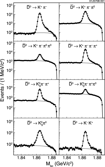
Figure 1: Fits (solid line) to the $M_{\rm bc}$ distributions in data for eight $\bar{D}^{0}$ tag modes. The backgrounds are shown by the dashed line.

Figure 2: Fits (solid line) to the $M_{\rm bc}$ distributions in data for six $D^{-}$ tag modes. The backgrounds are shown by the dashed line.

Table 1: Yields with statistical uncertainties and reconstruction efficiencies of $\bar{D}^{0}$ tags.

Tag Mode	$N_{\rm tag}$	$\epsilon_{\rm tag}$ (%)
$\bar{D}^{0}\to K^{+}\pi^{-}$	$51002(230)$	$64.77(3)$
$\bar{D}^{0}\to K^{+}\pi^{-}\pi^{0}$	$98117(347)$	$33.30(1)$
$\bar{D}^{0}\to K^{+}\pi^{-}\pi^{0}\pi^{0}$	$23040(220)$	$14.41(1)$
$\bar{D}^{0}\to K^{+}\pi^{-}\pi^{-}\pi^{+}$	$77641(303)$	$45.46(2)$
$\bar{D}^{0}\to K^{0}_{S}\pi^{-}\pi^{+}$	$24533(187)$	$38.33(2)$
$\bar{D}^{0}\to K^{0}_{S}\pi^{-}\pi^{+}\pi^{0}$	$20355(260)$	$17.81(5)$
$\bar{D}^{0}\to K^{0}_{S}\pi^{0}$	$8175(99)$	$31.01(5)$
$\bar{D}^{0}\to K^{-}K^{+}$	$4614(76)$	$57.35(9)$
All Neutral Tags	$307478(657)$

Table 2: Yields with statistical uncertainties and reconstruction efficiencies of $D^{-}$ tags .

Tag Mode	$N_{\rm tag}$	$\epsilon_{\rm tag}$ (%)
$D^{-}\to K^{+}\pi^{-}\pi^{-}$	$79896(291)$	$53.81(2)$
$D^{-}\to K^{+}\pi^{-}\pi^{-}\pi^{0}$	$23740(196)$	$25.23(2)$
$D^{-}\to K^{0}_{S}\pi^{-}$	$11456(113)$	$45.14(5)$
$D^{-}\to K^{0}_{S}\pi^{-}\pi^{0}$	$25159(210)$	$21.97(2)$
$D^{-}\to K^{0}_{S}\pi^{-}\pi^{-}\pi^{+}$	$16431(191)$	$31.58(3)$
$D^{-}\to K^{-}K^{+}\pi^{-}$	$6794(100)$	$44.72(5)$
All Charged Tags	$163476(477)$

IV.2 Selection of Semileptonic Decays

After a tag is identified, we search for a positron and a set of hadrons recoiling against the tag. (Muons are not used as $D$ semileptonic decays at the $\psi(3770)$ produce low momentum leptons for which the CLEO-c muon identification is not efficient.) Positron candidates are required to have momenta of at least 200 MeV/$c$ and to satisfy $|\cos{\theta}|$ $<$ 0.90, where $\theta$ is the angle between the positron direction and the beam axis. The efficiency for positron identification rises from about $50\%$ at 200 MeV/$c$ to 95% just above 300 MeV/$c$ and is roughly constant thereafter. The rate for misidentifying charged pions and kaons as positrons averaged over the momentum range is approximately 0.1%. The energy lost by positrons to bremsstrahlung photons is partially recovered by adding showers that are within $5^{\circ}$ of the positron momentum and are not matched to other particles. The selection of $\pi^{-}$, $\pi^{0}$, $K^{-}$, and $K^{0}_{S}$ candidates is identical to that used for tags.

The tag and the semileptonic candidate are then combined. Events that include tracks other than those of the tag and the semileptonic candidate are vetoed extra_track_cut . After all selection criteria are applied, multiple candidates in the same event are rare in all modes except $D^{+}\to\pi^{0}e^{+}\nu_{e}$. For $D^{+}\to\pi^{0}e^{+}\nu_{e}$, in the few percent of events with multiple candidates, one combination is chosen per tag candidate based on the proximity of the invariant masses of the $\pi^{0}$ candidates to the expected mass.

Semileptonic decays are identified using the variable $U\equiv E_{\rm miss}-c|\vec{p}_{\rm miss}|$, where $E_{\rm miss}$ and $\vec{p}_{\rm miss}$ are the missing energy and momentum of the $D$ meson decaying semileptonically, calculated using the difference of the four-momentum of the tag and that of the observed products of the semileptonic decay. If the decay products of the semileptonic decay have been correctly identified, $U$ is expected to be zero, since only a neutrino is undetected. To improve the resolution in $U$, the crossing angle of the beams ($\sim 3$ mrad) is allowed for by recalculating all track momenta and shower energies in the $\psi(3770)$ rest frame, and the four-momentum of the tag is approximated by ($E_{\rm beam}/c,\sqrt{(E_{\rm beam}/c)^{2}-(cm_{D})^{2}}\hat{p}_{D}$), where $\hat{p}_{D}$ is the unit direction vector of the $D$ in the $\psi(3770)$ rest frame determined using the direction of the $\bar{D}$ tag in the same frame. Due to the finite resolution of the detector, the distribution in $U$ is approximately Gaussian, centered at $U=0$ with $\sigma\sim 12~{}{\rm MeV}$, for all modes except $D^{+}\to\pi^{0}e^{+}\nu_{e}$, for which $\sigma$ is approximately two times larger.

Using this procedure we obtain the $U$ distributions shown in Fig. 3. For each mode a clear signal is evident centered on $U=0$, while backgrounds are very small near $U=0$. In $D^{0}\rightarrow\pi^{-}e^{+}\nu_{e}$ the peak at positive $U$ is from two sources: $D^{0}\rightarrow K^{-}e^{+}\nu_{e}$ when a $K^{-}$ is misidentified as a $\pi^{-}$ (peak at 130 MeV) and from $D\rightarrow K^{-}\pi^{+}\pi^{0}$ where the $K^{-}$ is mistaken for an electron and the $\pi^{0}$ is unobserved (peak at 180 MeV). This background is present because each event is not required to have both a $D^{0}$ and a $\bar{D}^{0}$. Specifically, on the semileptonic side of the event both $D^{0}\rightarrow\pi^{-}e^{+}\nu_{e}$ and $\bar{D}^{0}\rightarrow\pi^{+}e^{-}\bar{\nu}_{e}$ are accepted, on the tag side for example both $\bar{D}^{0}\rightarrow K^{+}\pi^{-}$ and $D^{0}\rightarrow K^{-}\pi^{+}$ are accepted. The kaon produced in the decay of the tag is not required to have the same charge as the lepton produced in the semileptonic decay. If this requirement were made the $D\rightarrow K^{-}\pi^{+}\pi^{0}$ background would be removed, but decay sequences where the tag undergoes a doubly Cabibbo suppressed decay such as $D^{0}\rightarrow K^{+}\pi^{-},$ and $\bar{D}^{0}\rightarrow\pi^{+}e^{-}\bar{\nu}_{e}$ would be removed as well.

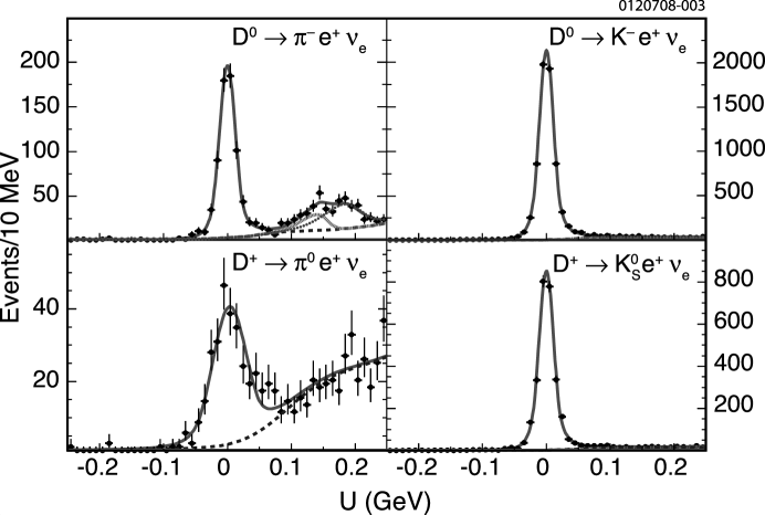
Figure 3: Fits (solid line) to the $U$ distributions in data (points) for $D^{0}\to\pi^{-}e^{+}\nu_{e}$, $D^{0}\to K^{-}e^{+}\nu_{e}$, $D^{+}\to\pi^{0}e^{+}\nu_{e}$, and $D^{+}\to K^{0}_{S}e^{+}\nu_{e}$. The background contributions are represented by dotted or dashed lines. In $D^{0}\to\pi^{-}e^{+}\nu_{e}$ the background peaks at positive $U$ are described in the text.

The yield for each semileptonic mode is determined from a fit to the corresponding $U$ distribution, as shown in Fig. 3 with all tag modes combined. The yields are reported in Table 3. In each case the signal function consists of a Gaussian to describe the core of the $U$ distribution and two power law tails to account for initial and final state radiation (ISR and FSR):

$$f=\left\{\begin{array}[]{lr}a_{1}(\frac{n_{1}}{\alpha_{1}}-\alpha_{1}+t)^{-n_{1}}&t>\alpha_{1}\\[4.0pt] e^{-\frac{t^{2}}{2}}&-\alpha_{2}<t<\alpha_{1}\\[4.0pt] a_{2}(\frac{n_{2}}{\alpha_{2}}-\alpha_{2}-t)^{-n_{2}}&t<-\alpha_{2}\end{array}\right.,$$ (17)

where $t\equiv(U-U_{\rm mean})/\sigma_{U}$, $a_{1}\equiv\left(n_{1}/\alpha_{1}\right)^{n_{1}}e^{-{\alpha_{1}^{2}}/{2}}$, and $a_{2}\equiv\left(n_{2}/\alpha_{2}\right)^{n_{2}}e^{-{\alpha_{2}^{2}}/{2}}$. The parameters describing the tails of the signal function ($\alpha_{1}$, $\alpha_{2}$, $n_{1}$, and $n_{2}$) are always fixed in fits to the data to the values found in signal MC simulation. The $\sigma_{U}$ is fixed to the value predicted by the MC simulation in the fit for $D^{0}\rightarrow\pi^{0}e^{+}\nu_{e}$, which has the smallest signal yield and the largest background level among the four semileptonic modes, and allowed to float in the fits for the other modes.

The background functions are determined from the generic MC simulation. The backgrounds are small and arise mostly from misreconstructed semileptonic decays with correctly reconstructed tags. The background shape parameters are fixed, while the background normalizations are allowed to float in all fits to the data.

V Absolute Branching Fraction Measurements

V.1 Determination of the Branching Fractions

The absolute semileptonic branching fractions are obtained from our tagged semileptonic yields $N_{\rm tag,SL}$, tag yields $N_{\rm tag}$, and the efficiencies $\epsilon$, using Eq. (16). The simulation of each semileptonic mode employs the simple pole model with $M_{\text{pole}}=2.0~{}{\rm GeV/c^{2}}$. The efficiency depends weakly on $M_{\text{pole}}$; accordingly the efficiencies are re-weighted to the value of $M_{\rm pole}$ measured in the data. These efficiencies are then weighted by the tag yields shown in Tables 1 and 2 to obtain the overall efficiency. The absolute semileptonic branching fractions are obtained using these weighted efficiencies. Table 3 presents our absolute semileptonic branching fraction measurements with statistical and systematic uncertainties. A description of how the systematic uncertainties are obtained is provided in the next subsection.

The procedure for measuring semileptonic branching fractions is tested using the generic MC sample. In the test, the MC sample is treated identically to the data. In addition, the procedure was separately tested for each combination of tag and semileptonic mode. We find that the input and output branching fractions are consistent within statistical uncertainties in all cases. The largest deviation is observed for $D^{+}\to\bar{K}^{0}e^{+}\nu_{e}$ with all tag modes combined, where the discrepancy is less than one third of the statistical uncertainty on the measurement.

To check the consistency of the measurement of the semileptonic branching fractions, we have also measured semileptonic branching fractions for each tag mode separately for the two Cabibbo allowed final states where there are adequate statistics in each tag mode. We present the results in Tables 4 and 5.

We note that the effective semileptonic efficiency is larger for tag modes with higher multiplicity. This happens primarily because tag reconstruction efficiencies in events with the second $D$ meson decaying hadronically are slightly smaller compared to signal events with the second $D$ meson decaying to a low multiplicity semileptonic final state.

We find that the branching fractions are consistent among tag modes. The results in Tables 4 and 5 also demonstrate consistency between the weighted averages of the individual tag mode branching fractions and the branching fractions obtained with all tag modes combined.

Table 3: Signal efficiencies, yields, and branching fractions in this work (first four columns) and, for comparison, the branching fractions measured using the first 56 pb^-1 CLEO-c $\psi(3770)$ data sample  DSemilBFs-2005 , and values from PDG-04 PDG2004 . The first uncertainty is statistical and the second systematic in the fourth and fifth columns, and statistical or total in the other columns.

Decay Mode	$\epsilon$ (%)	$N_{\rm tag,SL}$	$\mathcal{B}_{\rm SL}$ (%)	$\mathcal{B}_{\rm SL}$ (%) (56 pb-1)	$\mathcal{B}_{\rm SL}$ (%) (PDG-04)
$D^{0}\rightarrow\pi^{-}e^{+}\nu_{e}$	$72.54(11)$	$699(28)$	$0.314(13)(4)$	$0.262(25)(8)$	$0.36(6)$
$D^{+}\rightarrow\pi^{0}e^{+}\nu_{e}$	$44.72(13)$	$281(19)$	$0.384(27)(23)$	$0.44(6)(3)$	$0.31(15)$
$D^{0}\rightarrow K^{-}e^{+}\nu_{e}$	$61.06(7)$	$6786(84)$	$3.61(5)(5)$	$3.44(10)(10)$	$3.58(18)$
$D^{+}\rightarrow\bar{K}^{0}e^{+}\nu_{e}$	$20.01(4)$	$2910(55)$	$8.90(17)(21)$	$8.71(38)(37)$	$6.7(9)$

Table 4: $D^{0}\to K^{-}e^{+}\nu_{e}$ semileptonic yields in data, the semileptonic efficiency for each hadronic tag mode, $\epsilon$, and the branching fraction measurement for each hadronic tag mode. The last two lines show the weighted average of the individual measurements and the result from the fit with all tag modes combined.

Mode	$N_{\rm tag,SL}$	$\epsilon$ (%)	$\mathcal{B}_{\rm SL}$ (%)
$K^{+}\pi^{-}$	$1088(34)$	$59.36(15)$	$3.60(11)$
$K^{+}\pi^{-}\pi^{0}$	$2143(47)$	$61.66(12)$	$3.55(8)$
$K^{+}\pi^{-}\pi^{0}\pi^{0}$	$593(25)$	$67.11(30)$	$3.84(15)$
$K^{+}\pi^{-}\pi^{-}\pi^{+}$	$1693(42)$	$59.44(13)$	$3.67(9)$
$K^{0}_{S}\pi^{-}\pi^{+}$	$516(23)$	$59.47(24)$	$3.54(16)$
$K^{0}_{S}\pi^{-}\pi^{+}\pi^{0}$	$474(22)$	$64.46(30)$	$3.61(17)$
$K^{0}_{S}\pi^{0}$	$160(13)$	$60.52(43)$	$3.23(26)$
$K^{-}K^{+}$	$118(11)$	$59.45(51)$	$4.32(42)$
Average:			$3.61(5)$
Combined Fit:	$6786(84)$	$61.06(7)$	$3.61(5)$

Table 5: $D^{+}\to\bar{K}^{0}e^{+}\nu_{e}$ semileptonic yields in data, the semileptonic efficiency for each hadronic tag mode, $\epsilon$, and the branching fraction measurement for each hadronic tag mode. The semileptonic efficiency includes subsidiary branching fractions subsidiarybf . The last two lines show the weighted average of the individual measurements and the result from the fit with all tag modes combined.

Mode	$N_{\rm tag,SL}$	$\epsilon$ (%)	$\mathcal{B}_{\rm SL}$ (%)
$K^{+}\pi^{-}\pi^{-}$	$1437(39)$	$19.88(5)$	$9.04(25)$
$K^{+}\pi^{-}\pi^{-}\pi^{0}$	$430(21)$	$20.51(9)$	$8.83(44)$
$K^{0}_{S}\pi^{-}$	$201(14)$	$19.91(18)$	$8.81(46)$
$K^{0}_{S}\pi^{-}\pi^{0}$	$443(22)$	$20.17(9)$	$8.73(43)$
$K^{0}_{S}\pi^{-}\pi^{-}\pi^{+}$	$272(17)$	$19.82(11)$	$8.35(53)$
$K^{-}K^{+}\pi^{-}$	$130(12)$	$19.97(16)$	$9.59(88)$
Average :			$8.89(17)$
Combined Fit:	$2910(55)$	$20.01(4)$	$8.90(17)$

V.2 Study of Systematic Uncertainties for Absolute Branching Fractions

We have considered the following sources of systematic uncertainty in the measurements of branching fractions and give our estimates of their magnitudes in parentheses. The uncertainties associated with the efficiency for finding a track (0.3% for each pion, kaon, or positron, combined in quadrature with an additional 0.6% for each kaon), for reconstructing a $\pi^{0}$ (4.3%), and for reconstructing a $K_{S}^{0}$ (1.8%), are estimated using missing mass techniques described in cleoc-Dtagging . The uncertainty in the positron identification efficiency (1.0%) is obtained using a comparison of the detector response to positrons from radiative processes in the data and MC simulation. The effect of the event complexity is incorporated by studying positrons both in isolation and embedded in hadronic events. Uncertainties in the charged pion and kaon identification efficiencies (0.1% per pion and 0.2% per kaon) are estimated using hadronic $D$ meson decays. The uncertainty in the number of tags (0.4%) is estimated by using alternative signal functions in the fits to the $M_{\rm bc}$ distributions and by varying the end point of the background function ARGUS . The uncertainty associated with the requirement that there be no additional tracks in tagged semileptonic events (0.3%) is estimated by comparing fully reconstructed $D\bar{D}$ events in data and MC simulation. The uncertainty associated with the number of signal events is estimated by using an alternative signal function (a double Gaussian) in the fits and by counting events in the signal region (4.2% for $D^{+}\to\pi^{0}e^{+}\nu_{e}$, 0.3% for all other modes). The uncertainty in the semileptonic reconstruction efficiencies due to imperfect knowledge of the semileptonic form factors (0.0% to 0.3% depending on mode) is estimated by varying the form factor shape parameters in the MC simulation within uncertainties in their measurements reported in Sec. VI.4. The uncertainty associated with the simulation of FSR and bremsstrahlung radiation in the detector material (0.4%) is estimated by varying the amount of FSR modeled by the PHOTOS algorithm PHOTOS and by repeating the analysis without recovery of photons radiated by the positron and comparing to the standard results. The uncertainty associated with the simulation of ISR ($e^{+}e^{-}\rightarrow D\bar{D}\gamma$) is negligible. There is a systematic uncertainty due to finite MC statistics (0.1% to 0.3% depending on mode).

Table 6: Summary of systematic uncertainties considered in the measurements of absolute branching fractions of the four semileptonic modes. The modes are labeled by their final state hadrons.

		Systematic uncertainty (%)
Source		$K^{-}$	$\pi^{-}$	$K_{S}^{0}$	$\pi^{0}$
Number of $D$ tags		0.4	0.4	0.4	0.4
Electron ID efficiency		1.0	1.0	1.0	1.0
Hadron ID efficiency		0.2	0.1	0.0	0.0
Track finding efficiency		0.8	0.6	0.9	0.3
$\pi^{0}$ finding efficiency		0.0	0.0	0.0	4.3
$K^{0}_{S}$ finding efficiency		0.0	0.0	1.8	0.0
Unused tracks		0.3	0.3	0.3	0.3
Signal shape fit function		0.3	0.3	0.3	4.2
Simulation of FSR		0.4	0.4	0.4	0.4
Simulation of form factors		0.0	0.1	0.1	0.3
Limited MC statistics		0.1	0.2	0.2	0.3
Total uncertainty		1.5	1.4	2.4	6.1

Table 6 is a summary of the systematic uncertainties associated with the measurement of the four absolute semileptonic branching fractions. These estimates of systematic uncertainty are added in quadrature to obtain the total systematic uncertainty: 1.4%, 6.1%, 1.5%, and 2.4% for $D^{0}\to\pi^{-}e^{+}\nu_{e}$, $D^{+}\to\pi^{0}e^{+}\nu_{e}$, $D^{0}\to K^{-}e^{+}\nu_{e}$, and $D^{+}\to\bar{K}^{0}e^{+}\nu_{e}$, respectively.

V.3 Comparison to Previous Measurements

The branching fraction measurements with all tag modes combined for each of the four semileptonic modes reported in Table 3, are in good agreement with previous CLEO-c measurements using the same technique DSemilBFs-2005 obtained with a smaller data sample, and supersede them. In Table 3 we also compare our measurements to PDG 2004 PDG2004 averages. We compare to PDG 2004 because subsequent PDG averages PDG2006 ; PDG2008 are dominated by our previous CLEO-c measurements. In Table 7 we compare our measurements of ${\cal B}(D^{0}\rightarrow K^{-}e^{+}\nu_{e})$ and ${\cal B}(D^{0}\rightarrow\pi^{-}e^{+}\nu_{e})$ to previous measurements and to theoretical predictions. Our measurements agree well with previous measurements including the CLEO-c neutrino reconstruction analysis Nadia , which we denote by “untagged” hereinafter.

Table 7: Comparison of ${\cal B}(D^{0}\rightarrow K^{-}\ell^{+}\nu_{\ell})$ and ${\cal B}(D^{0}\rightarrow\pi^{-}\ell^{+}\nu_{\ell})$ values among different experiments and theoretical predictions. The first uncertainty is statistical, the second is systematic. The third uncertainty in the BABAR measurement is from the normalization to ${\cal B}(D^{0}\rightarrow K^{-}\pi^{+})$.

	$K^{-}\ell^{+}\nu_{\ell}(\%)$	$\pi^{-}\ell^{+}\nu_{\ell}$ (0.1%)
PDG (2004) PDG2004	3.58(18)	3.6(6)
BES II ($e$) BESII	3.82(40)(27)	3.3(13)(3)
LQCD unquenched_LQCD	3.77(29)(74)	3.16(25)(70)
LQCD (Abada) Abada	2.99(45)	2.4(6)
QCD SR (Ball) QCD-sum-rules-1	2.7(6)	1.6(3)
LCSR (KRWWY) QCD-sum-rules-2	3.6(14)	2.7(10)
LCSR (WWZ) WWZ	3.9(1.2)	3.0(9)
CLEO-c ($e$) DSemilBFs-2005	3.44(10)(10)	2.62(25)(8)
Belle ($e,\mu$) BELLE-06	3.45(7)(20)	2.55(19)(16)
BABAR ($e$) BABAR-06	3.522(27)(45)(65)	–
CLEO-c (tagged, $e$)	3.61(5)(5)	3.14(13)(4)
CLEO-c (untagged, $e$) Nadia	3.56(3)(9)	2.99(11)(9)

The widths of the isospin conjugate exclusive semileptonic decay modes of the $D^{0}$ and $D^{+}$ are related by isospin invariance of the hadronic current. The ratio $\Gamma(D^{0}\rightarrow K^{-}e^{+}\nu_{e})/\Gamma(D^{+}\rightarrow\bar{K}^{0}e^{+}\nu_{e})$ is expected to be unity, while the corresponding ratio for pions is expected to be two. Using our results and the lifetimes $\tau_{D^{0}}=410.3(1.5)\times 10^{-15}{\rm s}$and $\tau_{D^{+}}=1040(7)\times 10^{-15}{\rm s}$ PDG2004 , we obtain

$$\frac{\Gamma(D^{0}\rightarrow K^{-}e^{+}\nu_{e})}{\Gamma(D^{+}\rightarrow\bar{K}^{0}e^{+}\nu_{e})}=1.03(2)(2)$$ (18)

and

$$\frac{\Gamma(D^{0}\rightarrow\pi^{-}e^{+}\nu_{e})}{2\Gamma(D^{+}\rightarrow\pi^{0}e^{+}\nu_{e})}=1.04(9)(6),$$ (19)

where correlated and uncorrelated systematic uncertainties are taken into account. These ratios are consistent with isospin predictions, and supersede the corresponding ratios in Ref. DSemilBFs-2005 , which were measured with the same technique. These ratios are also consistent with the CLEO-c untagged analysis Nadia , and two less precise results: a measurement from BES II using the same technique BESII_ratio and an indirect measurement from FOCUS FOCUS_ratio .

As the data are consistent with isospin invariance, the precision of each branching fraction can be improved by averaging the $D^{0}$ and $D^{+}$ results for isospin conjugate pairs. For the isospin-averaged semileptonic decay widths, with correlations among systematic uncertainties taken into account, we find

$$\Gamma(D\rightarrow Ke^{+}\nu_{e})=8.73(9)(15)\times 10^{-2}{\rm ps^{-1}}$$ (20)

and

$$\Gamma(D\rightarrow\pi e^{+}\nu_{e})=0.76(3)(2)\times 10^{-2}{\rm ps^{-1}},$$ (21)

where for the latter partial width we have used $\Gamma(D^{0}\rightarrow\pi^{-}e^{+}\nu_{e})=2\Gamma(D^{+}\rightarrow\pi^{0}e^{+}\nu_{e})$. The measured ratio of decay widths for $D\rightarrow\pi e^{+}\nu_{e}$ and $D\rightarrow Ke^{+}\nu_{e}$ provides a test of the LQCD charm semileptonic rate ratio prediction unquenched_LQCD . Using the results obtained in this analysis, we find

$$\frac{\Gamma(D^{0}\rightarrow\pi^{-}e^{+}\nu_{e})}{\Gamma(D^{0}\rightarrow K^{-}e^{+}\nu_{e})}=0.0868(38)(4)$$ (22)

and

$$\frac{2\Gamma(D^{+}\rightarrow\pi^{0}e^{+}\nu_{e})}{\Gamma(D^{+}\rightarrow\bar{K}^{0}e^{+}\nu_{e})}=0.0863(64)(53).$$ (23)

These results are consistent with LQCD unquenched_LQCD and with previous measurements Nadia ; CLEOIII ; pikenu_focus . Finally, by averaging the $D^{0}$ and $D^{+}$ results for isospin conjugate pairs we obtain

$$\frac{\Gamma(D\rightarrow\pi e^{+}\nu_{e})}{\Gamma(D\rightarrow Ke^{+}\nu_{e})}=0.0868(33)(14),$$ (24)

where we have again used $\Gamma(D^{0}\rightarrow\pi^{-}e^{+}\nu_{e})=2\Gamma(D^{+}\rightarrow\pi^{0}e^{+}\nu_{e})$. A complete set of ratios of partial semileptonic decay widths measured in this analysis is given in Table  8.

Table 8: Ratios of semileptonic decay widths of $D^{0}$ and $D^{+}$ to the pseudoscalar mesons $\pi$ and $K$ (first four lines) and the isospin averaged ratio of semileptonic decay widths (fifth line). The uncertainties are statistical and systematic.

Ratios	Measured values
$\Gamma(D^{0}\to K^{-}e^{+}\nu_{e})/\Gamma(D^{+}\to\bar{K}^{0}e^{+}\nu_{e})$	$1.030(24)(20)$
$\Gamma(D^{0}\to\pi^{-}e^{+}\nu_{e})/2\Gamma(D^{+}\to\pi^{0}e^{+}\nu_{e})$	$1.037(86)(57)$
$\Gamma(D^{0}\to\pi^{-}e^{+}\nu_{e})/\Gamma(D^{0}\to K^{-}e^{+}\nu_{e})$	$0.0868(38)(4)$
$2\Gamma(D^{+}\to\pi^{0}e^{+}\nu_{e})/\Gamma(D^{+}\to\bar{K}^{0}e^{+}\nu_{e})$	$0.0863(64)(53)$
$\Gamma(D\to\pi e^{+}\nu_{e})/\Gamma(D\to Ke^{+}\nu_{e})$	$0.0868(33)(14)$

VI Study of Semileptonic Differential Decay Rates

VI.1 Measurement of the Differential Decay Rate

We now describe how the efficiency-corrected absolutely-normalized differential decay rate distributions are obtained. Full event reconstruction allows a direct measurement of the neutrino momentum with excellent resolution. The invariant mass squared of the $e^{+}\nu_{e}$ pair, $q^{2}$, is calculated in the $\psi(3770)$ rest frame in the following way (using as an example $D^{0}\to K^{-}e^{+}\nu_{e}$):

$$q^{2}=(E_{\rm beam}-E_{K})^{2}-(-\vec{p}_{\rm tag}-\vec{p}_{K})^{2},$$ (25)

$$\vec{p}_{\rm tag}=\hat{p}_{\rm tag}\sqrt{E_{\rm beam}^{2}-m_{D}^{2}},$$ (26)

where $E_{K}$ and $\vec{p}_{K}$ are the energy and three-momentum of the kaon. The $q^{2}$ resolutions ($q^{2}_{\rm reconstructed}-q^{2}_{\rm generated}$) averaged over the entire $q^{2}$ range are about 0.012 (GeV$/c^{2})^{2}$ for $D^{0}\to\pi^{-}e^{+}\nu_{e}$, $D^{0}\to K^{-}e^{+}\nu_{e}$ and $D^{+}\to\bar{K}^{0}e^{+}\nu_{e}$, and approximately 0.040 (GeV$/c^{2})^{2}$ for $D^{+}\to\pi^{0}e^{+}\nu_{e}$. For $D^{+}\to\pi^{0}e^{+}\nu_{e}$, the $q^{2}_{\rm reconstructed}-q^{2}_{\rm generated}$ distribution is well described by a Gaussian. For other semileptonic modes these distributions are consistent with a double Gaussian with $\sigma$’s that differ by a factor of 2.5, with the wider Gaussian mostly due to FSR.

As the $D$ mesons are produced almost at rest at the $\psi(3770)$, and the CLEO-c detector is nearly hermetic, the semileptonic reconstruction efficiencies are almost constant across the $q^{2}$ range. In consequence the shape of the $q^{2}$ spectrum receives only minor distortions due to detector acceptance. The excellent $q^{2}$ resolution likewise leads to only minor distortions due to $q^{2}$ smearing.

Events satisfying the reconstruction criteria of Sec. IV that lie in the $U$ signal region, defined as $-60\;{\rm MeV}\leq U\leq 60\;{\rm MeV}$, are sorted into bins of $q^{2}$. Ten bins of equal size ($q^{2}_{\rm max}/10$) are used for $D^{0}\to K^{-}e^{+}\nu_{e}$ and $D^{+}\to\bar{K}^{0}e^{+}\nu_{e}$. Nine (seven) bins are used for $D^{0}\to\pi^{-}e^{+}\nu_{e}$ ($D^{+}\to\pi^{0}e^{+}\nu_{e}$) with the last bin two (four) times wider than the other bins to allow for the smaller number of events at large $q^{2}$ for these modes. The bin limits are given in Table 9.

Table 9: The upper edge of each $q^{2}$ bin in units of ${\rm GeV}^{2}/c^{4}$ for each semileptonic mode studied in this work.

Mode	Bin 1	Bin 2	Bin 3	Bin 4	Bin 5	Bin 6	Bin 7	Bin 8	Bin 9	Bin 10
$D^{0}\rightarrow\pi^{-}e^{+}\nu_{e}$	0.30	0.60	0.89	1.19	1.49	1.79	2.08	2.38	$q^{2}_{\rm max}$
$D^{+}\rightarrow\pi^{0}e^{+}\nu_{e}$	0.30	0.60	0.90	1.20	1.50	1.80	$q^{2}_{\rm max}$
$D^{0}\rightarrow K^{-}e^{+}\nu_{e}$	0.19	0.38	0.56	0.75	0.94	1.13	1.32	1.50	1.69	$q^{2}_{\rm max}$
$D^{+}\rightarrow\bar{K}^{0}e^{+}\nu_{e}$	0.19	0.38	0.56	0.75	0.94	1.13	1.32	1.51	1.69	$q^{2}_{\rm max}$

Table 10: Numbers of events, estimated backgrounds and yields in $q^{2}$ bins for the four semileptonic modes. The uncertainty in parentheses is statistical. The $q^{2}$ bins are defined in Table 9.

Mode			Bin 1	Bin 2	Bin 3	Bin 4	Bin 5	Bin 6	Bin 7	Bin 8	Bin 9	Bin 10
	Number of events		130(11)	122(11)	99(10)	105(10)	76(9)	56(8)	66(8)	38(6)	19(4)
$D^{0}\rightarrow\pi^{-}e^{+}\nu_{e}$	Background		8.9(7)	8.3(7)	7.0(6)	6.2(5)	4.7(4)	3.5(3)	2.8(2)	2.4(2)	2.9(2)
	Yield		121(11)	114(11)	92(10)	99(10)	71(9)	52(8)	63(8)	36(6)	16(4)
	Number of events		48(7)	46(7)	44(7)	36(6)	34(6)	30(6)	48(7)
$D^{+}\rightarrow\pi^{0}e^{+}\nu_{e}$	Background		1.8(1)	1.6(1)	2.5(2)	3.0(2)	2.7(1)	3.1(2)	20.0(1.4)
	Yield		46(7)	44(7)	42(7)	33(6)	31(6)	27(6)	28(7)
	Number of events		1239(35)	1169(34)	1006(31)	923(30)	821(29)	594(24)	464(22)	293(17)	139(12)	29(5)
$D^{0}\rightarrow K^{-}e^{+}\nu_{e}$	Background		6.7(6)	6.7(6)	8.1(7)	7.7(7)	9.1(8)	8.7(7)	5.3(5)	3.9(3)	3.1(3)	1.5(1)
	Yield		1232(35)	1162(34)	998(32)	915(30)	811(29)	585(24)	459(22)	290(17)	136(12)	28(5)
	Number of events		570(24)	502(22)	442(21)	379(19)	298(17)	255(16)	210(14)	112(11)	64(8)	19(4)
$D^{+}\rightarrow K^{0}_{S}e^{+}\nu_{e}$	Background		2.4(3)	3.0(4)	3.4(5)	3.8(5)	3.3(4)	3.5(5)	2.9(4)	2.1(4)	1.8(2)	1.2(2)
	Yield		568(24)	499(22)	439(21)	375(19)	295(17)	251(16)	207(15)	110(11)	62(8)	17(4)

The number of events in the data, the estimated background, and the background-subtracted yield in each bin of $q^{2}$ are provided in Table 10. To obtain $d\Gamma/dq^{2}$ for each semileptonic mode, the background is subtracted from the observed $q^{2}$ distribution. The number of signal events $N^{\rm tag,SL}$ in the $i$th bin is given by

$$N^{\rm tag,SL}_{i}=\sum_{j}\epsilon^{ij}N^{\rm produced}_{j},$$ (27)

where $\epsilon^{ij}$ is the semileptonic efficiency matrix which accounts for acceptance and resolution effects. This matrix equation is inverted to obtain $N^{\rm produced}_{j}$, a vector of efficiency corrected signal events with a $\bar{D}$ tag in the data. When properly normalized, the elements of $N^{\rm produced}_{j}$ give the absolute decay rate in $q^{2}$ bins. Efficiency matrices, $\epsilon^{ij}$, for each semileptonic mode are obtained using signal MC samples. The procedure for calculating the efficiency matrices is analogous to that for $\epsilon$:

$$\epsilon^{ij}=\epsilon_{\rm tag,SL}^{ij}/\epsilon_{\rm tag},$$ (28)

with $\epsilon_{\rm tag,SL}^{ij}$ obtained as

$$\epsilon_{\rm tag,SL}^{ij}=\frac{N_{\rm signal}^{ij}}{N_{\rm total}^{j}},$$ (29)

where $N_{\rm total}^{j}$ is the number of signal events generated in the $j$th $q^{2}$ bin, and $N_{\rm signal}^{ij}$ is the number of signal events that are generated in the $j$th $q^{2}$ bin and reconstructed in the $i$th $q^{2}$ bin. Efficiency matrices for each of the four modes are given in Table 11. These efficiency matrices have been calculated for the simple pole model, with the $q^{2}$ distribution re-weighted to the value of $M_{\rm pole}$ determined by the data for each mode, and weighted by the tag yields given in Table 1 and 2. We note that at the present level of precision, due to the use of efficiency matrices combined with the fine binning in $q^{2}$, the values we determine for the shape and normalization parameters in the form factor fits are not sensitive to the model used to generate the efficiency matrices. The statistical uncertainty of the background-subtracted and efficiency-corrected decay rate distribution for each $q^{2}$ bin is given by

$$[\sigma_{N_{\rm produced}^{i}}]^{2} = \sum_{j}([\epsilon^{-1}]_{ij}^{2}[\sigma_{N_{\rm tag,SL}^{j}}]^{2}$$ (30)

$$\qquad+[\sigma(\epsilon^{-1})]_{ij}^{2}[N^{j}_{\rm tag,SL}]^{2}).$$

Table 11: Abridged efficiency matrices for the four semileptonic modes. Matrix elements are in percent. The semileptonic efficiency includes subsidiary branching fractions subsidiarybf . Those that are not on or adjacent to a diagonal are null and are not shown. The uncertainties are statistical. The $q^{2}$ bins are defined in Table 9.

	$\epsilon(i,j)$	$\epsilon(1,j)$	$\epsilon(2,j)$	$\epsilon(3,j)$	$\epsilon(4,j)$	$\epsilon(5,j)$	$\epsilon(6,j)$	$\epsilon(7,j)$	$\epsilon(8,j)$	$\epsilon(9,j)$	$\epsilon(10,j)$
	$\epsilon(i,i-1)$	0.0(0)	2.08(5)	1.98(5)	1.85(5)	1.67(5)	1.53(6)	1.23(6)	1.21(6)	0.85(7)
$D^{0}\to\pi^{-}e^{+}\nu_{e}$	$\epsilon(i,i)$	62.81(26)	64.13(28)	67.25(31)	69.10(34)	69.48(37)	70.36(42)	70.23(49)	70.02(61)	68.17(75)
	$\epsilon(i,i+1)$	2.23(5)	2.14(5)	2.00(6)	1.72(6)	1.58(6)	1.45(7)	1.21(8)	0.93(7)	0.0(0)
	$\epsilon(i,i-1)$	0.0(0)	3.32(9)	3.68(10)	3.35(10)	2.82(10)	2.62(11)	2.50(12)
$D^{+}\to\pi^{0}e^{+}\nu_{e}$	$\epsilon(i,i)$	36.00(29)	35.48(30)	36.17(33)	36.55(36)	35.84(39)	35.67(44)	38.42(37)
	$\epsilon(i,i+1)$	2.21(7)	2.07(8)	2.06(9)	1.87(9)	1.72(10)	0.81(5)	0.0(0)
	$\epsilon(i,i-1)$	0.0(0)	2.40(3)	2.36(4)	2.24(4)	1.99(4)	1.81(4)	1.48(4)	1.16(4)	0.85(5)	0.47(2)
$D^{0}\to K^{-}e^{+}\nu_{e}$	$\epsilon(i,i)$	52.86(16)	52.78(17)	55.56(18)	57.98(20)	59.49(23)	59.72(25)	58.96(30)	57.43(36)	53.78(50)	39.62(86)
	$\epsilon(i,i+1)$	2.70(4)	2.60(4)	2.54(4)	2.37(5)	2.33(5)	2.07(6)	1.86(7)	1.63(9)	1.52(17)	0.0(0)
	$\epsilon(i,i-1)$	0.0(0)	0.82(2)	0.75(2)	0.73(2)	0.64(2)	0.62(2)	0.55(2)	0.49(2)	0.38(2)	0.21(2)
$D^{+}\to\bar{K}^{0}e^{+}\nu_{e}$	$\epsilon(i,i)$	18.14(8)	17.57(8)	18.12(8)	18.64(9)	18.63(10)	20.20(11)	19.01(13)	19.47(17)	20.12(24)	20.13(51)
	$\epsilon(i,i+1)$	0.84(2)	0.82(2)	0.82(2)	0.79(2)	0.72(2)	0.63(2)	0.66(3)	0.63(4)	0.78(10)	0.0(0)

Background-subtracted, efficiency-corrected and absolutely normalized decay rate distributions for the four semileptonic modes are given in Table 12. They constitute the main result of this analysis and can be used to compare to other experimental measurements and to theory without a need for knowledge of CLEO-c acceptance and resolution.

Table 12 includes statistical uncertainties and the associated correlation matrices. As discussed in Sec. VI.3.1, systematic uncertainties are approximately fully correlated between $q^{2}$ bins across the entire $q^{2}$ range. Therefore we include systematic uncertainties for each $q^{2}$ bin for each semileptonic mode in Table 12 without correlation matrices.

Table 12: Absolutely normalized decay rates in bins of $q^{2}$, with statistical and systematic uncertainties in parentheses, are given in the first row for each decay mode. These distributions are background-subtracted and efficiency-corrected. The truncated statistical correlation matrices are shown in the last three or five rows. The $q^{2}$ bins are defined in Table 9.

Bin:	1	2	3	4	5	6	7	8	9	10
$\Gamma(\pi^{-}e^{+}\nu_{e})$	$1.482$	$1.325$	$1.014$	$1.087$	$0.774$	$0.560$	$0.697$	$0.388$	$0.183$
$[{\rm ns}^{-1}]$	$(149)(24)$	$(142)(24)$	$(122)(19)$	$(121)(21)$	$(103)(15)$	$(87)(11)$	$(94)(13)$	$(72)(7)$	$(55)(4)$
$C_{ii-1}$	–	-0.068	-0.063	-0.056	-0.049	-0.045	-0.039	-0.036	-0.027
$C_{ii}$	1.000	1.000	1.000	1.000	1.000	1.000	1.000	1.000	1.000
$C_{ii+1}$	-0.068	-0.063	-0.056	-0.049	-0.045	-0.039	-0.036	-0.027	–
$2\Gamma(\pi^{0}e^{+}\nu_{e})$	$1.432$	$1.270$	$1.167$	$0.908$	$0.917$	$0.799$	$0.786$
$[{\rm ns}^{-1}]$	$(233)(97)$	$(233)(77)$	$(226)(63)$	$(204)(44)$	$(202)(39)$	$(192)(30)$	$(253)(25)$
$C_{ii-2}$	–	–	0.020	0.019	0.015	0.011	0.002
$C_{ii-1}$	–	-0.155	-0.162	-0.154	-0.130	-0.123	-0.078
$C_{ii}$	1.000	1.000	1.000	1.000	1.000	1.000	1.000
$C_{ii+1}$	-0.155	-0.162	-0.154	-0.130	-0.123	-0.078	–
$C_{ii+2}$	0.020	0.019	0.015	0.011	0.002	–	–
$\Gamma(K^{-}e^{+}\nu_{e})$	$1.767$	$1.601$	$1.303$	$1.160$	$1.015$	$0.725$	$0.586$	$0.383$	$0.193$	$0.053$
$[10\times{\rm ns}^{-1}]$	$(53)(27)$	$(52)(26)$	$(46)(22)$	$(42)(20)$	$(39)(18)$	$(33)(13)$	$(29)(11)$	$(24)(7)$	$(18)(4)$	$(11)(1)$
$C_{ii-1}$	–	-0.096	-0.092	-0.084	-0.074	-0.069	-0.059	-0.051	-0.043	-0.036
$C_{ii}$	1.000	1.000	1.000	1.000	1.000	1.000	1.000	1.000	1.000	1.000
$C_{ii+1}$	-0.096	-0.092	-0.084	-0.074	-0.069	-0.059	-0.051	-0.043	-0.036	–
$\Gamma(\bar{K}^{0}e^{+}\nu_{e})$	$1.785$	$1.540$	$1.320$	$1.105$	$0.870$	$0.757$	$0.613$	$0.312$	$0.175$	$0.050$
$[10\times{\rm ns}^{-1}]$	$(79)(42)$	$(77)(38)$	$(70)(33)$	$(63)(29)$	$(55)(23)$	$(52)(20)$	$(46)(17)$	$(33)(9)$	$(24)(5)$	$(13)(2)$
$C_{ii-1}$	–	-0.093	-0.088	-0.084	-0.077	-0.072	-0.063	-0.060	-0.049	-0.040
$C_{ii}$	1.000	1.000	1.000	1.000	1.000	1.000	1.000	1.000	1.000	1.000
$C_{ii+1}$	-0.093	-0.088	-0.084	-0.077	-0.072	-0.063	-0.060	-0.049	-0.040	–

Table 13: Form factor distributions in bins of $q^{2}$ in the first row, with statistical and systematic uncertainties in the second row in parentheses for each decay mode. The $q^{2}$ bins are defined in Table 9. The entries for $D^{+}\to\pi^{0}e^{+}\nu_{e}$ have been scaled by the isospin factor $\sqrt{2}$.

Bin:	1	2	3	4	5	6	7	8	9	10
$f^{\pi}_{+}(q^{2})|V_{cd}|(\pi^{-}e^{+}\nu_{e})$	$0.160$	$0.175$	$0.180$	$0.222$	$0.230$	$0.249$	$0.370$	$0.398$	$0.458$
	$(8)(1)$	$(9)(2)$	$(11)(2)$	$(12)(2)$	$(15)(2)$	$(19)(2)$	$(25)(4)$	$(37)(38)$	$(68)(5)$
$f^{\pi}_{+}(q^{2})|V_{cd}|(\pi^{0}e^{+}\nu_{e})$	$0.156$	$0.170$	$0.191$	$0.202$	$0.249$	$0.296$	$0.357$
	$(12)(5)$	$(15)(5)$	$(18)(5)$	$(21)(5)$	$(26)(5)$	$(33)(6)$	$(54)(6)$
$f^{K}_{+}(q^{2})|V_{cs}|(K^{-}e^{+}\nu_{e})$	$0.759$	$0.806$	$0.821$	$0.887$	$0.968$	$0.980$	$1.098$	$1.180$	$1.268$	$1.519$
	$(12)(6)$	$(14)(6)$	$(15)(7)$	$(17)(8)$	$(20)(9)$	$(24)(9)$	$(30)(10)$	$(40)(11)$	$(63)(13)$	$(159)(19)$
$f^{K}_{+}(q^{2})|V_{cs}|(\bar{K}^{0}e^{+}\nu_{e})$	$0.760$	$0.788$	$0.824$	$0.862$	$0.893$	$0.997$	$1.118$	$1.061$	$1.200$	$1.437$
	$(18)(9)$	$(21)(10)$	$(23)(10)$	$(26)(11)$	$(30)(12)$	$(36)(13)$	$(44)(15)$	$(58)(15)$	$(87)(17)$	$(202)(25)$

The partial differential decay rates are expected to be identical by isospin invariance. A powerful check of our understanding of the data is therefore provided by comparing the background-subtracted, efficiency-corrected rates in Table 12 for $D^{0}$ and $D^{+}$. We make the comparison by removing the kinematic term and constants from the differential rate to reveal $f_{+}(q^{2})|V_{cq}|$, where $q=d{\rm~{}or~{}}s$,

$$f_{+}(q^{2})|V_{cq}|=\sqrt{\frac{d\Gamma}{dq^{2}}\frac{24\pi^{3}}{G^{2}_{F}p^{\prime 3}_{K,\pi}}},$$ (31)

where $d\Gamma/dq^{2}$ is obtained by dividing the integrated rate in each $q^{2}$ interval by the corresponding bin size, and $p^{\prime 3}_{K,\pi}$ in the $i$th $q^{2}$ bin is given by

$$p^{\prime 3}_{K,\pi}(i)=\frac{\displaystyle\int_{q^{2}_{\rm min}(i)}^{q^{2}_{\rm max}(i)}p^{3}_{K,\pi}|f_{+}(q^{2})|^{2}dq^{2}}{|f_{+}(q^{2}_{{\rm center\>of\>bin}\>i})|^{2}(q^{2}_{\rm max}(i)-q^{2}_{\rm min}(i))},$$ (32)

where the form factor parameters are measured in the data using the three parameter series parametrization (see Sec. VI.2). For $D\rightarrow Ke^{+}\nu_{e}$ ($D\rightarrow\pi e^{+}\nu_{e}$), $f_{+}(q^{2})|V_{cq}|$ varies by only a factor two (three) across the $q^{2}$ range. Table 13 and Fig. 4 show $f_{+}(q^{2})|V_{cq}|$ and $f_{+}(q^{2})$ in data for all four semileptonic modes. The isospin conjugate distributions are consistent.

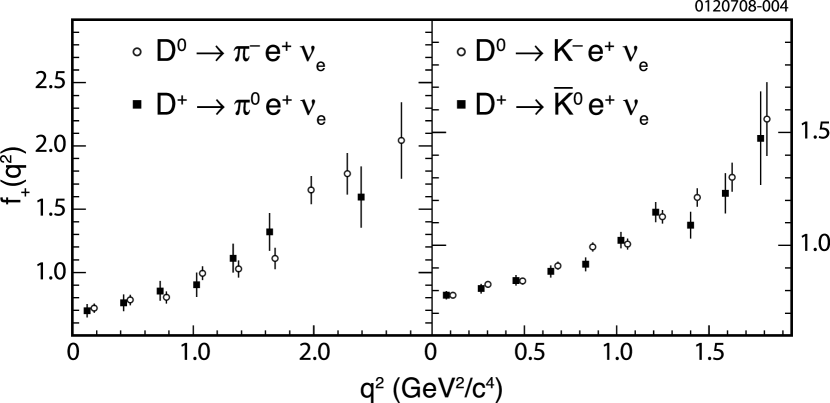
Figure 4: The data displayed as $f_{+}(q^{2})$ for the four semileptonic modes. In each case $f_{+}(q^{2})$ is absolutely normalized. The $D^{+}$ and $D^{0}$ distributions are each offset symmetrically in $q^{2}$ to facilitate display.

VI.2 Fitting the Differential Decay Rate to Determine Form Factors

We use the least squares method to fit the absolutely-normalized efficiency-corrected and background-subtracted $q^{2}$ distributions. A $\chi^{2}$ is constructed from differences between the number of efficiency corrected signal events with a $\bar{D}$ tag in the $i$th $q^{2}$ bin, $N^{i}_{\rm produced}$, and the theoretically predicted number of events in the $i$th $q^{2}$ bin, $N_{\rm predicted}^{i}$, for a given set of form factor parameters, where $N_{\rm predicted}^{i}$ is obtained using

$$N_{\rm predicted}^{i} =\hskip 142.26378pt$$

$$N_{\rm tag}\tau_{D} \displaystyle\int_{q^{2}_{\rm min}(i)}^{q^{2}_{\rm max}(i)}\frac{G^{2}_{F}|V_{cq}|^{2}p^{3}_{K,\pi}}{24\pi^{3}}|f_{+}(q^{2},{\vec{\theta}})|^{2}dq^{2},$$ (33)

and where $\tau_{D}$ is the lifetime of the relevant $D$ meson, and $\vec{\theta}$ is the vector of form factor parameters that govern the decay rate. Taking into account the correlations among the bins and the correlations among the elements of the inverted efficiency matrix errors , the $\chi^{2}$ is given by

$$\chi^{2} = \sum_{ij}([N_{\rm produced}^{i}]-[N_{\rm predicted}^{i}])$$ (34)

$$\qquad A_{ij}^{-1}([N_{\rm produced}^{j}]-[N_{\rm predicted}^{j}]),$$

where $A_{ij}$ is

$$A_{ij}=\sum_{k}\epsilon^{-1}_{ik}\epsilon^{-1}_{jk}\sigma_{N_{\rm tag,SL}^{k}}^{2}.$$ (35)

Systematic uncertainties and correlations among them are not included in the fit. Instead a systematic uncertainty from each source is estimated separately. The fitting procedure has been tested using ensembles of fits to 100 mock data samples that each correspond to the same integrated luminosity as the data, for a wide range of values of the form factor parameters. It has been established that the statistical uncertainties from this fitting procedure are consistent with the smallest statistical uncertainties expected from a fit, estimated using the Cramer - Rao inequality eadie , and that the fit is consistent with being unbiased.

Fits to the data are made for two parameters related to the shape and the normalization of the $f_{+}(q^{2})$ form factors for the series parametrization, the simple pole, the modified pole model, and the ISGW2 model. For the series parametrization we also present results of fits for three parameters, where the third parameter is a second shape parameter. As an example, Fig. 5 shows simultaneous fits to modes related by isospin symmetry. Before presenting numerical results of the form factor measurements, we describe a study of systematic uncertainties in the next section.

Figure 5: Simultaneous three parameter fits to the background-subtracted, efficiency-corrected and absolutely-normalized data derived decay rates for modes related by isospin $D^{0}\to\pi^{-}e^{+}\nu_{e};D^{+}\to\pi^{0}e^{+}\nu_{e}$, and $D^{0}\to K^{-}e^{+}\nu_{e};D^{+}\to\bar{K}^{0}e^{+}\nu_{e}$. The $D^{+}\to\pi^{0}e^{+}\nu_{e}$ distribution is scaled by a factor two to account for isospin. The series parametrization with a quadratic term is used for these fits. The fit result is the line.

VI.3 Study of Systematic Uncertainties for ${d\Gamma}/{dq^{2}}$ and Form Factor Measurements

VI.3.1 Systematic Uncertainties for ${d\Gamma}/{dq^{2}}$ in $q^{2}$ bins

Each source contributing systematic uncertainty to the absolute branching fractions also contributes systematic uncertainty to measurements of the partial rate ${d\Gamma}/{dq^{2}}$ in $q^{2}$ bins. Procedures identical to those used in the absolute branching fraction measurements are employed to estimate systematic uncertainties for ${d\Gamma}/{dq^{2}}$. In addition, there is a systematic uncertainty associated with imperfect knowledge of $D^{0}$ and $D^{+}$ meson lifetimes. Table 14 reports total systematic uncertainties, and the separated correlated and uncorrelated components, for ${d\Gamma}/{dq^{2}}$ in $q^{2}$ bins for the four semileptonic modes.

Table 14: Correlated, uncorrelated and total systematic uncertainties in ${d\Gamma}/{dq^{2}}$ for each $q^{2}$ bin for the four semileptonic modes. The $q^{2}$ bins are defined in Table 9.

		Uncertainty (%)
Mode	Type		Bin 1	Bin 2	Bin 3	Bin 4	Bin 5	Bin 6	Bin 7	Bin 8	Bin 9	Bin 10
	Correlated		1.5	1.7	1.8	1.9	1.8	1.8	1.8	1.8	2.0
$D^{0}\rightarrow\pi^{-}e^{+}\nu_{e}$	Uncorrelated		0.5	0.4	0.5	0.5	0.6	0.6	0.6	0.8	1.1
	Total		1.6	1.8	1.9	1.9	1.9	1.9	1.9	1.9	2.3
	Correlated		6.8	6.1	5.4	4.8	4.2	3.6	3.1
$D^{+}\rightarrow\pi^{0}e^{+}\nu_{e}$	Uncorrelated		0.7	0.8	0.8	0.9	0.9	1.0	0.9
	Total		6.8	6.1	5.4	4.9	4.3	3.8	3.2
	Correlated		1.4	1.5	1.6	1.6	1.7	1.8	1.8	1.7	1.9	1.5
$D^{0}\rightarrow K^{-}e^{+}\nu_{e}$	Uncorrelated		0.4	0.4	0.4	0.4	0.4	0.4	0.5	0.7	0.9	1.9
	Total		1.5	1.6	1.7	1.7	1.8	1.8	1.9	1.9	2.1	2.4
	Correlated		2.4	2.5	2.5	2.5	2.6	2.6	2.6	2.7	2.6	2.6
$D^{+}\rightarrow\bar{K}^{0}e^{+}\nu_{e}$	Uncorrelated		0.4	0.4	0.5	0.5	0.6	0.6	0.7	0.9	1.2	2.2
	Total		2.4	2.5	2.5	2.6	2.6	2.7	2.7	2.9	2.9	3.4

Systematic uncertainties associated with finding and identifying the hadron (positron) in the final state of a semileptonic decay are measured in bins of hadron (positron) momentum and propagated to the $d\Gamma/dq^{2}$ distributions. In the rest frame of the decaying $D$ meson, $q^{2}$ is determined by the momentum of the final state hadron. Because $\psi(3770)$ decays produce $D$ mesons with a small boost, $q^{2}$ is strongly correlated with the momentum of the final state hadron measured in the laboratory frame. Therefore systematic uncertainties measured in hadron momentum bins, when propagated to $d\Gamma/dq^{2}$, lead to uncertainties that are mostly uncorrelated between $q^{2}$ bins. The correlation between $q^{2}$ and the positron momentum in the laboratory frame is less pronounced due to additional degrees of freedom associated with the undetected neutrino. Systematic uncertainties in positron momentum bins are therefore averaged over a range in $q^{2}$ and their net effect is to produce uncertainties that are nearly constant and fully correlated between $q^{2}$ bins.

To simplify the estimation of the systematic uncertainties, we assume that a given systematic uncertainty is either fully correlated or uncorrelated between $q^{2}$ bins as discussed in the remainder of this section.

Studies of the momentum dependence of the systematic uncertainty associated with track finding efficiencies are performed in three momentum bins covering the entire momentum range accessible in $D$ meson decays at the $\psi(3770)$. Efficiencies for positively and negatively charged pions and kaons are measured separately. We assume that track finding efficiencies for positrons are identical to those for positively charged pions. A systematic uncertainty from track finding efficiencies in a $q^{2}$ bin is calculated by weighting charged hadron (positron) spectra with the efficiency uncertainties measured in the hadron (positron) momentum bins and summing contributions from different momentum bins. Due to the coarse binning used in the tracking studies and because positron and charged hadron track finding uncertainties are combined in each $q^{2}$ bin, systematic uncertainties associated with track finding efficiency are strongly correlated between $q^{2}$ bins. We assume that they are fully correlated.

Systematic uncertainties associated with charged hadron identification in $D^{0}\rightarrow K^{-}e^{+}\nu_{e}$ $(D^{0}\rightarrow\pi^{-}e^{+}\nu_{e})$ are obtained by weighting charged hadron spectra with the statistical uncertainties associated with charged hadron identification measured in 100 (80)  MeV/$c$ – wide momentum bins and summing contributions from different momentum bins in quadrature. Because the hadron momentum is strongly correlated with $q^{2}$, these systematic uncertainties are largely independent for well-separated values of $q^{2}$. We therefore assume that the systematic uncertainties associated with hadron identification are uncorrelated between $q^{2}$ bins.

The systematic uncertainty in the $\pi^{0}$ reconstruction efficiency varies from 1.3% for low $\pi^{0}$ momenta to 6.3% for high $\pi^{0}$ momenta and is found to be fully correlated between $q^{2}$ bins. Systematic uncertainties associated with the $K^{0}_{S}$ reconstruction are found to be independent of the $K^{0}_{S}$ momentum and are fully correlated between $q^{2}$ bins.

Systematic uncertainties due to simulation of ISR and FSR are strongly correlated between $q^{2}$ bins. Systematic uncertainties from FSR are assigned based on differences between the main results and results of fits with efficiency matrices obtained using a subset of signal MC events without FSR. To evaluate systematic uncertainties associated with ISR, we repeated the analysis with two alternative efficiency matrices: one using signal MC events with soft ISR photons ($E_{\gamma}\leq 25$ keV) and the other from the remainder of the signal MC events. Comparing results of fits with these two efficiency matrices, we conclude that systematic uncertainties due to ISR are negligible.

The background is modeled using the generic MC sample. Systematic uncertainties associated with the modeling of background are obtained by varying the composition of the background sample according to uncertainties in the branching fractions of processes producing background, and by the statistical uncertainties in the normalization for each background component. In addition, in cases where a background component arises from misidentified hadrons or leptons, background normalizations are varied according to the uncertainty in the relative misidentification rates between the data and MC simulation.

Systematic uncertainties from imperfect knowledge of the $D^{0}$ (0.4%) and $D^{+}$ (0.7%) meson lifetimes, the number of tags (0.4%), and unused tracks (0.3%) are fully correlated between $q^{2}$ bins. Systematic uncertainties due to the limited size of the MC samples used to measure the efficiency matrices are statistical in origin and are therefore uncorrelated between $q^{2}$ bins.

Three systematic uncertainties for each $q^{2}$ bin are presented in Table 14. These are the combined sum in quadrature of all correlated and all uncorrelated contributions, and the total systematic uncertainty. The magnitude of the systematic uncertainty in each $q^{2}$ bin is significantly smaller than the corresponding statistical uncertainty, and the relative size of the uncorrelated systematic uncertainty is small compared to the correlated systematic uncertainty in nearly all bins. (Note, in the last $q^{2}$ bin the uncorrelated systematic uncertainty is dominated by uncertainty due to the limited size of the MC sample, and for $D\rightarrow Ke^{+}\nu_{e}$ it is comparable to the correlated systematic uncertainty.) For comparison to theory and for the form factor measurements presented here we assume that systematic uncertainties are fully correlated between $q^{2}$ bins.

VI.3.2 Systematic Uncertainties for Measurements of $f_{+}(0)$ and Form Factor Shape Parameters

The normalization parameter, $f_{+}(0)|V_{cq}|$, and form factor shape parameters are determined from simultaneous two parameter fits to $d\Gamma/dq^{2}(q^{2})$ for each isospin conjugate semileptonic mode. In each case the correlation coefficient between the form factor shape parameter and the normalization parameter is found to be small.

Systematic uncertainties associated with the absolute form factor normalization, $f_{+}(0)$, for each semileptonic mode, are one half the systematic uncertainties in the branching fraction measurements presented in Sec. V.2 combined in quadrature with the small uncertainties associated with the knowledge of $D^{0}$ (0.4%) and $D^{+}$ (0.7%) PDG2004 lifetimes and the CKM matrix elements $|V_{cs}|$ (0.1%) and $|V_{cd}|$ (1.3%) obtained from the unitarity constraints of the CKM matrix.

Systematic uncertainties for form factor shape parameters are obtained from one parameter fits with absolute normalizations fixed. In the rest of this section, we describe sources of systematic uncertainty for form factor shape parameters and how they are estimated.

A systematic uncertainty associated with the fit procedure is assigned by examining the pull distributions resulting from fits to ensembles of mock data samples. The studies determine that the fit has good fidelity, and place an upper limit on the existence of bias at 15% of the statistical uncertainty in the measurement on data, which we take as a systematic uncertainty associated with the fit method (Table 15).

As discussed in the previous section, most sources of systematic uncertainty are $q^{2}$ independent and, consequently, do not contribute a systematic uncertainty in the form factor shape parameter measurement. Accordingly, to assign systematic uncertainties for tracking efficiency, $K_{S}^{0}$ and $\pi^{0}$ finding, and hadron and electron identification, a correlation with particle momentum consistent with our knowledge of each systematic effect is introduced. This is achieved by constructing a model according to which each systematic uncertainty varies linearly as a function of the particle momentum. The slope for each systematic uncertainty is determined by the precision with which each systematic effect is known. We fit the data using efficiency matrices modified according to this model. We also construct a set of mock data samples for each source using the model and fit them to obtain systematic uncertainties for the form factor shape parameters. We find that systematic uncertainties measured by these two methods are consistent.

Systematic uncertainties associated with the simulation of FSR and from background estimation are obtained as described in the previous section. The total systematic uncertainty, given in Table 15, ranges from 19% to 53% of the statistical uncertainty. The ratio of the systematic to statistical uncertainties for shape parameters are found to be consistent for all parametrizations.

Table 15: Systematic uncertainties for form factor shape parameters in units of the statistical uncertainty of the measurement with data. The modes are labeled by their final state hadrons.

		Systematic uncertainty ($\sigma_{stat}$)
Sources		$K^{-}$	$K_{S}^{0}$	$\pi^{-}$	$\pi^{0}$
Track finding		$0.03$	$0.00$	$0.02$	$0.00$
$K_{S}^{0}$ finding		$0.00$	$0.20$	$0.00$	$0.00$
$\pi^{0}$ finding		$0.00$	$0.00$	$0.00$	$0.38$
Hadron ID		$0.11$	$0.00$	$0.05$	$0.00$
Electron ID		$0.02$	$0.01$	$0.01$	$0.01$
FSR		$0.20$	$0.16$	$0.07$	$0.04$
Background		$0.05$	$0.07$	$0.06$	$0.34$
MC size		$0.10$	$0.10$	$0.05$	$0.05$
Fitter		$0.15$	$0.15$	$0.15$	$0.15$
Total		$0.30$	$0.32$	$0.19$	$0.53$

VI.4 Form Factor Measurement Results

The fit described in Sec. VI.2 is applied to the decay rates in Table 12 for each semileptonic mode and to pairs of modes related by isospin. Five fits are carried out per mode. In each case the normalization parameter $f_{+}(0)|V_{cq}|$ and one or more form factor shape parameters are determined. Specifically the shape parameters are $M_{\rm pole}$ (simple pole model), $\alpha$ (modified pole model), and $r$ (ISGW2). For the series parametrization we map the data to the variable $z$. The quantity $P(z)\phi(z)f_{+}(z)$ is, by convention, constrained to unity at $z=z_{\rm max}$, which corresponds to $q^{2}=0$. We fit to the distribution $d\Gamma/dq^{2}=(G_{F}^{2}/24\pi^{3})p^{3}_{K,\pi}|V_{cq}|^{2}a_{0}^{2}F_{+}^{2}(z)$, where: $F_{+}(z)=[P(z)\phi(z)]^{-1}\times(1+r_{1}z+r_{2}z^{2})$ with $r_{1}=a_{1}/a_{0}$, $r_{2}=a_{2}/a_{0}$, and $f_{+}(q^{2})=a_{0}F_{+}(z)$.

The fit returns the normalization parameter $f_{+}(0)|V_{cq}|$ and either $r_{1}$ or $r_{1}$ and $r_{2}$. We test the sensitivity of the data to the number of parameters and the convergence of the series. For the series parametrization the slope at the intercept, $1+1/\beta-\delta$, is also reported. Results of fits to each parametrization are given in Table 16 and Table 17.

Comparisons of four of the five fits to the data for each of the four modes are shown in Fig. 6 (ISGW2 is excluded). To facilitate a comparison, in Fig. 7 we normalize each fit to the result of the three parameter series fit. It can be seen that each of these parametrizations provides an adequate, and almost identical, description of the data when the shape parameter is allowed to be free. To illustrate the difference between the linear and quadratic $z$-expansion fits, Fig. 8 shows $P(z)\phi(z)f_{+}(z)/P(z(q^{2}=0))\phi(z(q^{2}=0))$ for both as a function of $z$.

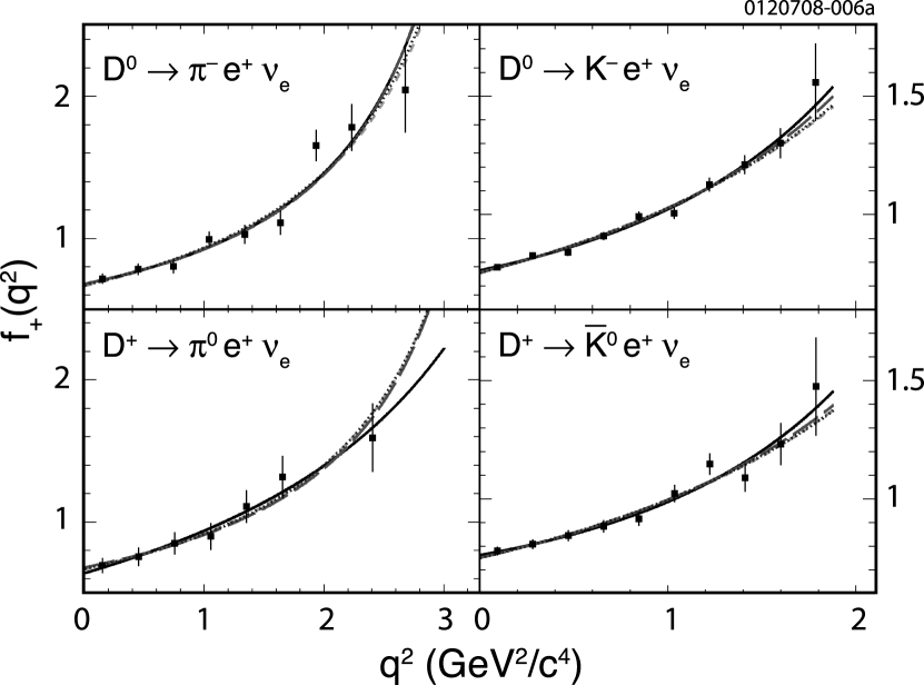
Figure 6: Projections of fits onto $f_{+}(q^{2})$ for each semileptonic mode. In each case $f_{+}(q^{2})$ is absolutely normalized. The data are shown as points with error bars. The lines are fits to the simple pole model (long dash), the modified pole model (short dash), the series parametrization with two free parameters (dot), and the series parametrization with three free parameters (solid).

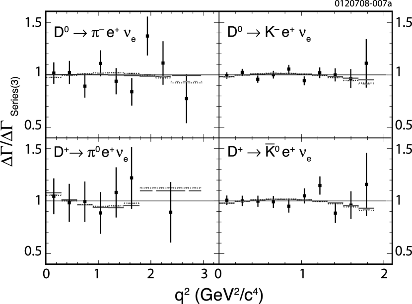
Figure 7: Form factor fit comparison for each semileptonic mode. All data (squares) and fits (histograms) are normalized to the relevant three parameter fit result (Series (3) solid line at unity). The simple pole, modified pole, and two parameter series fit (Series (2)) are represented by long dash, short dash, and dotted histograms, respectively.

An independent assessment of the quality of the fits to the data is obtained from the ability of the fit to describe distributions in the data in two variables that are not used to constrain the fit. The first variable is the angle between the $W^{+}$ in the $D$ meson frame and the positron in the $W^{+}$ frame, $\theta_{We}$. The second variable is the laboratory momentum of the positron, $|\vec{p}_{e}|$. Figure 9 shows distributions for $\cos{\theta_{We}}$ and $|\vec{p}_{e}|$ in data and the projections of the fit, where the background contributions are shown as hatched histograms. The fits describe the distributions in these two variables well.

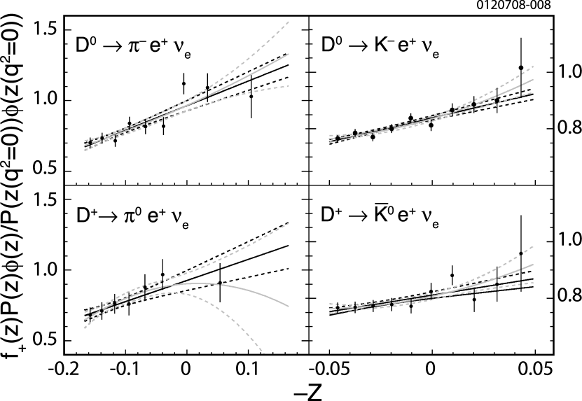
Figure 8: Series parametrization form factor fit comparison to the data for two and three expansion parameters for each semileptonic mode. Series(2) (black line) with $\pm 1\sigma$ uncertainty (black dashed lines). Series (3) (gray line) with $\pm 1\sigma$ uncertainty (gray dashed lines).

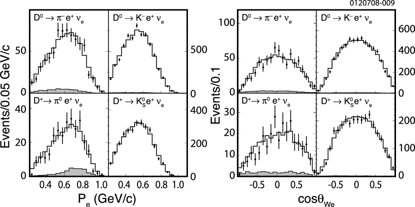
Figure 9: Distributions of positron momenta (left) and $\cos{\theta_{We}}$ (right) in data (points with error bars) and the projection of the fit (solid line) for each semileptonic mode. The background contributions are the hatched histograms.

Table 16: Summary of results of form factor fits to the data: the normalization parameters $f^{K}_{+}(0)|V_{cs}|$ or $f^{\pi}_{+}(0)|V_{cd}|$, shape parameters ($M_{\rm pole}$, $\alpha$, $r$, and $r_{1}$), and the correlation coefficient $\rho$ between the normalization and shape parameters for each fit. The last column gives the $\chi^{2}$ per degree of freedom for each fit.

Simple pole	$f_{+}(0)|V_{cq}|$	$M_{\rm pole}$	$\rho$	$\chi^{2}$ per d.o.f.
$D^{0}\rightarrow\pi^{-}e^{+}\nu_{e}$	0.152(4)(1)	1.94(4)(1)	0.68	1.26
$D^{+}\rightarrow\pi^{0}e^{+}\nu_{e}$	0.153(7)(5)	1.99(10)(5)	0.68	0.37
$D^{0}\rightarrow K^{-}e^{+}\nu_{e}$	0.736(7)(6)	1.95(4)(1)	0.78	0.81
$D^{+}\rightarrow\bar{K}^{0}e^{+}\nu_{e}$	0.733(11)(9)	2.02(6)(2)	0.78	0.80
$D\rightarrow\pi e^{+}\nu_{e}$	0.152(4)(1)	1.95(4)(2)	0.68	0.82
$D\rightarrow Ke^{+}\nu_{e}$	0.735(7)(5)	1.97(3)(1)	0.78	1.00
Mod.pole	$f_{+}(0)|V_{cq}|$	$\alpha$	$\rho$	$\chi^{2}$ per d.o.f.
$D^{0}\rightarrow\pi^{-}e^{+}\nu_{e}$	0.150(6)(1)	0.18(12)(4)	-0.83	1.26
$D^{+}\rightarrow\pi^{0}e^{+}\nu_{e}$	0.151(9)(4)	0.09(22)(12)	-0.80	0.35
$D^{0}\rightarrow K^{-}e^{+}\nu_{e}$	0.733(8)(6)	0.25(6)(2)	-0.83	0.94
$D^{+}\rightarrow\bar{K}^{0}e^{+}\nu_{e}$	0.732(12)(9)	0.12(10)(4)	-0.82	0.83
$D\rightarrow\pi e^{+}\nu_{e}$	0.150(5)(2)	0.16(10)(5)	-0.81	0.78
$D\rightarrow Ke^{+}\nu_{e}$	0.733(7)(6)	0.21(5)(2)	-0.83	1.01
ISGW2	$f_{+}(0)|V_{cq}|$	$r(ISGW2)$	$\rho$	$\chi^{2}$ per d.o.f.
$D^{0}\rightarrow\pi^{-}e^{+}\nu_{e}$	0.147(5)(1)	1.98(12)(2)	-0.80	1.37
$D^{+}\rightarrow\pi^{0}e^{+}\nu_{e}$	0.149(8)(4)	1.85(22)(12)	-0.77	0.26
$D^{0}\rightarrow K^{-}e^{+}\nu_{e}$	0.730(8)(6)	1.56(4)(1)	-0.81	1.07
$D^{+}\rightarrow\bar{K}^{0}e^{+}\nu_{e}$	0.723(12)(9)	1.48(7)(2)	-0.81	0.91
$D\rightarrow\pi e^{+}\nu_{e}$	0.147(4)(2)	1.95(10)(5)	-0.80	0.80
$D\rightarrow Ke^{+}\nu_{e}$	0.730(7)(6)	1.53(4)(2)	-0.81	1.09
Series (2 param.)	$f_{+}(0)|V_{cq}|$	$r_{1}$	$1+1/\beta-\delta$	$\rho$	$\chi^{2}$ per d.o.f.
$D^{0}\rightarrow\pi^{-}e^{+}\nu_{e}$	0.150(6)(1)	-1.80(27)(5)	1.00(11)(2)	0.84	1.26
$D^{+}\rightarrow\pi^{0}e^{+}\nu_{e}$	0.151(9)(4)	-1.57(49)(26)	0.92(17)(9)	0.81	0.36
$D^{0}\rightarrow K^{-}e^{+}\nu_{e}$	0.734(8)(6)	-1.96(28)(8)	0.89(5)(2)	0.83	0.88
$D^{+}\rightarrow\bar{K}^{0}e^{+}\nu_{e}$	0.733(12)(9)	-1.40(44)(14)	0.79(7)(3)	0.82	0.81
$D\rightarrow\pi e^{+}\nu_{e}$	0.151(5)(2)	-1.75(11)(23)	0.99(9)(4)	0.83	0.78
$D\rightarrow Ke^{+}\nu_{e}$	0.734(7)(6)	-1.78(24)(10)	0.86(4)(2)	0.83	0.98

Table 17: Summary of the results of form factor fits for the series parametrization with three parameters to the data: the normalization parameters $f^{K}_{+}(0)|V_{cs}|$ or $f^{\pi}_{+}(0)|V_{cd}|$, the shape parameters $r_{1}$, and $r_{2}$, and correlation coefficients $\rho_{ij}$ between the parameters determined by the fit. The last column gives the $\chi^{2}$ per degree of freedom for each fit.

Decay	$f_{+}(0)|V_{cq}|$	$r_{1}$	$r_{2}$	$1+1/\beta-\delta$	$\rho_{01}$	$\rho_{02}$	$\rho_{12}$	$\chi^{2}$ per d.o.f.
$D^{0}\rightarrow\pi^{-}e^{+}\nu_{e}$	0.152(8)(1)	-2.0(6)(1)	1.6(4.2)(0.8)	0.91(24)(5)	-0.36	0.67	-0.91	1.45
$D^{+}\rightarrow\pi^{0}e^{+}\nu_{e}$	0.144(12)(4)	-0.3(1.8)(1.0)	-7.9(10.5)(5.6)	1.36(43)(23)	-0.46	0.68	-0.96	0.29
$D^{0}\rightarrow K^{-}e^{+}\nu_{e}$	0.745(12)(6)	-2.4(5)(2)	15.6(12.8)(3.8)	0.70(15)(5)	-0.26	0.71	-0.82	0.79
$D^{+}\rightarrow\bar{K}^{0}e^{+}\nu_{e}$	0.744(17)(9)	-1.9(7)(2)	16.6(19.3)(6.2)	0.61(21)(7)	-0.22	0.71	-0.80	0.82
$D\rightarrow\pi e^{+}\nu_{e}$	0.151(7)(2)	-1.8(6)(3)	0.3(3.9)(1.7)	0.98(23)(10)	-0.38	0.67	-0.92	0.84
$D\rightarrow Ke^{+}\nu_{e}$	0.744(10)(6)	-2.2(4)(2)	16.9(11.4)(4.7)	0.69(12)(5)	-0.25	0.71	0.81	0.93

Using the ISGW2 parametrization we determine the isospin conjugate average values of the meson radius to be

$$r^{K}=1.53(4)(2){\rm~{}GeV}^{-1},$$ (36)

$$r^{\pi}=1.95(10)(5){\rm~{}GeV}^{-1}.$$ (37)

They are the most precise measurements of these quantities to date, and are $18\sigma$ and $5\sigma$ from the ISGW2 expected values $r^{K}=1.12{\rm~{}GeV^{-1}}$ and $r^{\pi}=1.410{\rm~{}GeV^{-1}}$, respectively. We have assigned no uncertainty to the theoretical prediction, and assume here and in what follows, that the experimental uncertainties derived from the fit are Gaussian distributed. A comparison to other recent measurements is given in Table 18. The measurements by BABAR and Belle disagree by $3.8\sigma$. Our measurement of $r^{K}$ is over $4\sigma$ smaller than Belle, and $1.6\sigma$ smaller than BABAR.

Table 18: Compilation of recent measurements of the ISGW2 parameters $r^{K}$ and $r^{\pi}$ in units of GeV^-1.

	$r^{K}$	$r^{\pi}$
Belle BELLE-06	2.47(15)(15)	2.68(45)(40)
BABAR BABAR-06	1.645(36)(44)	–
CLEO-c (tagged)	1.53(4)(2)	1.95(10)(5)

Using the simple pole model, we determine the isospin conjugate average pole masses to be

$$M_{\rm pole}^{K}=1.97(3)(1){\rm~{}GeV}/c^{2},$$ (38)

$$M_{\rm pole}^{\pi}=1.95(4)(2){\rm~{}GeV}/c^{2}.$$ (39)

These values differ by $4.6\sigma$ and $1.3\sigma$ from the well-measured masses: $M_{D_{s}^{*+}}=2112.0\pm 0.6~{}{\rm MeV}/c^{2}$ and $M_{D^{*+}}=2010.0\pm 0.4~{}{\rm MeV}/c^{2}$ PDG2006 , respectively. Comparison to previous measurements are given in Table 19 and Table 20. For $D\rightarrow K\ell^{+}\nu_{\ell}$ all of the more recent measurements are below the mass of the $D_{s}^{*}$ meson. Our measurement of $M_{\rm pole}^{K}$ is in excellent agreement with Ref. Nadia , but is $2.3\sigma$ larger than the BABAR BABAR-06 measurement, and $2.5\sigma$ larger than the Belle BELLE-06 measurement. For $D\rightarrow\pi\ell^{+}\nu_{\ell}$ all measurements are much less precise and are in reasonable agreement, albeit within large uncertainties. All measurements are below the mass of the $D^{*}$ meson.

Table 19: Compilation of measurements of $M_{\rm pole}$ in $D\rightarrow K\ell\nu_{\ell}$. CLEO-c (tagged) is the isospin averaged value; CLEO-c (untagged) is for $D^{0}\rightarrow K^{-}e^{+}\nu_{e}$.

	$M_{\rm pole}^{K}$ ${\rm GeV/c^{2}}$
Mark III MARKIII-91	1.80${}_{-0.20}^{+0.50}$(25)
E691 E691-89	2.10${}_{-0.20}^{+0.40}$(20)
CLEO CLEO-91	2.10${}_{-0.20}^{+0.40}$(25)
CLEOII CLEOII-93	2.00(12)(18)
E687 (Tag) E687-95	1.97${}_{-0.22}^{+0.43}$(7)
E687 (Incl) E687-95	1.87${}_{-0.08}^{+0.11}$(7)
CLEO CLEOIII	1.89(5)${}^{+0.04}_{-0.03}$
FOCUS FOCUS-05	1.93(5)(3)
Belle BELLE-06	1.82(4)(3)
BABAR BABAR-06	1.884(12)(15)
CLEO-c (tagged)	1.97(3)(1)
CLEO-c (untagged) Nadia	1.97(3)(1)

Table 20: Compilation of measurements of $M_{\rm pole}$ in $D\rightarrow\pi\ell\nu_{\ell}$. CLEO-c (tagged) is the isospin average value; CLEO-c (untagged) is for $D^{0}\rightarrow\pi^{-}e^{+}\nu_{e}$.

	$M_{\rm pole}^{\pi}$ ${\rm GeV/c^{2}}$
CLEO (2004) CLEOIII	1.86${}_{-0.06}^{+0.10}$(5)
FOCUS (2004 FOCUS-05 )	1.91${}_{-0.15}^{+0.30}$(7)
Belle (2006) BELLE-06	1.97(8)(4)
CLEO-c (tagged)	1.95(4)(2)
CLEO-c (untagged) Nadia	1.87(3)(1)

Using the modified pole model, we determine the isospin conjugate average shape parameters to be

$$\alpha^{K}=0.21(5)(2),$$ (40)

$$\alpha^{\pi}=0.16(10)(5).$$ (41)

The values of $\alpha^{K}$ and $\alpha^{\pi}$ are $27\sigma$ and $11\sigma$, respectively, from the values of $\sim 1.75$ and $1.34$ required by the BK parametrization. A comparison to previous measurements is given in Table 21. For $Ke^{+}\nu_{e}$ there is excellent agreement between this result and CLEO-c (untagged) Nadia , good agreement with previous measurements by CLEO III CLEOIII , and FOCUS FOCUS-05 , and QCD sum rules QCD-sum-rules-1 , but our result is lower than BABAR BABAR-06 by $2.6\sigma$, lower than Belle BELLE-06 by $2.7\sigma$ and lower than the LQCD fit unquenched_LQCD by $4.2\sigma$. The significance of the discrepancy between our result and the LQCD fit cannot be quantified rigorously, as the covariance matrix for the LQCD form factor is lost during the chiral extrapolation unquenched_LQCD . For $\pi e^{+}\nu_{e}$ there is reasonable agreement with CLEO-c (untagged) Nadia and other previous measurements, albeit within large uncertainties. Our measurement of $\alpha^{\pi}$ is $2.4\sigma$ smaller than the LQCD fit.

Table 21: Compilation of measurements and theoretical predictions for $\alpha^{K}$ and $\alpha^{\pi}$. CLEO-c (tagged) are the isospin average values; CLEO-c (untagged) is for $D^{0}\rightarrow K^{-}e^{+}\nu_{e}$ and $D^{0}\rightarrow\pi^{-}e^{+}\nu_{e}$ respectively.

	$\alpha^{K}$	$\alpha^{\pi}$
FOCUS FOCUS-05	0.28(8)(7)	–
CLEO III CLEOIII	0.36(10)(5)	0.37(25)(15)
Belle BELLE-06	0.52(8)(6)	0.10(21)(10)
BABAR BABAR-06	0.377(23)(29)	–
LQCD unquenched_LQCD	0.50(4)	0.44(4)
LCSR QCD-sum-rules-1	$0.07^{+0.15}_{-0.07}$	$0.01^{+0.11}_{-0.07}$
CQM CQM-alpha	0.24	0.30
CLEO-c (tagged)	0.21(5)(2)	0.16(10)(5)
CLEO-c (untagged) Nadia	0.21(5)(3)	0.37(8)(3)

Fits to the data using the first two terms of the $z$ expansion are reported in Table 16. Fits using the first three terms are given in Table 17 and shown in Fig. 8. The expansion parameters are not predicted. The central value of the ratio of expansion parameters $r_{2}$ is an order of magnitude larger than $r_{1}$, however the statistical uncertainty is of similar magnitude to the central value, and therefore no statement can be made about the convergence of the expansion. Moreover, the data lack the precision, even in the copious $D\rightarrow Ke^{+}\nu_{e}$ mode, to determine $r_{2}$. For this reason there is no appreciable difference between the probability of the $\chi^{2}$ between the two parameter series expansion and three parameter series expansion fits for any mode. The compatibility of the data with linear dependence is consistent with the modified pole ansatz for $f_{+}(q^{2})$. Recently BABAR BABAR-06 using a data sample of 75,000 $D^{0}\to K^{-}e^{+}\nu_{e}$ events, found $r_{1}=-2.5(2)(2)$ and $r_{2}=0.6(6)(5)$, and that the differential rate is well-described by the $z$ expansion with only a linear term. The results reported here for $r_{1}$ and $r_{2}$ are in excellent agreement with CLEO-c (untagged) Nadia and agree with BABAR BABAR-06 to better than $2\sigma$ with the precise level depending on the correlation coefficient for the BABAR $r_{1}$ and $r_{2}$ parameters.

The quadratic series expansion fit returns isospin conjugate average values for $1+1/\beta-\delta$ of 0.69(12)(5) and 0.98(23)(10) for $D\rightarrow Ke^{+}\nu_{e}$ and $D\rightarrow\pi e^{+}\nu_{e}$, respectively. These values are $10\sigma$ and $4\sigma$ from the value of $\sim 2$ required by the BK parametrization, and are consistent with the results in Nadia given in Table 22.

Table 22: Compilation of measurements of $1+1/\beta-\delta$ from CLEO-c tagged and untagged Nadia .

	$1+1/\beta-\delta$
	Tagged	Untagged Nadia
$D^{0}\rightarrow\pi^{-}e^{+}\nu_{e}$	0.91(24)(5)	1.30(37)(12)
$D^{+}\rightarrow\pi^{0}e^{+}\nu_{e}$	1.36(43)(23)	1.58(60)(13)
$D^{0}\rightarrow K^{-}e^{+}\nu_{e}$	0.70(15)(6)	0.62(13)(4)
$D^{+}\rightarrow\bar{K}^{0}e^{+}\nu_{e}$	0.61(21)(7)	0.51(20)(4)
$D\rightarrow\pi e^{+}\nu_{e}$	0.98(23)(10)	–
$D\rightarrow Ke^{+}\nu_{e}$	0.69(12)(5)	–

When the shape parameters are not fixed the $q^{2}$ parametrizations of the simple pole model, the modified pole model, the ISGW2 model, and the series expansion with two and three parameters are functionally almost identical over the $q^{2}$ range accessible in $D$ meson semileptonic decay. For this reason each parametrization is able to describe the data with a comparable $\chi^{2}$ probability.

Measurements of $f_{+}(0)|V_{cq}|$ are given in Table 16 for the ISGW2, simple pole, modified pole, and two parameter series parametrization, and in Table 17 for the three parameter series parametrization. As each parametrization is able to describe the data, measurements of $f_{+}(0)|V_{cq}|$ are very similar among parametrizations. For $D\rightarrow Ke^{+}\nu_{e}$ the values of $f^{K}_{+}(0)|V_{cs}|$ span about one half of a statistical sigma between the pole model, modified pole model, and series expansion (linear). However, the fit to the series expansion including a quadratic term returns a value of $f^{K}_{+}(0)|V_{cs}|$ one statistical sigma larger than for the series expansion using a linear term. The statistical uncertainty is also increased by one third.

For $D\rightarrow\pi e^{+}\nu_{e}$ the values of $f^{\pi}_{+}(0)|V_{cd}|$ span a statistical sigma among the pole model, modified pole model, and the series expansion (linear). The fit to the series expansion including a quadratic term returns a value of $f^{\pi}_{+}(0)|V_{cd}|$ that only differs in the least significant digit from the value obtained for the series expansion using a linear term, but the statistical uncertainty is increased by one third.

Using $|V_{cs}|=0.97334\pm 0.00023$ and $|V_{cd}|=0.2256\pm 0.0010$ obtained using CKM unitarity constraints PDG2008 , we calculate $f_{+}(0)$ for each semileptonic mode separately and also for isospin averages. These are presented in Table 23 and compared to previous measurements in Table 24 note:newVcx . The measurement of $f_{+}^{\pi}(0)$ presented here is the most precise to date.

Table 23: Results for $f_{+}(0)$ obtained from fits to five form factor parametrizations. The first uncertainty is statistical, the second is systematic and the third uncertainty is from the relevant CKM matrix element.

.

Mode	Simple Pole	Mod. Pole	ISGW2	Series (2 param.)	Series (3 param.)
$D^{0}\rightarrow\pi^{-}e^{+}\nu_{e}$	0.676(20)(6)(3)	0.666(25)(6)(3)	0.651(23)(6)(3)	0.667(26)(6)(3)	0.675(34)(6)(3)
$D^{+}\rightarrow\pi^{0}e^{+}\nu_{e}$	0.678(32)(17)(3)	0.670(39)(17)(3)	0.660(35)(17)(3)	0.672(40)(17)(3)	0.640(57)(16)(3)
$D^{0}\rightarrow K^{-}e^{+}\nu_{e}$	0.756(7)(6)(0)	0.753(8)(6)(0)	0.750(8)(6)(0)	0.755(8)(6)(0)	0.765(12)(7)(0)
$D^{+}\rightarrow\bar{K}^{0}e^{+}\nu_{e}$	0.753(11)(9)(0)	0.752(12)(9)(0)	0.748(12)(9)(0)	0.753(13)(9)(0)	0.764(18)(10)(0)
$D\rightarrow\pi e^{+}\nu_{e}$	0.676(17)(7)(3)	0.667(21)(7)(3)	0.653(19)(7)(3)	0.668(21)(7)(3)	0.669(29)(7)(3)
$D\rightarrow Ke^{+}\nu_{e}$	0.756(6)(6)(0)	0.753(7)(6)(0)	0.750(7)(6)(0)	0.754(7)(6)(0)	0.764(10)(6)(0)

Table 24: Compilation of measurements and theoretical predictions for $f_{+}^{K}(0)$ and $f_{+}^{\pi}(0)$. For the experimental measurements the first uncertainty is statistical, and the second is systematic. For this work the third uncertainty is from the relevant CKM matrix element. For BABAR the third uncertainty includes contributions from ${\cal B}(D^{0}\rightarrow K^{-}\pi^{+})$, $\tau_{D^{0}}$ and $|V_{cs}|$.

	$f_{+}^{K}(0)$	$f_{+}^{\pi}(0)$
LQCD1 Abada	0.66(4)(1)	0.57(6)(2)
QCD SR QCD-sum-rules-1	0.60(2)	0.50(1)
LCSR1 QCD-sum-rules-2	0.785(11)	0.65(11)
LCSR2 WWZ	0.67(20)	0.67(19)
ISGW2 ISGW2	1.23	–
LQCD2 unquenched_LQCD	0.73(3)(7)	0.64(3)(6)
Belle BELLE-06	0.695(7)(22)	0.624(20)(30)
BABAR BABAR-06	0.727(7)(5)(7)	–
CLEO-c (tagged)	0.764(10)(6)(0)	0.669(29)(7)(3)
CLEO-c average	0.763(7)(6)(0)	0.629(22)(7)(3)

Table 25: Results for $|V_{cs}|$ and $|V_{cd}|$ obtained from fits to five form-factor parametrizations. The first uncertainty is statistical, the second is systematic and the third is from the $f_{+}(0)$ LQCD prediction.

Decay	Simple Pole	Mod. Pole	ISGW2	Series (2 param.)	Series (3 param.)
$D^{0}\rightarrow\pi^{-}e^{+}\nu_{e}$	0.238(7)(2)(25)	0.235(9)(2)(25)	0.230(8)(2)(24)	0.235(9)(2)(25)	0.238(12)(2)(25)
$D^{+}\rightarrow\pi^{0}e^{+}\nu_{e}$	0.239(11)(6)(25)	0.236(14)(6)(25)	0.233(12)(6)(24)	0.236(14)(6)(25)	0.226(20)(6)(24)
$D^{0}\rightarrow K^{-}e^{+}\nu_{e}$	1.008(10)(9)(105)	1.004(11)(9)(105)	1.000(11)(9)(104)	1.006(11)(8)(105)	1.020(16)(9)(106)
$D^{+}\rightarrow\bar{K}^{0}e^{+}\nu_{e}$	1.004(15)(13)(104)	1.003(17)(13)(104)	0.997(16)(13)(104)	1.004(17)(13)(105)	1.019(24)(13)(106)
$D\rightarrow\pi e^{+}\nu_{e}$	0.238(6)(2)(25)	0.235(7)(3)(24)	0.230(7)(3)(24)	0.234(8)(2)(25)	0.236(10)(2)(25)
$D\rightarrow Ke^{+}\nu_{e}$	1.007(8)(8)(105)	1.004(9)(8)(105)	0.999(9)(8)(104)	1.006(9)(8)(105)	1.019(13)(9)(106)

VII Determination of $|V_{cs}|$ and $|V_{cd}|$

Using recent unquenched LQCD calculations of the form factor normalizations unquenched_LQCD we obtain $|V_{cq}|$ for each of the four semileptonic modes and for the isospin averages. These are presented in Table 25 for both pole models, the ISGW2 model and the series expansion with two and three parameters.

As the data do not support the physical interpretation of the shape parameter in the ISGW2, simple pole, and modified pole parametrizations we choose the value of $|V_{cq}|$ obtained with the series expansion as our main result. Although the $|V_{cq}|$ statistical uncertainty is one third larger when data is fit to the series expansion with three parameters, we choose this rather than the results obtained with the fit to two parameters to facilitate comparison with Nadia .

We find $|V_{cd}|=0.238(12)(2)(25)$ for $D^{0}\rightarrow\pi^{-}e^{+}\nu_{e}$, and $|V_{cd}|=0.226(21)(6)(24)$ for $D^{+}\rightarrow\pi^{0}e^{+}\nu_{e}$. We find $|V_{cs}|=1.020(16)(9)(106)$ for $D^{0}\rightarrow K^{-}e^{+}\nu_{e}$, and $|V_{cs}|=1.019(24)(13)(106)$ for $D^{+}\rightarrow\bar{K}^{0}e^{+}\nu_{e}$. In each case the third uncertainty in the determination of the CKM matrix element is from theory. Averaging the $D^{0}$ and $D^{+}$ results and taking into account correlated and uncorrelated uncertainties we find

$$|V_{cd}|=0.236\pm 0.010\pm 0.002\pm 0.025$$ (42)

and

$$|V_{cs}|=1.019\pm 0.013\pm 0.009\pm 0.106,$$ (43)

where the uncertainties are statistical, systematic and theoretical, respectively. The theoretical uncertainty dominates and is expected to be reduced soon. We compare our measurements to other determinations in Table 26 and Table 27. Our determination of $|V_{cs}|$ is consistent with previous measurements, is in good agreement with Nadia , and is the most precise to date. Our determination of $|V_{cd}|$ is in good agreement with the result derived from neutrino-nucleon scattering, it is consistent with Nadia and is the most precise determination from $D$ meson semileptonic decay to date.

Table 26: Compilation of determinations of $|V_{cs}|$. For the $\Gamma(K\ell\nu_{\ell})$ determination we use PDG2000 PDG2000 , as PDG2004 PDG2004 does not quote a value from this technique and subsequent PDG determinations PDG2006 ; PDG2008 include a result obtained from an earlier CLEO-c measurement, the data sample for which is a subset of the data used in this work.

	$|V_{cs}|$
$\Gamma(K\ell\nu_{\ell})$ PDG2000 PDG2000	$1.04\pm 0.16$
Charm tagged $W$ decay PDG2006	$0.94^{+0.32}_{-0.26}\pm 0.14$
$\Gamma(K\ell\nu_{\ell})$BESII BESIIVcs	$1.00\pm 0.05\pm 0.11$
CLEO-c (tagged)	$1.019\pm 0.013\pm 0.009\pm 0.106$
CLEO-c (untagged)	$1.015\pm 0.010\pm 0.011\pm 0.106$
CLEO-c average	$1.018\pm 0.010\pm 0.008\pm 0.106$

Table 27: Comparison of determinations of $|V_{cd}|$.

	$|V_{cd}|$
$\nu d\rightarrow cd$ PDG2006	$0.22\pm 0.011$
CLEO-c (tagged)	$0.236\pm 0.010\pm 0.002\pm 0.025$
CLEO-c (untagged)	$0.217\pm 0.009\pm 0.004\pm 0.023$
CLEO-c average	$0.222\pm 0.008\pm 0.003\pm 0.023$

We also extract the ratio $|V_{cd}|/|V_{cs}|$ from the ratio of measured form factors. From the simultaneous quadratic $z$ expansion fits to isospin conjugate pairs we obtain:

$$\frac{|V_{cd}|f_{+}^{\pi}(0)}{\rule[-2.84526pt]{-2.84526pt}{12.80373pt}|V_{cs}|f_{+}^{K}(0)}=0.203\pm 0.009\pm 0.003,$$ (44)

where the uncertainties are statistical and systematic, respectively, and correlations have been taken into account. We can compare this result to calculations of $f_{+}^{\pi}(0)/f_{+}^{K}(0)$ to obtain the ratio of CKM elements. A recent light cone sum rules (LCSR) calculation obtains Patricia $f_{+}^{\pi}(0)/f_{+}^{K}(0)=0.84\pm 0.04$, from which we find

$$\frac{|V_{cd}|}{|V_{cs}|}=0.242\pm 0.011\pm 0.004\pm 0.012,$$ (45)

where the third uncertainty is from LCSR. This value is in reasonable agreement with Nadia .

VIII CLEO-c Averages

In this section we compute average values of the measurements of branching fractions, form factors and $|V_{cs}|$ and $|V_{cd}|$, obtained in this work (tagged), with previous untagged CLEO-c measurements of the same quantities Nadia . These average values represent the best determinations of the branching fractions, form factors, and $|V_{cs}|$ and $|V_{cd}|$ with the CLEO-c 281 pb^-1 data set.

The analysis of the data, both in this work and in Ref. Nadia , does not support the physical interpretation of the shape parameter in the ISGW2, simple pole, and modified pole parametrization. Accordingly, both here and in Ref. Nadia , the values of $|V_{cq}|$ obtained with the series expansion with a quadratic term are chosen as the primary results. Therefore, in this section we present averages of $|V_{cq}|$ and the shape parameters only for the series expansion with a quadratic term.

To allow external use of the set of partial branching fractions presented in this paper and in Ref. Nadia , we determine the full statistical and systematic uncertainty correlation matrices and present them in Appendix A. These matrices allow for simultaneous fits of the results in this work and in Ref. Nadia to any form factor parametrization to obtain form factor parameters. They also allow for simultaneous fits with other experimental results.

The two analyses use the same data set. The untagged analysis has a significantly higher efficiency, resulting in signal yields $\sim 2.5$ times greater than the tagged analysis, but also has larger backgrounds. Most of the signal events found by the tagged analysis are also found by the untagged analysis, and so the measurements produced by the two analyses are highly correlated.

To compute averages we use error matrices to take into account the correlations between measurements made by the two techniques. The statistical covariance matrix between the two analyses has a 2 $\times$ 2 block form. The diagonal blocks are obtained from the untagged and tagged analyses, respectively. The off-diagonal blocks arise from correlations between the two analyses. As the covariance matrix is symmetric, only one off-diagonal block needs to be determined.

The off-diagonal blocks are computed using a bootstrap bootstrap MC simulation, where 185 data-sized MC samples are constructed. Each sample is created by randomly selecting events from the generic MC sample. Each event cannot appear more than once in a given sample. Each analysis runs on each bootstrap sample and the statistical correlation between the analyses can be measured and the off-diagonal block of the statistical covariance matrix computed.

A systematic correlation matrix is constructed by taking each systematic uncertainty as either 100% correlated or uncorrelated between the two analyses. The complete four-block combined statistical and systematic correlation matrix is used to obtain the averages. A comparison of correlation matrices calculated by this technique to those determined by each analysis is made and good agreement is found.

Consider first the determination of the average branching fractions. The untagged analysis determines the branching fractions from the sum of the partial branching fractions in each $q^{2}$ bin. To treat each analysis similarly the derived branching fractions are computed for the tagged analysis from the partial branching fractions in each $q^{2}$ bin, using the partial rates in Table 12, corrected for the lifetime factors. The derived branching fractions are reported in Table 28, and are consistent with the branching fractions found in Sec. V.

Table 28: The derived absolute branching fractions (in percent) obtained by summing the partial branching fractions in each $q^{2}$ bin, for CLEO-c tagged, untagged Nadia , and the average absolute branching fraction.

	Tagged	Untagged	Average
$\pi^{-}e^{+}\nu_{e}$	0.308(13)(4)	0.299(11)(8)	0.304(11)(5)
$\pi^{0}e^{+}\nu_{e}$	0.379(27)(23)	0.373(22)(13)	0.378(20)(12)
$K^{-}e^{+}\nu_{e}$	3.60(5)(5)	3.56(3)(9)	3.60(3)(6)
$\bar{K}^{0}e^{+}\nu_{e}$	8.87(17)(21)	8.53(13)(23)	8.69(12)(19)

To extract the statistical correlations between the two analyses, both analyses have run on the bootstrap samples. The analysis procedures in each case are identical to those used with data. For each semileptonic mode, and each bootstrap sample, we obtain the partial branching fractions in each $q^{2}$ bin. We sum individual $q^{2}$ bins to obtain the total branching fractions. These are used to calculate the statistical covariance matrices.

Table 29 gives the complete 8 $\times$ 8 statistical correlation matrix. The tagged internal block is diagonal as the branching fractions are uncorrelated with each other. The untagged internal block is obtained from the untagged analysis, where the correlations between the total branching fractions have been computed from those between the individual $q^{2}$ bins. The off-diagonal elements in the off-diagonal blocks are small, so we set them to zero. In so doing, we neglect the statistical correlation from using common tag yields. Performing the averaging procedure with or without these elements produces a negligible difference in the final results.

Table 29: The complete branching fraction statistical correlation matrix. Untagged $q^{2}$ intervals are in columns and tagged $q^{2}$ intervals are in rows. The modes are labeled by their final state hadrons.

		Untagged				Tagged
		$\pi^{-}$	$K^{-}$	$\pi^{0}$	$\bar{K}^{0}$	$\pi^{-}$	$K^{-}$	$\pi^{0}$	$\bar{K}^{0}$
	$\pi^{-}$	1.00	-0.04	-0.02	-0.01	0.60	0.00	0.00	0.00
Untagged	$K^{-}$		1.00	0.00	-0.02	0.00	0.49	0.00	0.00
	$\pi^{0}$			1.00	-0.02	0.00	0.00	0.36	0.00
	$\bar{K}^{0}$				1.00	0.00	0.00	0.00	0.43
	$\pi^{-}$					1.00	0.00	0.00	0.00
Tagged	$K^{-}$						1.00	0.00	0.00
	$\pi^{0}$							1.00	0.00
	$\bar{K}^{0}$								1.00

To be conservative, all of the systematic uncertainties in the tagged analysis are taken to be fully correlated with the corresponding systematic uncertainties in the untagged analysis. The untagged analysis has additional systematic uncertainties which have no analog in the tagged analysis. Accordingly, these are taken to be uncorrelated between the two analyses. A covariance matrix for each systematic uncertainty is then constructed. A 39% correlation between the numbers of charged $D$ and neutral $D$ pairs in the untagged analysis is also taken into account. The complete branching fraction systematic correlation matrix is given in Table 30.

Table 30: The complete branching fraction systematic correlation matrix. The modes are labeled by their final state hadrons.

		Untagged				Tagged
		$\pi^{-}$	$K^{-}$	$\pi^{0}$	$\bar{K}^{0}$	$\pi^{-}$	$K^{-}$	$\pi^{0}$	$\bar{K}^{0}$
	$\pi^{-}$	1.00	0.85	0.32	0.31	0.48	0.46	0.08	0.23
Untagged	$K^{-}$		1.00	0.39	0.37	0.48	0.49	0.08	0.24
	$\pi^{0}$			1.00	0.62	0.24	0.24	0.23	0.18
	$\bar{K}^{0}$				1.00	0.38	0.38	0.10	0.59
	$\pi^{-}$					1.00	0.98	0.33	0.60
Tagged	$K^{-}$						1.00	0.31	0.61
	$\pi^{0}$							1.00	0.21
	$\bar{K}^{0}$								1.00

We fit the 8 branching fractions with the four-block statistical covariance matrix. The fit returns $\chi^{2}/{\rm d.o.f.}=6.7/4$. We then repeat the fit with the four-block combined statistical and systematic correlation matrix to obtain the central values for the averages and the combined statistical and systematic uncertainty. This fit returns $\chi^{2}/{\rm d.o.f.}=2.1/4$. The quadrature difference between the uncertainties obtained in the two fits is used to compute the systematic uncertainty. The results of the fits are reported in Table 28. The averaged branching fractions are more precise than those measured by either the tagged or untagged analysis.

To determine the form factor parameters we perform a simultaneous fit to the ($N_{1}+N_{2}$) partial branching fractions, where $N_{1}$ and $N_{2}$ are the numbers of $q^{2}$ bins in the untagged and tagged analyses, respectively. To improve precision, we also simultaneously fit pairs of modes related by isospin. The corresponding correlation matrix has dimensions ($N_{1}+N_{2}$) $\times$ ($N_{1}+N_{2})=(56\times 56$) as there are 5 bins for each mode in the untagged analysis and (9+7+10+10) bins in the tagged analysis. We give averaged results for the series expansion.

Table 31: Measurements of $f_{+}(0)|V_{cq}|$, $r_{1}$ and $r_{2}$ in CLEO-c tagged, untagged Nadia and the CLEO-c average.

		Tagged	Untagged	Average
	$f_{+}(0)|V_{cq}|$	0.152(8)(1)	0.140(7)(3)	0.142(6)(2)
$D^{0}\to\pi^{-}e^{+}\nu_{e}$	$r_{1}$	-2.0(6)(1)	-2.1(7)(3)	-2.1(5)(1)
	$r_{2}$	1.6(4.2)(0.8)	-1.2(4.8)(1.7)	-0.6(3.5)(0.9)
	$f_{+}(0)|V_{cq}|$	0.745(12)(6)	0.747(9)(9)	0.745(8)(6)
$D^{0}\to K^{-}e^{+}\nu_{e}$	$r_{1}$	-2.4(5)(2)	-2.4(4)(1)	-2.4(4)(1)
	$r_{2}$	15.6(12.8)(3.8)	21(11)(2)	17.9(10.0)(1.9)
	$f_{+}(0)|V_{cq}|$	0.144(12)(4)	0.138(11)(4)	0.140(9)(2)
$D^{+}\to\pi^{0}e^{+}\nu_{e}$	$r_{1}$	-0.3(1.8)(1.0)	-0.2(1.5)(4)	-0.2(1.3)(0.2)
	$r_{2}$	-7.9(10.5)(5.6)	-9.8(9.1)(2.1)	-9.4(7.5)(1.1)
	$f_{+}(0)|V_{cq}|$	0.744(17)(9)	0.733(14)(11)	0.733(13)(9)
$D^{+}\to\bar{K}^{0}e^{+}\nu_{e}$	$r_{1}$	-1.9(7)(2)	-2.8(6)(2)	-2.5(6)(1)
	$r_{2}$	16.6(19.3)(6.2)	32(18)(4)	26.8(15.4)(2.6)
	$f_{+}(0)|V_{cq}|$	0.151(7)(2)		0.142(5)(2)
$D\to\pi e^{+}\nu_{e}$	$r_{1}$	-1.8(6)(3)		-1.7(5)(2)
	$r_{2}$	0.3(3.9)(1.7)		-1.9(3.2)(1.1)
	$f_{+}(0)|V_{cq}|$	0.744(10)(6)		0.743(7)(6)
$D\to Ke^{+}\nu_{e}$	$r_{1}$	-2.2(4)(2)		-2.4(3)(1)
	$r_{2}$	16.9(11.4)(4.7)		20.8(8.3)(2.0)

For the fits to the $q^{2}$ distributions for each mode the untagged and tagged diagonal blocks are again taken from the analysis-determined correlation coefficients from the data yield fits. The bootstrap method determines the off-diagonal block statistical correlation matrix. As the $q^{2}$ binning differs between the two analyses we take into account both the correlations between $q^{2}$ intervals that overlap in the two analyses and the correlations between non-overlapping tagged$-$untagged bins. The off-diagonal block of the ($56\times 56$) statistical correlation matrix may be found in Tables A.1 and A.2. The diagonal untagged block is given in Nadia . The systematic covariance matrix is constructed from the systematic uncertainties in each analysis. The off-diagonal block may be found in Tables A.3 and A.4, the untagged diagonal block is given in Nadia , and the tagged diagonal block may be found in Tables A.5 and A.6.

We first perform the fit with the statistical covariance matrix only, then repeat it with the combined statistical and systematic covariance matrix. The quadrature difference between the uncertainties obtained in the two fits is used to compute the systematic uncertainty. The central values for the averages are taken from the combined statistical and systematic fit and are given in Table 31, and the parameter correlations from the fit with statistical and systematic uncertainties are given in Table 32. Finally, to improve precision, isospin constraints are imposed and we determine form factor parameters for $D\to Ke^{+}\nu_{e}$ and $D\to\pi e^{+}\nu_{e}$ from simultaneous fits to the respective isospin conjugate modes. Results and parameter correlations are shown in Tables 31 and 33, respectively. Using $|V_{cs}|$ and $|V_{cd}|$ values constrained by CKM unitarity PDG2008 , the $f^{K}_{+}(0)$ and $f^{\pi}_{+}(0)$ averages are calculated and reported in Table  24.

Table 32: The parameter correlation coefficients for $f_{+}(0)|V_{cq}|$, $r_{1}$ and $r_{2}$ between the tagged and untagged Nadia CLEO-c analyses. The modes are labeled by their final state hadrons.

		$\pi^{-}$			$K^{-}$			$\pi^{0}$			$\bar{K}^{0}$
		$f_{+}(0)|V_{cq}|$	$r_{1}$	$r_{2}$	$f_{+}(0)|V_{cq}|$	$r_{1}$	$r_{2}$	$f_{+}(0)|V_{cq}|$	$r_{1}$	$r_{2}$	$f_{+}(0)|V_{cq}|$	$r_{1}$	$r_{2}$
	$f_{+}(0)|V_{cq}|$	1.00	-0.38	0.65	0.11	0.01	0.00	0.02	0.00	0.00	0.07	-0.01	0.01
$\pi^{-}$	$r_{1}$		1.00	-0.93	0.01	0.00	0.00	0.01	-0.03	0.02	0.01	0.00	0.00
	$r_{2}$			1.00	0.00	0.00	0.01	0.00	0.01	-0.01	0.01	-0.01	0.01
	$f_{+}(0)|V_{cq}|$				1.00	-0.23	0.59	0.04	0.00	0.00	0.16	0.01	-0.01
$K^{-}$	$r_{1}$					1.00	-0.83	0.00	-0.01	0.01	0.03	-0.03	0.03
	$r_{2}$						1.00	0.00	-0.01	0.01	-0.01	0.03	-0.01
	$f_{+}(0)|V_{cq}|$							1.00	-0.43	0.65	0.03	0.00	0.00
$\pi^{0}$	$r_{1}$								1.00	-0.96	0.01	-0.02	0.01
	$r_{2}$									1.00	-0.01	0.01	-0.01
	$f_{+}(0)|V_{cq}|$										1.00	-0.24	0.62
$\bar{K}^{0}$	$r_{1}$											1.00	-0.81
	$r_{2}$												1.00

Table 33: The parameter correlation coefficients for $f_{+}(0)|V_{cq}|$, $r_{1}$ and $r_{2}$ between the tagged and untagged Nadia CLEO-c analysis with isospin constraints imposed. The modes are labeled by their final state hadrons.

		$\pi$			$K$
		$f_{+}(0)|V_{cq}|$	$r_{1}$	$r_{2}$	$f_{+}(0)|V_{cq}|$	$r_{1}$	$r_{2}$
	$f_{+}(0)|V_{cq}|$	1.00	-0.42	0.66	0.13	0.00	0.01
$\pi$	$r_{1}$		1.00	-0.94	0.01	0.00	0.00
	$r_{2}$			1.00	0.00	0.00	0.01
	$f_{+}(0)|V_{cq}|$				1.00	-0.21	0.55
$K$	$r_{1}$					1.00	-0.81
	$r_{2}$						1.00

The CLEO-c averages are

$$|V_{cd}|=0.222\pm 0.008\pm 0.003\pm 0.023$$ (46)

and

$$|V_{cs}|=1.018\pm 0.010\pm 0.008\pm 0.106,$$ (47)

where the uncertainties are statistical, systematic, and theoretical, respectively. We compare these averages to the untagged and tagged standalone determinations in Table 26 and Table 27. In each case the average value is more precise than that obtained with either analysis. This is the most precise determination of $|V_{cs}|$ to date, and the most precise determination of $|V_{cd}|$ from $D$ meson semileptonic decay to date.

IX Summary

In this paper we have presented precise measurements of the absolute branching fractions of $D^{0}$ decays to $K^{-}e^{+}\nu_{e}$ and $\pi^{-}e^{+}\nu_{e}$ and $D^{+}$ decays to $\bar{K}^{0}e^{+}\nu_{e}$ and $\pi^{0}e^{+}\nu_{e}$, that agree well with world averages PDG2004 and Ref. Nadia . We have combined these measurements to demonstrate that $D$ meson exclusive semileptonic decays to pseudoscalar final states are consistent with isospin invariance.

From the $q^{2}$ spectrum of all four decay modes studied, we have made the most precise determinations of $r^{\pi}$ and $r^{K}$. Our measurement of $r^{K}$ is over $4\sigma$ smaller than Belle BELLE-06 , and $1.6\sigma$ smaller than BABAR BABAR-06 . Our measurement of $M_{\rm pole}^{K}$ ($\alpha^{K}$) is in excellent agreement with Ref. Nadia , but is $2.3\sigma$ larger ($2.6\sigma$ smaller) than the BABAR BABAR-06 measurement, and $2.5\sigma$ larger ($2.7\sigma$ smaller) than the Belle BELLE-06 measurement. Our determinations of $r^{\pi}$, $M_{\rm pole}^{\pi}$ and $\alpha^{\pi}$ are in reasonable agreement with Ref Nadia and other previous measurements. Our measurement of $\alpha^{K}$ ($\alpha^{\pi}$) is more than $4\sigma$ ($2.4\sigma$) smaller than the LQCD fit. However, the discrepancy with LCQD is difficult to quantify because the covariance matrix for the LQCD form factors is lost during the chiral extrapolation procedure for the published analysis unquenched_LQCD . The results reported here for the series expansion parameters $r_{1}$ and $r_{2}$ are in excellent agreement with Ref. Nadia and agree with BABAR BABAR-06 to better than $2\sigma$ with the precise level depending on the correlation coefficient for the BABAR $r_{1}$ and $r_{2}$ parameters.

Our data, and other recent measurements (e.g., Refs. CLEOIII ; FOCUS-05 ; BELLE-06 ; BABAR-06 ) do not support the physical interpretation of the shape parameter in the ISGW2, simple pole, and modified pole parametrizations. Accordingly, the $f_{+}(0)|V_{cq}|$ values obtained when the data is fit with the quadratic series expansion were selected as our primary normalization results. We combined these values with the unitarity of the CKM matrix to make a precise determination of the form factor absolute magnitude $f_{+}^{K}(0)$ and the most precise determination of $f_{+}^{\pi}(0)$. Using unquenched LQCD predictions for $f_{+}^{K}(0)$ and $f_{+}^{\pi}(0)$ we have made the most precise determination of $|V_{cs}|$, and the most precise determination of $|V_{cd}|$ from $D$ semileptonic decays to date. The results agree well with previous measurements using semileptonic decays including Ref Nadia , and agree well with charm-tagged $W$ decay measurements of $|V_{cs}|$ and neutrino based determinations of $|V_{cd}|$.

To allow external use of the set of partial branching fractions presented in this paper and in Ref. Nadia we determined the full statistical and systematic uncertainty correlation matrices. These matrices allow for simultaneous fits of the results of this work and Ref Nadia to any form factor parametrization to obtain form factor parameters. They also allow for simultaneous fits with other experimental results.

Finally, we averaged values of the measurements obtained in this work with Ref. Nadia . These averages represent the best determinations of the branching fractions, form factors and $|V_{cs}|$ and $|V_{cd}|$ with the CLEO-c 281 pb^-1 data set nompoleave . They are the most precise measurements of the absolute branching fractions of $D^{0}$ decays to $K^{-}e^{+}\nu_{e}$ and $\pi^{-}e^{+}\nu_{e}$ and $D^{+}$ decays to $\bar{K}^{0}e^{+}\nu_{e}$ and $\pi^{0}e^{+}\nu_{e}$, and the most precise direct determination of $|V_{cs}|$ and the most precise determination of $|V_{cd}|$ from $D$ semileptonic decay.

CESR has recently collected a larger $\psi(3770)$ data sample. It is expected that this sample will result in a further improvement in measurements of $D^{0}$ and $D^{+}$ semileptonic branching fractions, measurements of the decay form factors, and the CKM matrix elements $|V_{cs}|$ and $|V_{cd}|$ cleoc .

X Acknowledgments

We gratefully acknowledge the effort of the CESR staff in providing us with excellent luminosity and running conditions. D. Cronin-Hennessy and A. Ryd thank the A.P. Sloan Foundation. This work was supported by the National Science Foundation, the U.S. Department of Energy, and the Natural Sciences and Engineering Research Council of Canada.

Appendix A Correlation Matrices

To allow external use of the set of partial branching fractions presented in this paper and Nadia this Appendix contains the statistical and systematic uncertainty correlation matrices. These matrices allow for simultaneous fits of these results with other experimental results to obtain form factor parameters. Sec. VIII describes the procedures that have been used to obtain these matrices.

Table A.1: The untagged-tagged block of the statistical correlation matrix obtained from the bootstrap procedure . Untagged $q^{2}$ intervals are in columns and tagged $q^{2}$ intervals are in rows. The lines indicate mode boundaries. The modes are labeled by their final state hadrons. Within each submode, the $q^{2}$ intervals are ordered from lowest to highest (part I).

		Tagged
		$\pi^{-}$									$K^{-}$
		0.46	0.20	-0.01	0.00	0.00	0.00	0.00	0.00	0.00	-0.01	-0.02	0.00	0.00	0.00	0.00	0.00	0.00	0.00	0.00
		0.00	0.35	0.30	-0.02	0.00	0.00	0.00	0.00	0.00	0.00	0.00	0.00	0.00	0.00	0.00	0.00	0.00	0.00	0.00
	$\pi^{-}$	0.00	-0.02	0.28	0.53	0.01	-0.01	0.00	0.00	0.00	0.00	0.00	0.00	0.00	0.00	0.00	0.00	0.00	0.00	0.00
		0.00	0.00	-0.01	-0.02	0.43	0.20	0.00	0.00	-0.01	0.00	0.00	0.00	0.00	0.00	0.00	0.00	0.00	0.00	0.00
		0.00	0.00	0.00	0.00	-0.01	0.35	0.26	0.15	0.35	0.00	0.00	0.00	0.00	0.00	0.00	0.00	0.00	0.00	0.00
		-0.03	-0.01	0.00	0.00	0.00	0.00	0.00	0.00	0.00	0.25	0.27	0.04	-0.02	-0.01	0.00	0.00	0.00	0.00	0.00
		0.00	0.00	0.00	0.00	0.00	0.00	0.00	0.00	0.00	0.00	0.00	0.44	0.37	0.08	-0.03	-0.01	0.00	0.00	0.00
	$K^{-}$	0.00	0.00	0.00	0.00	0.00	0.00	0.00	0.00	0.00	0.00	0.00	-0.03	-0.03	0.28	0.48	0.13	-0.03	-0.01	0.00
		0.00	0.00	0.00	0.00	0.00	0.00	0.00	0.00	0.00	0.00	0.00	0.00	0.00	-0.02	-0.03	0.28	0.47	0.17	-0.02
Untagged		0.00	0.00	0.00	0.00	0.00	0.00	0.00	0.00	0.00	0.00	0.00	0.00	0.00	0.00	0.00	-0.03	-0.04	0.25	0.23
		0.00	0.00	0.00	0.00	0.00	0.00	0.00	0.00	0.00	0.00	0.00	0.00	0.00	0.00	0.00	0.00	0.00	0.00	0.00
		0.00	0.00	0.00	0.00	0.00	0.00	0.00	0.00	0.00	0.00	0.00	0.00	0.00	0.00	0.00	0.00	0.00	0.00	0.00
	$\pi^{0}$	0.00	0.00	0.00	0.00	0.00	0.00	0.00	0.00	0.00	0.00	0.00	0.00	0.00	0.00	0.00	0.00	0.00	0.00	0.00
		0.00	0.00	0.00	0.00	0.00	0.00	0.00	0.00	0.00	0.00	0.00	0.00	0.00	0.00	0.00	0.00	0.00	0.00	0.00
		0.00	0.00	0.00	0.00	0.00	-0.04	-0.03	-0.02	-0.04	0.00	0.00	0.00	0.00	0.00	0.00	0.00	0.00	0.00	0.00
		0.00	0.00	0.00	0.00	0.00	0.00	0.00	0.00	0.00	0.00	0.00	0.00	0.00	0.00	0.00	0.00	0.00	0.00	0.00
		0.00	0.00	0.00	0.00	0.00	0.00	0.00	0.00	0.00	0.00	0.00	0.00	0.00	0.00	0.00	0.00	0.00	0.00	0.00
	$\bar{K}^{0}$	0.00	0.00	0.00	0.00	0.00	0.00	0.00	0.00	0.00	0.00	0.00	0.00	0.00	0.00	0.00	0.00	0.00	0.00	0.00
		0.00	0.00	0.00	0.00	0.00	0.00	0.00	0.00	0.00	0.00	0.00	0.00	0.00	0.00	0.00	0.00	0.00	0.00	0.00
		0.00	0.00	0.00	0.00	0.00	-0.02	-0.01	-0.01	-0.02	0.00	0.00	0.00	0.00	0.00	0.00	0.00	0.00	-0.02	-0.01

Table A.2: The untagged-tagged block of the statistical correlation matrix obtained from the bootstrap procedure . Untagged $q^{2}$ intervals are in columns and tagged $q^{2}$ intervals are in rows. The lines indicate mode boundaries. The modes are labeled by their final state hadrons. Within each submode, the $q^{2}$ intervals are ordered from lowest to highest (part II).

		Tagged
		$\pi^{0}$							$\bar{K}^{0}$
		0.00	0.00	0.00	0.00	0.00	0.00	0.00	0.00	0.00	0.00	0.00	0.00	0.00	0.00	0.00	0.00	0.00
		0.00	0.00	0.00	0.00	0.00	0.00	0.00	0.00	0.00	0.00	0.00	0.00	0.00	0.00	0.00	0.00	0.00
	$\pi^{-}$	0.00	0.00	0.00	0.00	0.00	0.00	0.00	0.00	0.00	0.00	0.00	0.00	0.00	0.00	0.00	0.00	0.00
		0.00	0.00	0.00	0.00	0.00	0.00	0.00	0.00	0.00	0.00	0.00	0.00	0.00	0.00	0.00	0.00	0.00
		0.00	0.00	0.00	0.00	0.00	-0.03	-0.04	0.00	0.00	0.00	0.00	0.00	0.00	0.00	0.00	-0.02	-0.01
		0.00	0.00	0.00	0.00	0.00	0.00	0.00	0.00	0.00	0.00	0.00	0.00	0.00	0.00	0.00	0.00	0.00
		0.00	0.00	0.00	0.00	0.00	0.00	0.00	0.00	0.00	0.00	0.00	0.00	0.00	0.00	0.00	0.00	0.00
	$K^{-}$	0.00	0.00	0.00	0.00	0.00	0.00	0.00	0.00	0.00	0.00	0.00	0.00	0.00	0.00	0.00	0.00	0.00
		0.00	0.00	0.00	0.00	0.00	0.00	0.00	0.00	0.00	0.00	0.00	0.00	0.00	0.00	0.00	0.00	0.00
Untagged		0.00	0.00	0.00	0.00	0.00	0.00	0.00	0.00	0.00	0.00	0.00	0.00	0.00	0.00	0.00	-0.02	-0.02
		0.28	0.18	-0.02	0.00	0.00	0.00	0.00	0.00	0.00	0.00	0.00	0.00	0.00	0.00	0.00	0.00	0.00
		0.00	0.31	0.27	-0.03	0.00	0.00	0.00	0.00	0.00	0.00	0.00	0.00	0.00	0.00	0.00	0.00	0.00
	$\pi^{0}$	0.00	-0.03	0.12	0.36	0.00	-0.01	0.00	0.00	0.00	0.00	0.00	0.00	0.00	0.00	0.00	0.00	0.00
		0.00	0.00	-0.01	-0.03	0.41	0.13	-0.02	0.00	0.00	0.00	0.00	0.00	0.00	0.00	0.00	0.00	0.00
		0.00	0.00	0.00	0.00	-0.03	0.22	0.30	0.00	0.00	0.00	0.00	0.00	0.00	0.00	0.00	-0.02	-0.01
		0.00	0.00	0.00	0.00	0.00	0.00	0.00	0.34	0.28	0.04	-0.01	-0.01	0.00	0.00	0.00	0.00	0.00
		0.00	0.00	0.00	0.00	0.00	0.00	0.00	0.00	0.00	0.26	0.21	0.09	-0.02	-0.01	0.00	0.00	0.00
	$\bar{K}^{0}$	0.00	0.00	0.00	0.00	0.00	0.00	0.00	0.00	0.00	-0.02	-0.01	0.22	0.39	0.20	-0.02	-0.01	0.00
		0.00	0.00	0.00	0.00	0.00	0.00	0.00	0.00	0.00	0.00	0.00	-0.02	-0.03	0.23	0.26	0.17	-0.03
		0.00	0.00	0.00	0.00	0.00	-0.01	-0.02	0.00	0.00	0.00	0.00	0.00	0.00	-0.02	-0.03	0.33	0.27

Table A.3: The untagged-tagged block of the systematic correlation matrix. Untagged $q^{2}$ intervals are in columns and tagged $q^{2}$ intervals are in rows. The lines indicate mode boundaries. The modes are labeled by their final state hadrons. Within each submode, the $q^{2}$ intervals are ordered from lowest to highest (part I).

		Tagged
		$\pi^{-}$									$K^{-}$
		0.34	0.34	0.33	0.33	0.33	0.32	0.32	0.31	0.29	0.29	0.32	0.33	0.33	0.33	0.33	0.32	0.31	0.30	0.21
		0.44	0.47	0.47	0.47	0.47	0.47	0.47	0.44	0.44	0.32	0.39	0.42	0.44	0.45	0.45	0.45	0.44	0.44	0.28
	$\pi^{-}$	0.39	0.40	0.39	0.39	0.38	0.38	0.38	0.36	0.35	0.33	0.36	0.37	0.38	0.38	0.38	0.38	0.36	0.36	0.24
		0.31	0.32	0.31	0.31	0.31	0.31	0.31	0.29	0.28	0.25	0.28	0.30	0.31	0.31	0.31	0.31	0.30	0.29	0.20
		0.26	0.26	0.26	0.26	0.25	0.25	0.25	0.24	0.23	0.21	0.24	0.25	0.25	0.25	0.25	0.25	0.24	0.24	0.16
		0.37	0.38	0.37	0.37	0.37	0.36	0.36	0.35	0.33	0.37	0.39	0.39	0.39	0.40	0.39	0.39	0.38	0.37	0.27
		0.33	0.34	0.33	0.33	0.33	0.32	0.32	0.31	0.29	0.33	0.35	0.35	0.35	0.35	0.35	0.34	0.34	0.33	0.24
	$K^{-}$	0.33	0.33	0.33	0.33	0.32	0.32	0.32	0.31	0.29	0.34	0.35	0.35	0.35	0.35	0.35	0.34	0.34	0.32	0.24
		0.27	0.27	0.26	0.26	0.26	0.25	0.25	0.25	0.23	0.28	0.29	0.29	0.29	0.29	0.28	0.28	0.27	0.26	0.20
Untagged		0.26	0.27	0.27	0.27	0.26	0.26	0.26	0.25	0.23	0.26	0.27	0.28	0.28	0.28	0.28	0.27	0.27	0.26	0.19
		0.19	0.18	0.18	0.17	0.17	0.16	0.16	0.16	0.14	0.21	0.21	0.20	0.20	0.19	0.19	0.18	0.17	0.16	0.12
		0.14	0.15	0.16	0.16	0.16	0.15	0.15	0.15	0.14	0.14	0.15	0.16	0.16	0.16	0.16	0.16	0.14	0.14	0.09
	$\pi^{0}$	0.09	0.10	0.10	0.10	0.10	0.10	0.10	0.10	0.09	0.08	0.09	0.10	0.10	0.10	0.10	0.10	0.09	0.09	0.06
		0.23	0.23	0.23	0.23	0.22	0.22	0.22	0.21	0.20	0.19	0.21	0.21	0.21	0.22	0.22	0.21	0.20	0.20	0.14
		0.10	0.11	0.11	0.12	0.11	0.12	0.12	0.11	0.11	0.07	0.09	0.10	0.11	0.11	0.11	0.11	0.11	0.12	0.08
		0.24	0.24	0.23	0.23	0.22	0.21	0.21	0.21	0.19	0.27	0.27	0.26	0.26	0.26	0.25	0.25	0.23	0.22	0.17
		0.29	0.29	0.28	0.28	0.28	0.27	0.27	0.26	0.24	0.29	0.31	0.30	0.30	0.30	0.30	0.29	0.28	0.27	0.20
	$\bar{K}^{0}$	0.30	0.30	0.30	0.30	0.29	0.29	0.29	0.28	0.26	0.29	0.31	0.32	0.32	0.32	0.31	0.31	0.30	0.29	0.21
		0.31	0.31	0.31	0.31	0.30	0.30	0.30	0.29	0.27	0.30	0.32	0.32	0.33	0.33	0.32	0.32	0.31	0.30	0.21
		0.23	0.24	0.23	0.23	0.23	0.22	0.22	0.21	0.20	0.22	0.24	0.24	0.24	0.24	0.24	0.23	0.22	0.22	0.15

Table A.4: The untagged-tagged block of the systematic correlation matrix. Untagged $q^{2}$ intervals are in columns and tagged $q^{2}$ intervals are in rows. The lines indicate mode boundaries. The modes are labeled by their final state hadrons. Within each submode, the $q^{2}$ intervals are ordered from lowest to highest (part II).

		Tagged
		$\pi^{0}$							$\bar{K}^{0}$
		0.05	0.07	0.08	0.10	0.11	0.13	0.16	0.16	0.19	0.20	0.20	0.21	0.21	0.21	0.22	0.20	0.17
		0.05	0.09	0.12	0.14	0.16	0.20	0.25	0.14	0.22	0.24	0.26	0.27	0.28	0.28	0.31	0.28	0.23
	$\pi^{-}$	0.05	0.08	0.10	0.12	0.13	0.16	0.19	0.16	0.21	0.22	0.22	0.23	0.24	0.24	0.25	0.22	0.19
		0.03	0.05	0.07	0.08	0.10	0.12	0.15	0.11	0.15	0.17	0.17	0.18	0.19	0.19	0.20	0.18	0.15
		0.02	0.04	0.05	0.07	0.08	0.10	0.12	0.09	0.12	0.13	0.13	0.14	0.14	0.14	0.15	0.14	0.11
		0.05	0.07	0.09	0.11	0.12	0.15	0.18	0.17	0.21	0.21	0.22	0.23	0.23	0.23	0.23	0.21	0.18
		0.05	0.07	0.08	0.10	0.11	0.13	0.16	0.15	0.18	0.19	0.20	0.20	0.21	0.21	0.21	0.19	0.16
	$K^{-}$	0.05	0.07	0.08	0.09	0.11	0.13	0.16	0.16	0.19	0.20	0.20	0.21	0.21	0.21	0.21	0.19	0.16
		0.04	0.05	0.06	0.07	0.08	0.10	0.12	0.13	0.15	0.16	0.16	0.16	0.17	0.17	0.17	0.15	0.13
Untagged		0.03	0.05	0.06	0.07	0.08	0.10	0.13	0.09	0.12	0.12	0.13	0.13	0.14	0.14	0.14	0.13	0.11
		0.23	0.23	0.24	0.24	0.23	0.22	0.20	0.18	0.18	0.17	0.17	0.17	0.17	0.17	0.16	0.15	0.13
		0.16	0.17	0.18	0.18	0.18	0.18	0.18	0.13	0.15	0.15	0.15	0.15	0.16	0.15	0.15	0.14	0.12
	$\pi^{0}$	0.17	0.18	0.18	0.18	0.18	0.17	0.15	0.07	0.09	0.09	0.09	0.09	0.10	0.09	0.10	0.09	0.08
		0.32	0.33	0.33	0.34	0.33	0.32	0.29	0.13	0.15	0.15	0.16	0.16	0.17	0.17	0.17	0.15	0.13
		0.24	0.25	0.25	0.25	0.24	0.23	0.19	0.04	0.06	0.07	0.08	0.08	0.08	0.08	0.09	0.08	0.07
		0.07	0.08	0.09	0.11	0.12	0.14	0.16	0.52	0.52	0.51	0.51	0.50	0.50	0.49	0.47	0.46	0.39
		0.07	0.09	0.11	0.12	0.14	0.16	0.20	0.51	0.53	0.52	0.52	0.52	0.52	0.51	0.49	0.48	0.40
	$\bar{K}^{0}$	0.07	0.09	0.11	0.13	0.15	0.17	0.20	0.50	0.51	0.51	0.52	0.51	0.51	0.51	0.49	0.47	0.40
		0.08	0.10	0.12	0.13	0.15	0.18	0.21	0.46	0.49	0.49	0.49	0.49	0.49	0.48	0.47	0.45	0.38
		0.06	0.07	0.09	0.10	0.12	0.14	0.17	0.34	0.36	0.36	0.36	0.36	0.36	0.35	0.34	0.33	0.28

Table A.5: The tagged block of the systematic correlation matrix. The lines indicate mode boundaries. The modes are labeled by their final state hadrons. Within each submode, the $q^{2}$ intervals are ordered from lowest to highest (part I).

		Tagged
		$\pi^{-}$									$K^{-}$
		1.00	0.93	0.91	0.90	0.89	0.88	0.88	0.85	0.80	0.85	0.91	0.92	0.92	0.92	0.91	0.90	0.87	0.84	0.60
			1.00	0.94	0.94	0.92	0.92	0.92	0.88	0.84	0.81	0.89	0.92	0.93	0.94	0.93	0.92	0.90	0.87	0.61
				1.00	0.93	0.92	0.91	0.91	0.87	0.83	0.79	0.88	0.91	0.92	0.93	0.93	0.91	0.89	0.87	0.60
					1.00	0.92	0.92	0.92	0.88	0.84	0.77	0.87	0.91	0.92	0.93	0.93	0.91	0.89	0.87	0.60
	$\pi^{-}$					1.00	0.90	0.90	0.86	0.83	0.76	0.85	0.89	0.90	0.91	0.91	0.90	0.88	0.86	0.59
							1.00	0.90	0.86	0.83	0.75	0.84	0.88	0.90	0.91	0.91	0.90	0.88	0.86	0.58
								1.00	0.86	0.83	0.75	0.84	0.89	0.90	0.91	0.91	0.90	0.88	0.86	0.58
									1.00	0.79	0.73	0.82	0.86	0.87	0.88	0.87	0.86	0.84	0.82	0.56
Tagged										1.00	0.66	0.75	0.80	0.81	0.82	0.83	0.82	0.80	0.79	0.53
											1.00	0.94	0.91	0.90	0.88	0.86	0.85	0.82	0.77	0.62
												1.00	0.96	0.95	0.94	0.92	0.91	0.89	0.84	0.64
													1.00	0.97	0.96	0.95	0.94	0.92	0.88	0.65
														1.00	0.97	0.96	0.94	0.92	0.89	0.65
	$K^{-}$														1.00	0.96	0.95	0.93	0.90	0.65
																1.00	0.94	0.92	0.89	0.64
																	1.00	0.91	0.88	0.63
																		1.00	0.87	0.63
																			1.00	0.60
																				1.00

Table A.6: The tagged block of the systematic correlation matrix. The lines indicate mode boundaries. The modes are labeled by their final state hadrons. Within each submode, the $q^{2}$ intervals are ordered from lowest to highest (part II).

		Tagged
		$\pi^{0}$							$\bar{K}^{0}$
		0.19	0.25	0.30	0.34	0.40	0.46	0.56	0.46	0.54	0.55	0.57	0.58	0.59	0.58	0.59	0.55	0.46
		0.18	0.25	0.30	0.35	0.40	0.48	0.58	0.43	0.53	0.55	0.57	0.59	0.60	0.60	0.62	0.57	0.48
		0.18	0.24	0.30	0.34	0.40	0.47	0.58	0.41	0.51	0.54	0.56	0.58	0.60	0.59	0.62	0.56	0.47
		0.17	0.24	0.30	0.34	0.40	0.47	0.58	0.40	0.51	0.54	0.56	0.58	0.60	0.59	0.62	0.56	0.47
	$\pi^{-}$	0.17	0.24	0.29	0.34	0.40	0.47	0.57	0.40	0.50	0.53	0.55	0.57	0.59	0.58	0.61	0.56	0.47
		0.17	0.23	0.29	0.34	0.39	0.47	0.57	0.38	0.49	0.53	0.55	0.56	0.58	0.58	0.61	0.55	0.47
		0.17	0.23	0.29	0.34	0.39	0.47	0.57	0.38	0.49	0.53	0.55	0.56	0.58	0.58	0.61	0.55	0.47
		0.16	0.23	0.28	0.32	0.38	0.45	0.55	0.38	0.48	0.51	0.53	0.54	0.56	0.56	0.58	0.53	0.45
		0.15	0.21	0.26	0.31	0.36	0.43	0.52	0.33	0.44	0.47	0.50	0.51	0.53	0.53	0.56	0.51	0.43
		0.19	0.23	0.27	0.31	0.35	0.40	0.48	0.53	0.56	0.55	0.55	0.55	0.55	0.55	0.52	0.50	0.42
		0.19	0.24	0.29	0.33	0.38	0.44	0.53	0.52	0.57	0.58	0.59	0.59	0.60	0.59	0.58	0.55	0.46
		0.19	0.25	0.30	0.34	0.39	0.46	0.56	0.49	0.56	0.58	0.59	0.60	0.61	0.61	0.61	0.57	0.48
		0.19	0.25	0.30	0.34	0.40	0.46	0.57	0.48	0.56	0.58	0.59	0.60	0.62	0.61	0.62	0.58	0.48
	$K^{-}$	0.18	0.24	0.30	0.34	0.40	0.47	0.57	0.47	0.55	0.58	0.59	0.60	0.62	0.61	0.63	0.58	0.49
		0.18	0.24	0.29	0.34	0.40	0.47	0.57	0.45	0.54	0.57	0.59	0.60	0.61	0.61	0.63	0.58	0.48
		0.18	0.24	0.29	0.34	0.39	0.46	0.56	0.44	0.54	0.56	0.58	0.59	0.61	0.60	0.62	0.57	0.48
		0.17	0.23	0.28	0.33	0.38	0.45	0.55	0.42	0.52	0.54	0.56	0.57	0.59	0.58	0.60	0.55	0.47
		0.16	0.22	0.27	0.32	0.37	0.44	0.54	0.39	0.49	0.52	0.54	0.55	0.57	0.57	0.59	0.54	0.46
Tagged		0.12	0.16	0.19	0.22	0.26	0.30	0.37	0.32	0.37	0.38	0.39	0.39	0.40	0.40	0.40	0.38	0.32
		1.00	0.98	0.97	0.95	0.91	0.84	0.67	0.15	0.15	0.15	0.15	0.15	0.15	0.15	0.14	0.14	0.12
			1.00	0.98	0.96	0.93	0.87	0.72	0.17	0.19	0.19	0.19	0.19	0.19	0.19	0.19	0.18	0.15
				1.00	0.97	0.95	0.90	0.77	0.19	0.22	0.22	0.23	0.23	0.23	0.23	0.23	0.22	0.18
	$\pi^{0}$				1.00	0.95	0.91	0.80	0.22	0.25	0.26	0.26	0.26	0.27	0.27	0.27	0.25	0.21
						1.00	0.93	0.85	0.24	0.28	0.29	0.30	0.30	0.31	0.31	0.31	0.29	0.25
							1.00	0.89	0.28	0.33	0.34	0.35	0.35	0.36	0.36	0.37	0.34	0.29
								1.00	0.33	0.39	0.41	0.42	0.43	0.44	0.44	0.45	0.42	0.35
									1.00	0.96	0.94	0.93	0.91	0.90	0.89	0.84	0.82	0.69
										1.00	0.96	0.96	0.95	0.94	0.93	0.89	0.87	0.73
											1.00	0.96	0.95	0.95	0.94	0.91	0.88	0.74
												1.00	0.95	0.95	0.94	0.92	0.88	0.74
	$\bar{K}^{0}$												1.00	0.95	0.94	0.91	0.88	0.74
														1.00	0.94	0.92	0.88	0.74
															1.00	0.91	0.88	0.74
																1.00	0.86	0.72
																	1.00	0.69
																		1.00

References

- (1) M. Kobayashi and T. Maskawa, Prog. Theor. Phys. 49, 652 (1973).
- (2) M. Artuso and E. Barberio, Phys. Lett. B 592, 786 (2004); M. Battaglia and L. Gibbons, Phys. Lett. B 592, 793 (2004).
- (3) D. Cronin-Hennessey et al., [CLEO Collaboration], Phys. Rev. Lett. 100, 251802 (2008), and S. Dobbs et al., [CLEO Collaboration], Phys. Rev. D 77, 112005 (2008).
- (4) J.D. Richman and P. Burchat, Rev. Mod. Phys. 67, 893 (1995) and references therein.
- (5) C. G. Boyd, B. Grinstein and R. F. Lebed, Nucl. Phys. B 461, 493 (1996).
- (6) C. G. Boyd and M. J. Savage, Phys. Rev. D 56, 303 (1997) and references therein.
- (7) M. C. Arnesen, B. Grinstein, I. Z. Rothstein, and I. Z. Stewart Phys. Rev. Lett. 95, 071802 (2005).
- (8) T. Becher and R.J. Hill, Phys. Lett. B 633, 61 (2006).
- (9) N. Isgur and M. B. Wise, Phys. Lett. B 232, 113 (1989); 237, 527 (1990); E. Eichten and B. Hill, Phys. Lett. B 234, 511 (1990); H. Georgi, Phys. Lett. B 240, 447 (1990).
- (10) B. Aubert et al., [BABAR Collaboration], Phys. Rev. D 76, 052005 (2007).
- (11) See, e.g., S. Descotes-Genon and A. Le Yaouanc, J. Phys. G 35, 115005 (2008) .
- (12) G.S. Huang et al., [CLEO Collaboration], Phys. Rev. Lett. 94, 011802 (2005).
- (13) J.M. Link et al., [FOCUS Collaboration], Phys. Lett. B 607, 233 (2005).
- (14) L. Widhalm et al., [Belle Collaboration], Phys. Rev. Lett. 97, 061804 (2006).
- (15) D. Becirevic and A.B. Kaidelov. Phys. Lett, B 478, 417 (2000).
- (16) R. J. Hill, Phys. Rev. D 73, 014012 (2006).
- (17) R. J. Hill, In the Proceedings of 4th Flavor Physics and CP Violation Conference (FPCP 2006), Vancouver, British Columbia, Canada, 9-12 Apr 2006, pp 027 [arXiv:hep-ph/0606023].
- (18) M. Wirbel, B. Stech and M. Bauer, Z. Phys. C 29, 637 (1985); J. G. Korner and G. A. Schuler, Z. Phys. C 38, 511 (1988), Erratum-ibid, C 41, 690 (1988); M. Bauer and M. Wirbel, Z. Phys. C 42, 671 (1989); J. G. Korner, K. Schilcher, M. Wirbel and Y. L. Wu, Z. Phys. C 48, 663 (1990) ; W. Jaus, Phys. Rev. D 41, 3394 (1990); W. Jaus, Phys. Rev. D 53, 1349 (1996) [Erratum-ibid. D 54, 5904 (1996)] ; R. Aleksan, A. Le Yaouanc, L. Oliver, O. P‘ene, and J.-C. Raynal, Phys. Rev. D 51, 6235 (1995); I. L. Grach, I. M. Narodetskii and S. Simula, Phys. Lett. B 385, 317 (1996); H. M. Choi and C. R. Ji, Phys. Lett. B 460, 461 (1999); D. Melikhov and B. Stech, Phys. Rev. D 62, 014006 (2000); G. Amoros, S. Noguera, and J. Portoles, Eur. Phys. J. C 27, 243 (2003); S. Fajfer and J. Kamenik, Phys. Rev. D 71, 014020 (2005).
- (19) N. Isgur, D. Scora, B. Grinstein, and M. B. Wise, Phys. Rev. D 39, 799 (1989).
- (20) D. Scora and N. Isgur, Phys. Rev. D 52, 2783 (1995).
- (21) T. M. Aliev, V. L. Eletsky, and Y. I. Kogan, Sov. J. Nucl. Phys. 40, 527 (1984); P. Ball, V. M. Braun, and H. G. Dosch, Phys. Rev. D 44, 3567 (1991).
- (22) A. Khodjamirian, R. Ruckl, S. Weinzierl, C. W. Winhart, and O. Yakovlev, Phys. Rev. D 62, 114002 (2000).
- (23) J. M. Flynn and C. T. Sachrajda, Heavy Flavours (2nd ed.), ed. by A. J. Buras and M. Linder (World Scientific, Singapore). Published in Adv. Ser. Direct. High Energy Phys. 15, 402 (1998).
- (24) A. Abada, D. Becirevic, P. Boucaud, J. P. Leroy, V. Lubicz, and F. Mescia, Nucl. Phys. B 619, 565 (2001).
- (25) C.T.H. Davies et al. Phys. Rev. Lett. 92, 022001 (2004); Follana, E. et al. [HPQCD and UKQCD Collaborations] Phys. Rev. Lett. 100, 062002 (2008).
- (26) C. Aubin et al., Phys. Rev. Lett. 94, 011601 (2005).
- (27) Y. Kubota et al., Nucl. Instrum. Meth. Phys. Res., Sect. A 320, 66 (1992); D. Peterson et al., Nucl. Instrum. Meth. Phys. Res., Sect. A 478, 142 (2002); M. Artuso et al., Nucl. Instrum. Meth. Phys. Res., Sect. A 554, 147 (2005).
- (28) R. Brun et al., Geant 3.21, CERN Program Library Long Writeup W5013, unpublished.
- (29) D.J. Lange, Nucl. Instrum. Methods Phys. Res. Sect. A 462, 152 (2001).
- (30) J. Adler et al., [Mark III Collaboration], Phys. Rev. Lett. 62, 1821 (1989).
- (31) G.S. Huang et al., [CLEO Collaboration], Phys. Rev. Lett. 95, 181801 (2005); T.E. Coan et al., [CLEO Collaboration], Phys. Rev. Lett. 95, 181802 (2005).
- (32) S. Eidelman et al., [Particle Data Group], Phys. Lett. B 592, 1 (2004).
- (33) Q. He et al. [CLEO Collaboration], Phys. Rev. Lett. 95, 121801 (2005) [Erratum-ibid. 96, 199903 (2006)].
- (34) H. Albrecht et al., [ARGUS Collaboration], Phys. Lett. B 241, 278 (1990).
- (35) Events with extra tracks are generally in the tails of the U distributions. We choose to veto these events rather than to rely on the MC to model them. The estimation of the systematic uncertainty associated with this veto is described in Sec. V.2.
- (36) We use , where PDG2006 .
- (37) E. Barberio and Z. Was, Comput. Phys. Commun. 79, 291 (1994).
- (38) W. M. Yao et al. [Particle Data Group], J. Phys. G 33, 1 (2006).
- (39) C. Amsler et al., [Particle Data Group], Phys. Lett. B 667, 1 (2008).
- (40) W. Ablikim et al., [BES Collaboration], Phys. Lett. B 597, 39 (2004).
- (41) W. Y. Wang, Y. L. Wu, and M. Zhong, Phys. Rev. D 67 014024 (2003).
- (42) M. Ablikim et al.,[BES Collaboration], Phys. Lett. B 608, 24 (2005).
- (43) J.M. Link et al., [FOCUS Collaboration], Phys. Lett. B 598, 33 (2004).
- (44) J.M. Link et al., [FOCUS Collaboration], Phys. Lett. B 607, 51 (2005).
- (45) M. Lefebvre, R.K. Keeler, R. Sobie, and J. White, Nucl. Instrum. Methods A 451, 520 (2000).
- (46) W.T. Eadie et al., Statistical Methods in Experimental Physics, Elsevier, New York, 1988.
- (47) A. Bai et al., [MARK III Collaboration], Phys. Rev. Lett. 66, 1011 (1991).
- (48) J. C. Anjos et al., [E691 Collaboration], Phys. Rev. Lett. 62, 1587 (1989).
- (49) G. Crawford et al., [CLEO Collaboration], Phys. Rev. D 44, 3394 (1991).
- (50) A. Bean et al., [CLEO Collaboration], Phys. Lett. B 317, 647 (1993).
- (51) P. L. Frabetti et al., [E687 Collaboration], Phys. Lett. B 317, 647 (1995).
- (52) D. Melikhov and B. Stech, Phys. Rev. D 62, 014006 (2000).
- (53) The CLEO-c untagged analysis Nadia does not present results. It uses values of and from an earlier PDG summary PDG2006 to extract the parameters in the series parametrization (see Eq. (6)) for each semileptonic mode separately, but does not provide isospin averages.
- (54) D.E. Groom et al., [Particle Data Group], European Physical Journal C15, 1 (2000).
- (55) To obtain we have used the measured from BESII and from unquenched_LQCD .
- (56) P. Ball, Phys. Lett. B 641, 50 (2006).
- (57) B. Efron, Ann. Stat. 7, 1 (1979).
- (58) As we do not present averages with Ref. Nadia for the simple pole and modified pole parametrizations, the results presented in this work for , , , and , should not be considered to supersede those of Ref Nadia .
- (59) CLEO-c/CESR-c Taskforces and CLEO Collaboration, Cornell LEPP Preprint CLNS 01/1742 (2001).