Solving the Crystallographic Phase Problem using Dynamical Scattering in Electron Diffraction

Abstract

Solving crystal structures from kinematical X-ray or electron diffraction patterns of single crystals requires many more diffracted beams to be recorded than there are atoms in the structure, since the phases of the structure factors can only be retrieved from such data if the atoms can be resolved as sharply peaked objects. Here a method is presented by which the fact that multiple scattering encodes structure factor phases in the diffracted intensities is being used for solving the crystallographic phase problem. The retrieval of both amplitudes and phases of electron structure factors from diffraction patterns recorded with varying angle of incidence will be demonstrated. No assumption about the scattering potential itself is being made. In particular, the resolution in the diffraction data does not need to be sufficient to resolve atoms, making this method potentially interesting for electron crystallography of 2-dimensional protein crystals and other beam-sensitive complex structures.

I Introduction

Electron diffraction becomes the method of choice when trying to determine the atomic structure of small crystalline volumes for mainly 3 reasons: a) electrons can be focused into very small probes matching the size of even the smallest volumes of material, b) their scattering strength is several orders of magnitude greater than that of X-rays, and c) in contrast to real-space based techniques, such as direct imaging or ptychography, the signal-to-noise ratio of the data increases linearly with (as opposed to the square root of) the number of unit cells being illuminated coherently. For structure determination of inorganic materials the strong interaction of electrons with the scattering medium is traditionally being viewed as a nuisance because existing methods for solving the phase problem in X-ray crystallography assume kinematic scattering, making these methods generally not directly applicable to (single orientation) electron diffraction intensities. But even when reducing the discrepancy of electron diffraction data with a kinematic model, e.g. by averaging over many different dynamical diffraction conditions as is done in precession electron diffraction Vincent and Midgley (1994), the shape of the crystal may not always permit the collection of diffraction data at a sufficiently high specimen tilt to ensure the high degree of completeness required by kinematic phasing techniques for resulting in a unique structure.

In contrast to kinematical diffraction intensities, which are absolutely insensitive to the phases of the structure factors, dynamical diffraction intensities, as observed in most electron diffraction patterns, are sensitive to the sums of phases of structure factor triplets and higher order multiplets, i.e. sets of structure factors for which the sum of the corresponding reciprocal lattice vectors vanishes Moodie (1972). While this encoding of structure factor phase information in the diffracted intensities is the basis for the refinement of structure factors, e.g. from CBED patterns Zuo and Spence (1991); Zuo et al. (1999), it has inspired also a number of attempts to solve the ’dynamic inversion problem’, i.e. to retrieve structure factor amplitudes and phases from dynamical diffraction intensities alone and deterministically, i.e. without making use of any (decent) starting guess at all Spence et al. (1990); Spence (1998); Allen et al. (1999); Spence et al. (1999); Allen et al. (1998, 2000); Allen and Oxley (2001); Donatelli and Spence (2020); Spence and Donatelli (2021).

Approaches which use the sensitivity of multiple scattering to structure factor phases have proven useful also in X-ray diffraction Chang (1982); Juretschke (1982); Shen (1998). However, in contrast to Xray diffraction, the comparatively flat Ewald sphere describing the scattering of high energy electrons usually causes more than just 3 reflections to be close to the Bragg condition, especially in complex structures, making these methods generally inapplicable for phase determination from electron diffraction data. Also in the field of low energy (reflection) electron diffraction (LEED) dynamical scattering is being applied for solving the phase problem Saldin et al. (2002).

The most significant contributions on the path to solving the dynamic inversion problem from transmission electron diffraction data have arguably been made by teams around Allen Allen et al. (1999, 1998, 2000); Allen and Oxley (2001) and Spence Spence et al. (1990); Spence (1998); Spence et al. (1999); Donatelli and Spence (2020); Spence and Donatelli (2021), inspiring each other and occasionally joining forces (on dynamic inversion from images rather than diffraction patterns) Allen et al. (2001). Spence wrote of himself in a publication appearing in the last year of being among us, that he has worked on this subject for forty years of his life Spence and Donatelli (2021). In addition to some early work on deriving expressions for gradients of the scattering matrix Spence et al. (1990) he has contributed schemes that would exploit the interference in overlapping discs of CBED patterns Spence (1998), or apply the principle of projection onto convex sets Spence et al. (1999). The last one of these approaches was picked up by him again very recently together with Donatelli, overcoming problems in convergence by exploiting the unitarity of matrix exponentials of hermition matrices Donatelli and Spence (2020); Spence and Donatelli (2021). Under the assumption that both, absorption and the contribution of exciting additional diffracted beams to the diffraction intensities upon sequentially bringing all diffracted beams in a diffraction pattern into exact Bragg condition, can be neglected, they have been able to directly map a special tilt series of diffraction intensities to a unique set of structure factors. Again, inspiration from work by the group around Allen seemed important for this success Brown et al. (2018), who have also shown that absorption can be taken into account when making use of all the symmetries of the structure factor matrix Allen et al. (2000).

The work presented here is based on a joint publication of Spence and myself about a fast converging scattering path expansion of dynamical scattering Koch and Spence (2003); Koch (2002). Two different approaches, one based on directly solving the polynomial system of equations that result from this expansion, and a ’stacked scattering matrix’ scheme based on a purely reciprocal space multislice formulation that can be solved by treating it like an artificial neural network, will be introduced. While the first approach requires the sample to be thin enough for kinematical scattering to still dominate the recorded intensities, the latter one is capable of dealing with much thicker samples. Demonstrations of these approaches will be based on simulated data in order to be able to compare to the ground truth in a more quantitative manner.

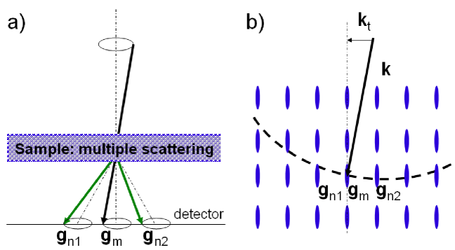
Figure 1: Diagram illustrating the relevant parameters in real (a) and reciprocal space (b). a) In convergent beam electron diffraction (CBED) experiments diffraction patterns for all incident beam directions whose $\vec{k}_{t}$-component lie within a disc are recorded. b) The reciprocal space representation illustrates how changing the incident beam direction causes the Ewald sphere (dashed arch) to intersect the crystal potential reciprocal lattice rods (relrods) with varying excitation errors (deviations from exact Bragg condition along the direction of the surface normal of the sample.

The experimental technique capable of acquiring the type of data that the following two dynamic inversion schemes require as input is large-angle rocking-beam electron diffraction (LARBED) Koch (2011). The advantage of LARBED patterns over conventional convergent-beam electron diffraction (CBED) patterns is that, although the radius of each individual diffraction disc may be several reciprocal lattice vectors (as in large-angle convergent-beam electron diffraction - LACBED), discs produced by the different diffraction spots do not overlap and may therefore be recorded in a single camera exposure. This effect is produced by scanning the angle of incidence on the sample of a nearly parallel beam during the exposure of the recording medium and partially de-scanning it again below the specimen. While the condition of avoiding overlapping discs makes CBED experiments nearly impossible if the unit cell size exceeds 1 nm, being able to control the reciprocal space range covered in LARBED data independent of the unit cell size makes this technique applicable to any material, including beam sensitive materials, since also the size of the illuminating spot may independently be adapted to the grain size of the specimen. A reciprocal-space disc radius larger than half the distance between Bragg spots is also necessary to observe fluctuations in the diffraction intensities across the discs despite the low sample thickness required by the first inversion scheme to keep dynamical diffraction effects at a moderate level. The successful structure factor determination from experimental LARBED data by conjugate-gradient based minimization of the difference squared between the experimental data and a full Bloch wave simulation using 121 measured beams and 456 contributing structure factors has already been demonstrated for the simple centro-symmetric structure of SrTiO₃ and a fitted specimen thickness of 11.3 nm Wang et al. (2016). However, that approach was not yet successful in solving highly complex structures or retrieve structure factors from much thicker samples.

II Expanding the scattering matrix

Without loss of generality it is assumed that the specimen surface normal is parallel to the zone axis as well as the $z$-axis, as illustrated in figure 1. The deviation of the 3-dimensional wave vector of the incident electron beam $\vec{k}=(k_{x},k_{y},k_{z})=(\vec{k}_{t},k_{z})$ from the z-axis is then usually quite small. Based on the Bloch wave solution to the Klein-Gordon equation of high energy scattering of a fast incident beam electron by the crystal potential Fujimoto (1959); Humphreys (1979) the intensity $I_{g_{n}}(\vec{k}_{t})$ of any point in the diffraction pattern defined by the reciprocal lattice vector $\vec{g}_{n}$ of the particular diffraction spot and the tangential component of the incident electron wave vector $\vec{k}_{t}$ is given by the modulus squared of the element of the scattering matrix

$$S(\vec{k}_{t})_{n,m}=[e^{iTA}]_{n,m}$$ (1)

in the $n^{th}$ row and the “central beam” column $m$, i.e. the beam index $m$ for which the reciprocal lattice vector $\vec{g}_{m}=0$. Here $A$ is a square matrix with the potential energy terms $A_{n,m}=U_{\vec{g}_{n}-\vec{g}_{m}}$ as its off-diagonal elements and the (relativistically corrected) terms $\xi_{n}=-(|\vec{g}_{n}|^{2}+2\vec{g}_{n}\cdot\vec{k})/\gamma$ related to the kinetic energy part of the modified Schroedinger equation along its diagonal.

The scalar parameter $T=\pi\gamma\lambda t$ depends on the wavelength $\lambda=(\lambda_{0}^{-2}+U_{0})^{-1/2}\approx\lambda_{0}$ of the incident electron beam corrected by the mean potential $U_{0}$ of the crystal, the specimen thickness $t$, and the relativistic correction factor $\gamma=1+|e|v/m_{0}c^{2}$ (here $m_{0}$ and $e$ are rest mass and charge of the electron and $v$ is the accelerating voltage).

Note that I did not multiply the electron structure factors

$$U_{\vec{g}_{n}-\vec{g}_{m}}=2m_{0}|e|V_{\vec{g}_{n}-\vec{g}_{m}}/h^{2}$$ (2)

in $A$ with the usual relativistic correction factor $\gamma$ but included it in $T$ instead, in order to separate true material constants ($U_{\vec{g}}$) from variable experimental parameters ($\lambda(v),\gamma(v),t,\vec{k}_{t}$). In the above expression

$$V_{\vec{g}}=\Omega^{-1}\int_{cell}V(\vec{r})\exp(2\pi i\vec{g}\cdot\vec{r})d^{3}\vec{r}$$ (3)

are the Fourier coefficients of the crystal potential $V(\vec{r})$, where the integration is over one unit cell, and $\Omega$ is the unit cell volume. The additive constant of $U_{0}$ for every element along the diagonal of $A$ has also been omitted because it only produces a general attenuation of the diffraction pattern due to its imaginary part and a global phase offset due to the real part of $U_{0}$, both unmeasurable in a conventional diffraction experiment.

The crystal potential $V(\vec{r})=V^{r}(\vec{r})+iV^{i}(\vec{r})$ consists of a real part describing the elastic scattering and an imaginary part accounting for inelastic scattering processes which produce a non-isotropic attenuation in the scattered signal, if we collect the zero-loss scattered electrons only, as is routinely done in today’s quantitative (energy filtered) electron diffraction experiments. This means that even for centro-symmetric crystals the $U_{\vec{g}}$ are in general complex, and have a non-zero phase.

It has been shown that the Bloch wave expression (1) can be expanded in a ”scattering path” series Koch and Spence (2003), providing a very general expression which agrees with those derived earlier by analyzing the multiple scattering process directly Cowley and Moodie (1957); Fujiwara (1959); Moodie (1972). Reference Koch and Spence (2003) provides a recursive, but finite explicit expression for the coefficients $C^{q}_{n,l_{1},\ldots l_{q-1},m}(T,\vec{k}_{t})$ in the expansion

$$|S(T,\vec{k}_{t})_{n,m}|^{2}=|e^{T\xi_{n}(\vec{k}_{t})}\delta_{n,m}+\sum_{q=1}^{\infty}\sum_{l_{1}=0}^{N}\sum_{l_{2}=0}^{N}\cdots\sum_{l_{q-1}=0}^{N}$$ (4)

$$\underbrace{U_{\vec{g}_{n}-\vec{g}_{l_{1}}}U_{\vec{g}_{l_{1}}-\vec{g}_{l_{2}}}\cdots U_{\vec{g}_{l_{q-1}}-\vec{g}_{m}}}_{q}C^{q}_{n,l_{1},\ldots l_{q-1},m}(T,\vec{k}_{t})|^{2}$$

for arbitrary scattering path lengths, even in the (degenerate) case of multiple excitation of the same reflection. The interested reader is referred to the original publication Koch and Spence (2003), where the complete expression along with its derivation is provided.

III Inversion by polynomial equation solving

The complex product of any two scattering path coefficients

$$c^{q_{1},q_{2}}_{n,l_{1},\cdots,l_{q_{1}-1},h_{1},\cdots,h_{q_{2}-1}}(T,\vec{k}_{t})=C^{q_{1}}_{n,l_{1},\ldots l_{q_{1}-1},m}(T,\vec{k}_{t})\cdot C^{q_{2}}_{n,h_{1},\ldots h_{q_{2}-1},m}(T,\vec{k}_{t})^{*}$$ (5)

defines the scale and phase factor with which any $q_{1}+q_{2}=q$-monomial of structure factors $U_{\vec{g}_{n}-\vec{g}_{l_{1}}}\cdots U_{\vec{g}_{l_{q_{1}-1}}-\vec{g}_{m}}U^{*}_{\vec{g}_{n}-\vec{g}_{h_{1}}}\cdots U^{*}_{\vec{g}_{h_{q_{2}-1}}-\vec{g}_{m}}$ contributes to the diffraction intensity in the beam $g_{n}$.

The convergence of above scattering path expansion (II) depends on the value of $T=\pi\gamma\lambda t$ and the modulus of the largest structure factor. Increasing the specimen thickness or decreasing the accelerating voltage will therefore increase the largest order of significant monomials in the expansion. We will let $q_{max}$ be the length of the longest scattering path - or, in other words, the largest order of monomial - included in the expansion from here on. The coefficients $c^{q_{1},q_{2}}=c^{q_{1},q_{2}}(T,\vec{k}_{t})$ ($q_{1}+q_{2}\leq q_{max}$, I will omit the functional dependence for increased readability from here on) depend in addition to the specimen thickness and accelerating voltage also on the easily variable experimental parameters $\vec{k}_{t}$. Measuring diffraction intensities for a set of different values of incident electron beam tilt $\vec{k}_{t}$, as in a CBED or LARBED experiment, allows a system of coupled multi-variate polynomial equations of degree $q_{max}$ to be defined whose solution is the set of structure factors which best (in a least squares sense) describe the observed intensities for the set of experimental parameters. The resulting system of equations can be solved by the reformulation-linearization technique Sherali and Tuncbilek (1992) which has been proven to converge to a global optimum.

In order to keep the size of the set of polynomial equations within manageable limits, $T$ should be small enough to let the first term in the expansion, the kinematic scattering intensity at reflection $\vec{g}_{n}$, $n\neq m$,

$$I_{g_{n}}^{(2)}(T,\vec{k}_{t}) = \left|C^{1}_{n,m}(T,\vec{k}_{t})U_{g_{n}}\right|^{2}=\left|\frac{e^{T\xi_{n}}-1}{\xi_{n}}U_{g_{n}}\right|^{2}$$ (6)

$$= c^{1,1}_{n}|U_{g_{n}}|^{2}=\frac{\gamma^{2}\textrm{sin}^{2}(\pi\lambda ts_{g_{n}})}{s_{g_{n}}^{2}}|U_{g_{n}}|^{2}$$

($s_{g_{n}}=\frac{1}{2}\xi_{n}/\gamma$ is also called the excitation error) be the dominant contribution, at least to the strong reflections. Although the kinematic scattering approximation $I_{g_{n}}^{(q_{max}=2)}$ is not sensitive to any structure factor phase invariants, it allows us to define sensible limits on the structure factor amplitude.

It also provides a very simple way of determining the specimen thickness, the only unknown parameter in the $c^{q_{1},q_{2}}$ coefficients (accelerating voltage and incident beam tilt can usually be controlled very precisely). By fitting the (normalized) experimental 2-dimensional rocking curves $I_{g_{n}}(\vec{k}_{t})$ for all reflections with the kinematical one $I_{g_{n}}^{(2)}(T,\vec{k}_{t})$ given by expression (6), both, the specimen thickness as well as a first estimate for the structure factor amplitude can be obtained Koch (2011). The form of expression (6) allows this fit to be implemented very efficiently as a simple one-parameter search in the specimen thickness $t$. The structure factor amplitudes are then determined directly by linear regression for each trial value of $t$. This is, by the way, a much more precise measurement of structure factor amplitudes than using the integrated rocking curve as is done in precession electron diffraction Vincent and Midgley (1994).

Setting $q_{max}=3$ the scattering intensity at reflection $\vec{g}_{n}$ ($n\neq m$) becomes

$$I_{g_{n}}^{(3)}(T,\vec{k}_{t}) = c^{1,1}_{n}|U_{g_{n}}|^{2}+\sum_{l}c^{2,1}_{n,l}U_{\vec{g}_{n}-\vec{g}_{l}}U_{\vec{g}_{l}}U_{\vec{g}_{n}}^{*}+$$

$$\sum_{k}c^{1,2}_{n,h}U_{\vec{g}_{n}}U_{\vec{g}_{n}-\vec{g}_{h}}^{*}U_{\vec{g}_{h}}^{*}$$

$$= I_{g_{n}}^{(2)}(T,\vec{k}_{t})+2\textrm{Re}\left[\sum_{l}c^{2,1}_{n,l}U_{\vec{g}_{n}-\vec{g}_{l}}U_{\vec{g}_{l}}U_{\vec{g}_{n}}^{*}\right]$$

The monomials $U_{\vec{g}_{n}-\vec{g}_{l}}U_{\vec{g}_{l}}U_{\vec{g}_{n}}^{*}$ can be written as the product of the 3 structure factor amplitudes and a phase factor whose argument is the 3-phase invariant $\phi_{\vec{g}_{n}-\vec{g}_{l}}+\phi_{\vec{g}_{l}}-\phi_{\vec{g}_{n}}$, indicating that $I_{g_{n}}^{(3)}(T,\vec{k}_{t})$ must also be sensitive to these phase invariants.

The reformulation-linearization technique developed by Sherali and Tuncbilek Sherali and Tuncbilek (1992) converts the non-linear polynomial equations into linear ones by treating each monomial as an independent variable. By defining additional linear equations that result from obvious relationships between the monomials as well as inequalities produced by upper and lower bounds on the variables, the polynomial set of equations is converted into a set of linear equalities and inequalities for which a solution can be found, if one exists, using standard linear programming algorithms. Once a solution has been found, the limits on the variables may be readjusted (”branch and bound”), resulting in a new linear programming problem and eventually the global solution.

If the initial estimate of the structure factor amplitudes is fairly reliable, the limits within which the correct structure factor amplitude must lie may be defined rather tightly. It is then very likely that the correct solution will be found already in the first linearization step, as has been the case for the test case described below.

In order to verify the performance of the phase retrieval method described above it has been tested using simulated electron diffraction data. Since it has already been shown that Friedel asymmetries in dynamical diffraction patterns of non-centrosymmetric structures can be used to solve the phase problem in the framework of this expansion Koch (2005), I used simulated diffraction patterns of Si in the (110) projection, a simple centro-symmetric structure for demonstration purposes. If absorption is neglected, as has been done for this test case, kinematic and higher order scattering contributions to the diffraction intensities cannot be separated simply on the basis of their symmetry, as it is partly the case for non-centro-symmetric structures Koch (2005), making the reconstruction of centro-symmetric structures even more challenging. In the remainder of this section I demonstrate the direct retrieval of the structure factors of silicon from simulated LARBED data.

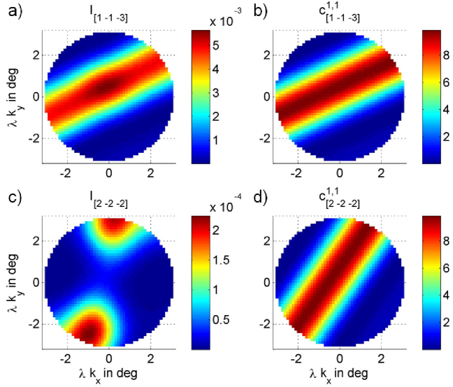
Figure 2: a) Simulated LARBED disc for $\vec{g}=[1\bar{1}\bar{3}]$. b) The coefficient $c^{1,1}_{[1\bar{1}\bar{3}]}(t=3.985\textrm{nm},\vec{k}_{t})$ given by expression 6 (unscaled kinematic rocking curve). The square root of the proportionality constant between the 2 plots shown in a) and b) provides a first estimate of the structure factor amplitude for this reflection. c) Simulated LARBED disc for the kinematically forbidden reflection $[2\bar{2}\bar{2}]$. Comparing the diffraction intensity of a forbidden reflections with the corresponding kinematic rocking curve (d) allows its identification as being forbidden to be automated.

LARBED disc intensities for the following 27 beams have been computed by Bloch wave simulation: $[\bar{2}22]$, $[\bar{2}2\bar{2}]$, $[00\bar{2}]$, $[\bar{3}31]$, $[\bar{3}3\bar{1}]$, $[\bar{2}24]$, $[\bar{2}2\bar{4}]$, $[\bar{1}13]$, $[\bar{1}1\bar{3}]$, $[00\bar{4}]$, $[\bar{2}20]$, $[\bar{1}11]$, $[\bar{1}1\bar{1}]$, $[000]$, $[1\bar{1}1]$, $[1\bar{1}\bar{1}]$, $[2\bar{2}0]$, $[004]$, $[1\bar{1}3]$, $[1\bar{1}\bar{3}]$, $[2\bar{2}4]$, $[2\bar{2}\bar{4}]$, $[3\bar{3}1]$, $[3\bar{3}\bar{1}]$, $[002]$, $[2\bar{2}2]$, $[2\bar{2}\bar{2}]$. An accelerating voltage of 200 kV, a specimen thickness of 4 nm and a disc radius of $3^{\circ}$ have been used, a beam tilt angle which is easily achievable in actual experiments with the acquisition method described in the previous paragraph (LARBED disc radii larger than $3^{\circ}$ have been demonstrated experimentally Koch (2011)).

Examples of the resulting diffraction data are shown in figure 2 a and c. While the high symmetry of centro-symmetric structures removes potentially useful Friedel asymmetries in the diffraction data, it also imposes symmetry constraints on the structure factors themselves. The 26 structure factors corresponding to the reflections listed above are reduced to 8 independent real-valued variables ($U_{0}$ was set to 0 for reasons mentioned earlier).

In step 1 of the reconstruction the specimen thickness and initial estimates of the structure factor amplitudes were obtained by fitting kinematic rocking curves (see figure 2 b and d) to the simulated LARBED discs by nonlinear single parameter least-squares fitting w.r.t. the specimen thickness as described earlier, automatically removing forbidden reflections from the fit based on their poor agreement with the shape of the kinematic rocking curves. The best matching thickness was found to be 3.985 nm, deviating only 0.3 % from the thickness used for the simulation, most likely due to dynamical effects.

In step 2 of the reconstruction the previously determined sample thickness of 3.985 nm was used to define the $c^{q1,q2}_{g_{n}}(T,\vec{k}_{t})$ coefficients. Both, the definition of these coefficients as well as the setup of the linearized system of polynomial equations is fully automated, requiring as only input the specimen thickness, the reciprocal lattice vectors to be included in the reconstruction, the deviation from zone axis $\vec{k}_{t}$ for each point within the LARBED discs and the diffraction intensity at that point. All of these parameters can be obtained directly from the (calibrated) diffraction pattern.

Figure 3: Reconstructed real-space potential distribution within a single unit cell of Si in the (110) projection. a) Potential distribution used to simulate the diffraction data. b) Reconstruction from a scattering path expansion with $q_{max}=3$, i.e. one scattering order beyond the kinematic approximation. It is quite obvious that this order of approximation is not sufficient. c) Reconstruction from a scattering path expansion with $q_{max}=4$ showing excellent agreement with the original. Since the value of $U_{0}$ cannot be reconstructed from the available data, the potential is displayed with its minimum value set to 0 in all 3 figures.

In step 3 of the reconstruction the previously defined system of linear equations and inequalities was solved using the lsqlin function provided by the Matlab optimization toolbox, which applies an active set method for solving linear programs in its medium-scale version. Repeating the reconstruction for $q_{max}=3$ and $q_{max}=4$ resulted in the projected potential plots shown in Figs. 3b and 3c respectively. The reconstruction for $q_{max}=4$ involved 33 different monomials, 11670 equalities and 122 inequalities and took about 1 second on a 2.2 GHz laptop equipped with 500 MB RAM to compute, solving for magnitude and sign of 6 distinct structure factors (being equal to zero, the structure factors of the forbidden reflections had been removed automatically from the fit in step 1 of the reconstruction).

The agreement of the second reconstruction including scattering paths up to length 4 with the original potential is excellent, demonstrating that this method works very well, provided that scattering paths of sufficiently high order are included. Increasing the number of reflections increases the number of unknowns, but also the number of available data. However, the number of monomials, equalities and inequalities increases as the $q_{max}^{th}$ power of the number of structure factors to be determined. It will therefore be necessary to define a scheme by which the dominant monomials and the linear relationships between them will be kept, discarding those which are not important. It thus does not seem very practical to go to orders of $q_{max}$ greater than 4 or 5 and thicknesses where scattering orders up to $q_{max}$ dominate. For thicker crystals, one can reformulate the description of a single crystalline slab into a stack of many equal crystalline slabs, as is the basis for the approach described in the following section.

IV Inversion by the stacked Bloch wave approach

Based on the multislice approach to solving the Schrödinger equation describing the scattering of the fast electron in the crystal potential, an inversion scheme for retrieving the 3-dimensional object potential from a tilt series (tilt limited to $\pm 10^{\circ}$) of high-resolution TEM (HRTEM) images has been demonstrated on simulated data Van den Broek et al. (2012); Van den Broek and Koch (2013). The experimental realization of this approach has so far remained elusive, very likely due to the difficulty to align HRTEM images acquired at different tilts with a sufficiently high precision. Fortunately, the problem of aligning images does not occur in the case of LARBED data.

While the standard multislice approach is based on a real-space description of the scattering potential corresponding to the tilted crystal and the propagation between slices using the convolution of the scattered wave function by the Fresnel propagator, we may also describe the scattering within each of the slices in reciprocal space, using the Bloch wave formalism, resulting in a ’stacked Bloch wave’ formulation Pennington et al. (2014) with the scattering matrix of the crystal given by

$$S(\vec{k}_{t})=[e^{iTA(\vec{k}_{t})}]=\prod_{j=1}^{N_{slices}}S^{(j)}(\vec{k}_{t})=\prod_{j=1}^{N_{slices}}[e^{iTA^{(j)}(\vec{k}_{t})}]$$ (7)

The structure factor matrices $A^{(j)}(\vec{k}_{t})$ describing each of the slices in this formulation do not have to be the same. In the presence of just a few layers, a sufficient range of tilt angles, and data with a low level of noise, it is possible to retrieve parameters affecting the entries in the individual $A^{(j)}$-matrices, including the correct sequence Pennington and Koch (2015a, b); Pennington et al. (2018). However, in the context of solving the structure of a single crystal it makes sense to require that all $N_{slices}$ structure factor matrices are the same. This also allows us to make $N_{slices}$ very large ($N_{slices}$ was set to 45 in the example below).

We can now chose any scattering path length for approximating the individual scattering matrices $S^{(j)}(\vec{k}_{t})$. If $N_{slices}>1$ we can also use a scattering path length of one in each layer, since, in contrast to expression (6), which corresponds to $N_{slices}=1$ the sensitivity to the structure factor phases is brought in by the fact that multiple scattering is also accounted for by having multiple slices. One advantage of using a single scattering approximation

$$S^{(j)}(\vec{k}_{t})_{n,m}\approx\left\{\begin{array}[]{ c l }1&\textrm{if }n=m\\ \frac{e^{T\xi_{n}}-e^{T\xi_{m}}}{\xi_{n}-\xi_{m}}U^{(j)}_{g_{n}-g_{m}}&\textrm{if }\xi_{n}\neq\xi_{n}\\ iTe^{T\xi_{n}}U^{(j)}_{g_{n}-g_{m}}&\textrm{if }\xi_{n}=\xi_{m}\end{array}\right.$$ (8)

for each layer is also that the analytical expression for the gradient of the scattering matrix w.r.t. the individual structure factors is very straight forward:

$$\frac{\partial S^{(j)}(\vec{k}_{t})_{n,m}}{\partial U^{(j)}_{g_{n}-g_{m}}}\approx\left\{\begin{array}[]{ c l }0&\textrm{if }n=m\\ \frac{e^{T\xi_{n}}-e^{T\xi_{m}}}{\xi_{n}-\xi_{m}}&\textrm{if }\xi_{n}\neq\xi_{n}\\ iTe^{T\xi_{n}}&\textrm{if }\xi_{n}=\xi_{m}\end{array}\right.$$ (9)

Having the above expressions for $S^{(j)}(\vec{k}_{t})$ and $\frac{\partial S^{(j)}(\vec{k}_{t})_{n,m}}{\partial U^{(j)}_{g_{n}-g_{m}}}$ we can follow the procedure minimizing the discrepancy between the experimental LARBED intensities and the intensities being simulated using the stacked single scattering path approximation using any gradient descent method (e.g. iRProp+ Igel and Hüsken (2000), as in the case described below).

Note that, in order to keep the analytical expression for $\frac{\partial S^{(j)}(\vec{k}_{t})_{n,m}}{\partial U^{(j)}_{g_{n}-g_{m}}}$ each layer has to have its own set of structure factors $U^{(j)}_{g_{n}-g_{m}}$. For a limited tilt range and a large number of layers this would in most cases result in over-fitting, if corresponding structure factors in different layers are not constrained to be the same. This can be done by including an explicit constraint in the error metric being minimized, or by replacing the current estimate of the structure factors by their average every few iterations of the optimization procedure.

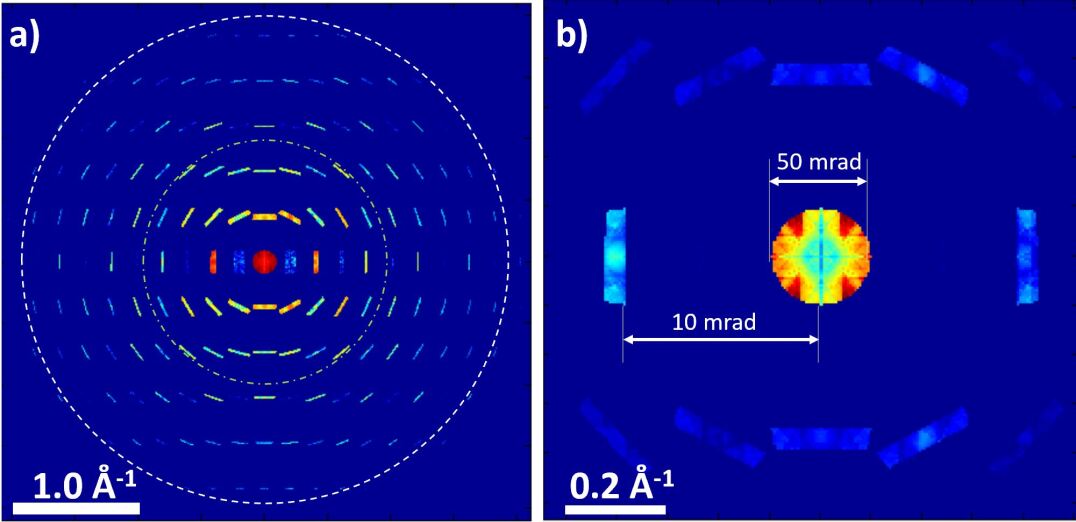
Figure 4: Simulated LARBED pattern of GaN (110) (simulation parameters in text). a) Complete diffraction pattern on a logarithmic scale: The largest g-vectors included as diffracted beams in this Bloch wave simulation have a reciprocal space length of 2Å^-1, as indicated by the white dashed circle. The green dash-dotted circle indicates the tilt range of the illumination during the LARBED simulation. b) Central part of the diffraction pattern on a linear scale: The geometry of the representation of the LARBD dataset is illustrated by highlighting that the scale of the LARBED discs is 10 times larger than that of the distance between discs (descan = 0.9 Koch (2011)).

Fig. 4 shows a simulated LARBED pattern of 10 nm thick GaN in the (110) zone axis. The accelerating voltage for this simulation was 200 kV and the maximum g-vector of reflections being simulated was 2Å^-1. The Bloch wave method was used for this simulation, where structure factors on reciprocal lattice points up to 4Å^-1 from the origin were included in the structure factor matrix. A total of 194 different structure factors (not counting $U_{0}$) were included in the calculation. The selection of beams that contributed to the diffraction pattern was carried out separately for each beam tilt, including only beams that were closer than 0.002Å^-1 to the Ewald sphere. This kept the number of beams in the simulation for each beam tilt relatively low but also leads to the sharp cutoff of diffraction discs, causing them to show mostly the Bragg lines (line in reciprocal space, along which the Bragg condition is very close to being matched for that reflection).

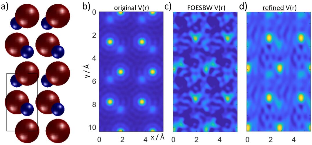
Figure 5: Reconstruction of the crystal potential from a simulated LARBED dataset: a) Structure of GaN in the (110) zone axis. 2 x 2 unit cells are being displayed, as is the case for Figs. b) - d). b) Original crystal potential simulated using independent atom scattering factors. c) Crystal potential resulting from all 194 structure factors that have been reconstructed using the first-order expansion stacked Bloch wave (FOESBW) approach described in this work. d) Bandwidth-limited potential resulting from a set of structure factors that was refined from the FOESBW-reconstruction using a simplex optimization of the full scattering matrix. The potential has been bandwidth limited to 2Å^-1, i.e. up to where reflection spots were simulated. All three potential maps are displayed using the same color map and -range.

Using the first order expansion of the Bloch wave formalism (eqn. (8)) in each layer, 45 layers were stacked, each having its independent set of structure factors. Having also analytical expressions for the gradient, gradient-based optimization was applied to find the structure factors in each of the layers. A constraint penalizing differences of corresponding structure factors in neighboring layers was added, initially with a very low weight, but increasing in weight, every time the cost function went below a given threshold. Since the diagonal entries of the first-order approximated scattering matrices given by eqn. (8) are actually zeroth order in structure factors (the 1st order vanishes), these values were also optimized for, even though they do not depend on any structure factor. Every 250 iterations corresponding elements of these diagonal entries were set to their average value.

Starting from a set of 194 structure factors which consisted of amplitudes fitted to the LARBED data using expression (6) and fully random structure factor phases, Fig. 5c shows a real-space representation of the average potential resulting from the first-order expansion stacked Bloch wave (FOESBW) optimization. Since the approximation to a full Bloch wave calculation is rather poor, the reconstruction is not expected to yield perfect agreement. However, in addition to the position of the Ga atoms, also the rough positions of the N atoms are visible, despite their more than 4 times lower Z-number. This set of complex-valued structure factors is then used as starting guess of a Nelder-Mead Simplex optimization using the Matlab function fminsearch. A bandwidth-limited version of the refined potential is shown in Fig. 5d. The bandwidth limiting seemed appropriate, because those structure factors that did not correspond to any diffracted intensity, but contributed only indirectly were only weakly determined due to the relatively low thickness.

Apart from a shift in unit cell origin which cannot be determined from the diffraction data, the agreement of the refined potential and the original one used as input for generating the simulated data is rather good. Note that the structure factors were not constrained in any way, neither by enforcing a real-valued (purely elastic) or positive potential, nor by assuming peakedness (atomicity). Since the imaginary part of the reconstructed potential consists of small numbers around zero, it is not shown here. By not assuming any atomicity in the reconstruction, this method is also applicable to highly beam-sensitive materials, where it may not be possible to collect diffraction data at sufficiently high resolution for atomicity-based phasing techniques to become applicable.

V Conclusion

In summary, two new methods for solving the inversion problem of dynamical scattering from LARBED data have been presented. Apart from the usually well-defined accelerating voltage the data required by the reconstruction may be directly obtained from the diffraction pattern alone. No assumptions are being made about the scattering potential within a single unit cell, making this method much more general than direct phasing methods applied to kinematical diffraction data, where a high degree of completeness and sufficient resolution for applying atomicity constraints are being required. The method uses dynamical scattering effects in the diffraction data to solve directly for the structure factor amplitudes and phases.

Although the application of this method to X-ray diffraction patterns is quite conceivable, it is expected that it’s main application will be in the field of structural electron crystallography. Simulated LARBED data of Si (110) and GaN (110) have been used to verify these methods.

References

- Vincent and Midgley (1994) R. Vincent and P. Midgley, Ultramicroscopy 53, 271 (1994).
- Moodie (1972) A. Moodie, Z. Naturforsch. 27, 437 (1972).
- Zuo and Spence (1991) J. M. Zuo and J. C. H. Spence, Ultramicroscopy 35, 185 (1991).
- Zuo et al. (1999) J. M. Zuo, M. Kim, M. O. Keeffe, and J. C. H. Spence, Nature 401, 49 (1999).
- Spence et al. (1990) J. C. H. Spence, B. Calef, and J. M. Zuo, Acta Cryst. A 46, 763 (1990).
- Spence (1998) J. C. H. Spence, Acta Cryst. A 54, 7 (1998).
- Allen et al. (1999) L. J. Allen, T. W. Josefsson, and H. Leeb, Acta Cryst. A 55, 105 (1999).
- Spence et al. (1999) J. C. H. Spence, B. Calef, and J. M. Zuo, Acta Cryst. A 55, 112 (1999).
- Allen et al. (1998) L. J. Allen, H. Leeb, and A. E. C. Spargo, Acta Cryst. A 54, 388 (1998).
- Allen et al. (2000) L. J. Allen, H. M. L. Faulkner, and H. Leeb, Acta Cryst. A 56, 119 (2000).
- Allen and Oxley (2001) L. J. Allen and M. Oxley, Ultramicroscopy 88, 195 (2001).
- Donatelli and Spence (2020) J. J. Donatelli and J. C. Spence, Phys. Rev. Lett. 125, 065502 (2020).
- Spence and Donatelli (2021) J. C. Spence and J. J. Donatelli, Ultramicroscopy 222, 113214 (2021).
- Chang (1982) S. L. Chang, Phys. Rev. Lett. 48, 163 (1982).
- Juretschke (1982) H. Juretschke, Phys. Rev. Lett. 48, 1487 (1982).
- Shen (1998) Q. Shen, Phys. Rev. Lett. 80, 3268 (1998).
- Saldin et al. (2002) D. Saldin, A. Seubert, and K. Heinz, Phys. Rev. Lett. 88, 115507 (2002).
- Allen et al. (2001) L. J. Allen, C. T. Koch, M. P. Oxley, and J. C. H. Spence, Acta Cryst. A 57, 473 (2001).
- Brown et al. (2018) H. G. Brown, Z. Chen, M. Weyland, C. Ophus, J. Ciston, L. Allen, and S. Findlay, Phys. Rev. Lett. 121, 266102 (2018).
- Koch and Spence (2003) C. T. Koch and J. C. H. Spence, J. Phys A: Math. and General 36, 803 (2003).
- Koch (2002) C. T. Koch, Ph.D. thesis, Arizona State University (2002).
- Koch (2011) C. Koch, Ultramicroscopy 111, 828 (2011).
- Wang et al. (2016) F. Wang, R. S. Pennington, and C. T. Koch, Phys. Rev. Lett. 117, 015501 (2016).
- Fujimoto (1959) F. Fujimoto, J. Phys. Soc, Japan 14, 1558 (1959).
- Humphreys (1979) C. J. Humphreys, Rep. Prog. Phys. 42, 1825 (1979).
- Cowley and Moodie (1957) J. M. Cowley and A. F. Moodie, Acta Cryst. 10, 609 (1957).
- Fujiwara (1959) K. Fujiwara, Journ. Phys. Soc. Japan 14, 1513 (1959).
- Sherali and Tuncbilek (1992) H. D. Sherali and C. H. Tuncbilek, Journal of Global Optimization 2, 101 (1992).
- Koch (2005) C. T. Koch, Acta Cryst. A 61, 231 (2005).
- Van den Broek et al. (2012) W. Van den Broek, A. Rosenauer, B. Goris, G. Martinez, S. Bals, S. Van Aert, and D. Van Dyck, Ultramicroscopy 116, 8 (2012).
- Van den Broek and Koch (2013) W. Van den Broek and C. T. Koch, Phys. Rev. B 87, 184108 (2013).
- Pennington et al. (2014) R. S. Pennington, F. Wang, and C. T. Koch, Ultramicroscopy 141, 32 (2014).
- Pennington and Koch (2015a) R. S. Pennington and C. T. Koch, Ultramicroscopy 155, 42 (2015a).
- Pennington and Koch (2015b) R. S. Pennington and C. T. Koch, Ultramicroscopy 148, 105 (2015b).
- Pennington et al. (2018) R. S. Pennington, C. Coll, S. Estrade, F. Peiro, and C. T. Koch, Phys. Rev. B 97, 024112 (2018).
- Igel and Hüsken (2000) C. Igel and M. Hüsken, in Proceedings of the Second International Symposium on Neural Computation, NC2000 (ICSC Academic Press, 2000), pp. 115–121.