A model-independent test for scale-dependent non-Gaussianities in the cosmic microwave background

Abstract

We present a model-independent method to test for scale-dependent non-Gaussianities in combination with scaling indices as test statistics. Therefore, surrogate data sets are generated, in which the power spectrum of the original data is preserved, while the higher order correlations are partly randomised by applying a scale-dependent shuffling procedure to the Fourier phases. We apply this method to the WMAP data of the cosmic microwave background (CMB) and find signatures for non-Gaussianities on large scales. Further tests are required to elucidate the origin of the detected anomalies.

Inflationary models of the very early universe have proved to be in very good agreement with the observations of the linear correlations of the cosmic microwave background (CMB). While the simplest, single field, slow-roll inflation Guth81 ; Linde82 ; Albrecht82 predicts that the temperature fluctuations of the CMB correspond to a (nearly) Gaussian, homogeneous and isotropic random field, more complex models may give rise to non-Gaussianity Linde97 ; Peebles97 ; Bernardeau02 ; Acquaviva03 . Models in which the Lagrangian is a general function of the inflaton and powers of its first derivative Armendariz99 ; Garriga99 can lead to scale-dependent non-Gaussianities, if the sound speed varies during inflation. Similarily, string theory models that give rise to large non-Gaussianity have a natural scale dependence Loverde08a . If the scale dependence of non-Gaussian signatures plays an important role in theory, the conventional (global) parametrisation of non-Gaussianity via $f_{NL}$ is no longer sufficient to describe the level of non-Gaussianity and to discriminate between different models. $f_{NL}$ must at least become scale dependent - if this parametrisation is sufficient at all. But first of all such scale-dependent signatures have to be identified.
Possible deviations from Gaussianity have been investigated in studies based on e.g. the WMAP data of the CMB (see Komatsu09a and references therein) and claims for the detection of non-Gaussianities and other anomalies (see e.g. Park04a ; Eriksen04a ; Hansen04 ; Eriksen05 ; Eriksen07 ; deoliveiracosta04 ; Raeth07 ; Mcewen08a ; Copi08a ) have been made. These studies have in common that the level of non-Gaussianity is assessed by comparing the results for the measured data with a set of simulated CMB-maps which were generated on the basis of the standard cosmological model and/or specific assumptions about the nature of the non-Gaussianities.
On the other hand, it is possible to develop model-independent tests for higher order correlations (HOCs) by applying the ideas of constrained randomisation Pompilio95a ; Raeth02 ; Raeth03 , which have been developed in the field of nonlinear time series analysis Theiler92 . The basic formalism is to compute statistics sensitive to HOCs for the original data set and for an ensemble of surrogate data sets, which mimic the linear properties of the original data. If the computed measure for the original data is significantly different from the values obtained for the set of surrogates, one can infer that the data contain HOCs.
Based on these ideas we present in this Letter a new method for generating surrogates allowing for probing scale-dependent non-Gaussianities.

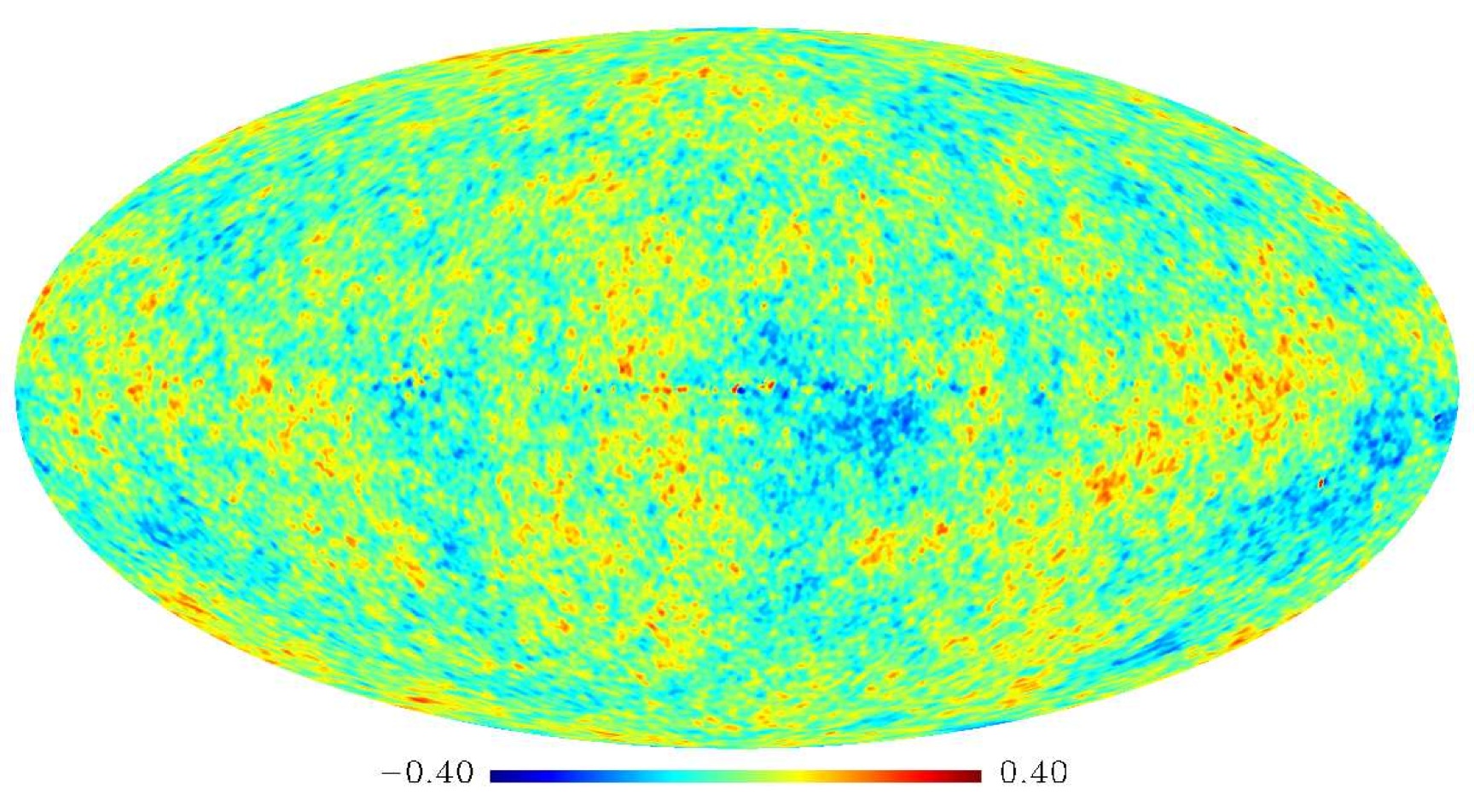
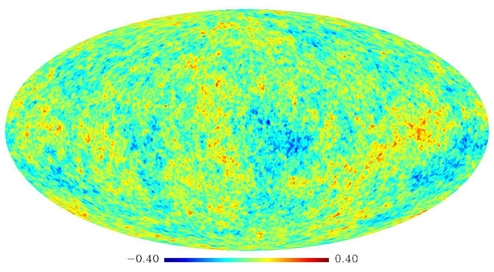
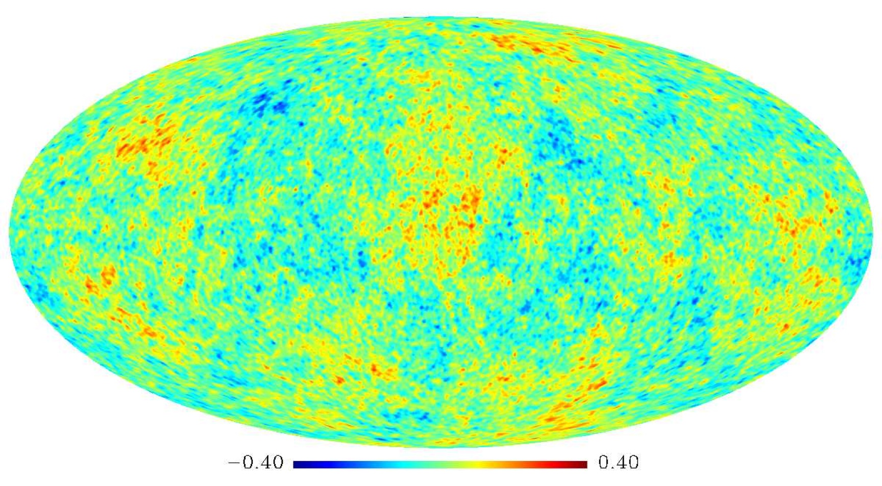
Figure 1: ILC map after remapping of the temperatures and phases (above). First order (middle) and respective second order surrogate (below) for $l_{cut}=20$. Note the resemblance of the first order surrogate with the ILC map at large scales

Our study is based on the WMAP data of the CMB. Since our method in its present form requires full sky coverage to ensure the orthogonality of the set of basis functions $Y_{lm}$ we used the five-year ”foreground-cleaned” Internal Linear Combination (ILC) map (WMAP5) Gold09a generated and provided by the WMAP-team. For comparison we also included the maps produced by Tegmark et al. Tegmark03 ; Deoliveiracosta06 , namely the three year cleaned map (TOHc3) and the Wiener-filtered cleaned map (TOHw3), which were generated pursuing a different approach for foreground cleaning. Since the Gaussianity of the temperature distribution and the randomness of the set of Fourier phases are a necessary prerequisite for the application of our method we performed the following preprocessing steps. First, the maps were remapped onto a Gaussian distribution in a rank-ordered way. By applying this remapping we automatically focus on HOCs induced by the spatial correlations in the data while excluding any effects coming from deviations of the temperature distribution from a Gaussian one.
To ensure the randomness of the set of Fourier phases we performed a rank-ordered remapping of the phases onto a set of uniformly distributed ones followed by an inverse Fourier transformation. These two preprocessing steps result in minimal changes to the ILC map (the maps remain highly correlated with cross-correlations $c>0.95$). The main effect is the removal of significant outliers in the temperature distribution. To test for scale-dependent non-Gaussianities in a model-independent way we propose the following two-step procedure. Without loss of generality we restrict the description of the method and all subsequent analyses to the case of non-Gaussianities on large scales. Consider a CMB map $T(\theta,\phi)$, where $T(\theta,\phi)$ is Gaussian distributed and calculate its Fourier transform. The complex valued Fourier coefficients $a_{lm}$, $a_{lm}=\int d\Omega_{n}T(n)Y^{*}_{lm}(n)$ can be written as $a_{lm}=|a_{lm}|e^{i\phi_{lm}}$ with $\phi_{lm}=\arctan\left(Im(a_{lm})/Re(a_{lm})\right)$. The linear or Gaussian properties of the underlying random field are contained in the absolute values $|a_{lm}|$, whereas all HOCs – if present – are encoded in the phases $\phi_{lm}$ and the correlations among them. First, we generate a first order surrogate map, in which any phase correlations for the scales, which are not of interest (here: the small scales), are randomised. This is achieved by a random shuffle of the phases $\phi_{lm}$ for $l>l_{cut},0<m\leq l$, where $l_{cut}=10,15,20,25,30$ in this Letter and by performing an inverse Fourier transformation (Fig. 1). Second, $N$ ($N=500$ for $l_{cut}=20$, $N=100$ otherwise) realisations of second order surrogate maps are generated for the first order surrogate map, in which the remaining phases $\phi_{lm}$ with $1<l\leq l_{cut},0<m\leq l$ are shuffled while the already randomised phases for the small scales are preserved. Fig. 1 shows a realisation of a second order surrogate map after inverse Fourier transformation. Note that the Gaussian properties of the remapped ILC map, which are given by $|a_{lm}|$, are exacly preserved in all surrogate maps. Finally, for calculating higher order statistics the maps were degraded to $N_{side}=256$ and residual monopole and dipole contributions were subtracted.

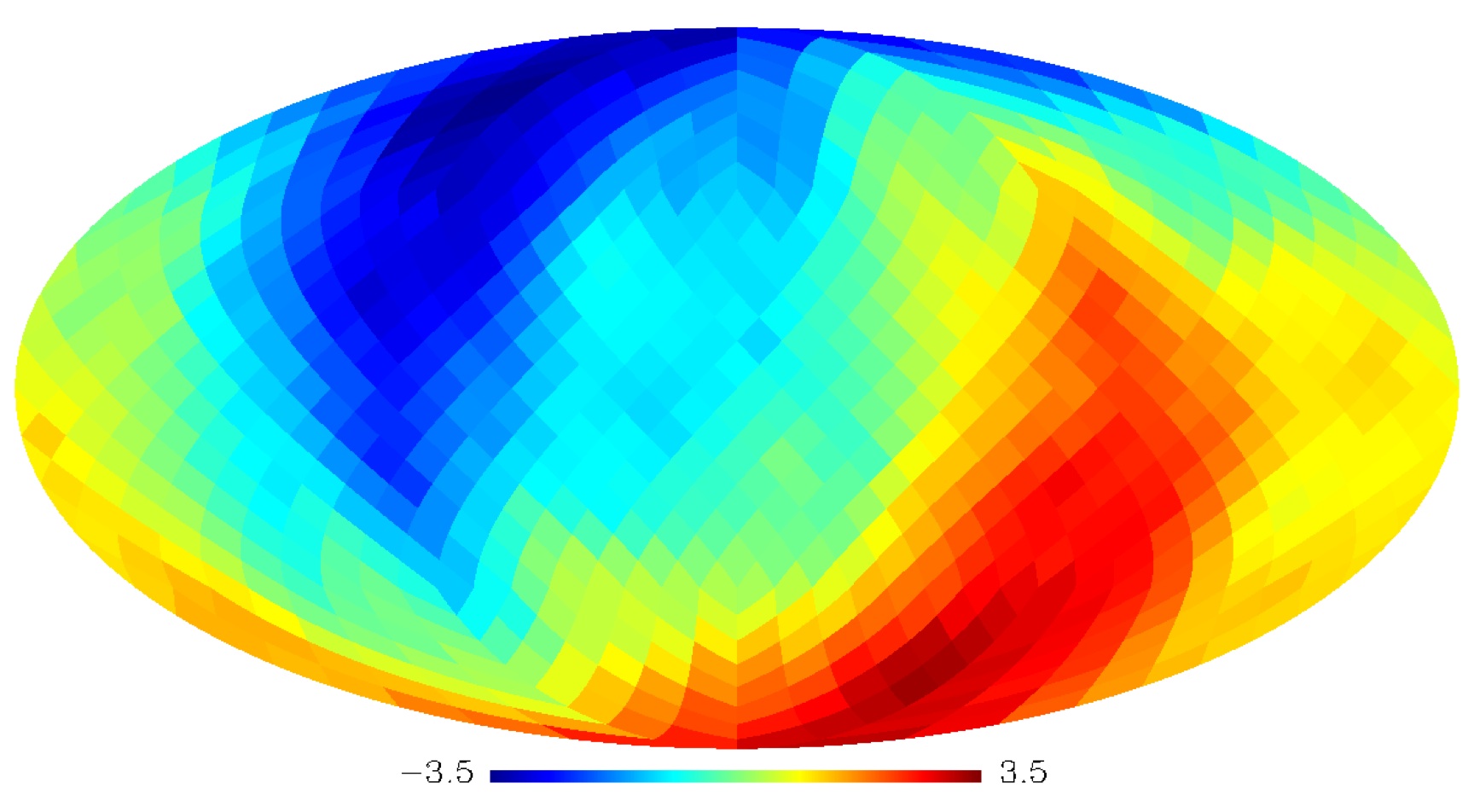
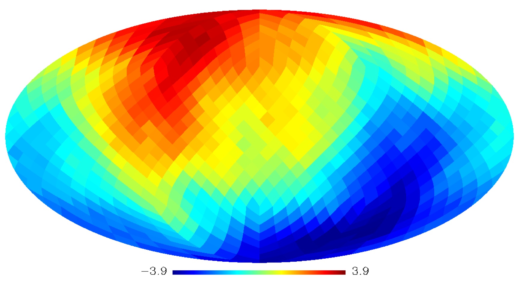
Figure 2: Deviation $S$ as derived from rotated upper hemispheres for $\sigma_{T}$ (above) and $\langle\alpha(r_{10})\rangle$ (below) for the WMAP5 map and $l_{cut}=20$. The z-axis of the respective rotated reference frame pierces the centre of the respective colour-coded pixel. $768$ rotated hemispheres, which correspond to number of coloured pixels, were considered. (For a more detailed description of this visualisation technique see e.g. Hansen04 ; Raeth07 ).

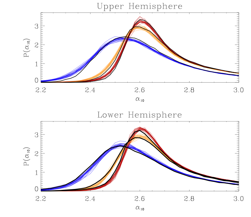
Figure 3: Probability density $P(\alpha(r_{10}))$ for the surrogates of the WMAP5 (blue), TOHw3 (yellow) and TOHc3 (red) map for the rotated upper and lower hemisphere and $l_{cut}=20$. The black lines denote the respective first order surrogate. The reference frame is chosen such that the difference $\Delta S=S_{up}-S_{low}$ between the upper and lower hemisphere becomes maximal for $\langle\alpha(r_{10})\rangle$ regarding the WMAP5 surrogates.

To compare the two classes of surrogates, we calculate local statistics in the spatial domain, namely scaling indices (SIM) as described in Räth et al. Raeth07 . In brief, scaling indices estimate local scaling properties of a point set $P$. The spherical CMB data can be represented as a three-dimensional point distribution $P=\vec{p_{i}}=(x_{i},y_{i},z_{i}),i=1,\ldots,N_{pixels}$ by transforming the temperature fluctuations into a radial jitter. For each point $\vec{p_{i}}$ the local weighted cumulative point distribution $\rho$ is calculated $\rho(\vec{p_{i}},r)=\sum_{j=1}^{N_{pixels}}e^{-(\frac{d_{ij}}{r})^{2}}\;,d_{ij}=\|\vec{p_{i}}-\vec{p_{j}}\|$. The weighted scaling indices $\alpha(\vec{p_{i}},r)$ are then obtained by calculating the logarithmic derivative of $\rho(\vec{p_{i}},r)$ with respect to $r$, $\alpha(\vec{p_{i}},r)=\frac{\partial\log\rho(\vec{p_{i}},r)}{\partial\log r}$. For each pixel we calculated scaling indices for ten different scales, $r_{1}=0.025$,…,$r_{10}=0.25$ in the notation of Raeth07 . For each scale we calculate the mean ($\langle\alpha\rangle$) and standard deviation ($\sigma_{\alpha}$) of the scaling indices $\alpha(\vec{p_{i}},r)$ derived from a set of pixels belonging to rotated hemispheres or the full sky. To investigate the correlations between the scaling indices and temperature fluctuations, we also considered the standard deviation ($\sigma_{T}$) for the mere temperature distribution of the respective sky regions.

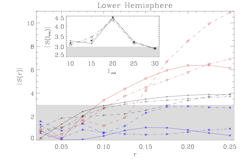
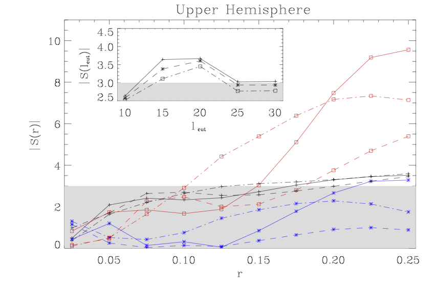
Figure 4: Deviations $|S(r)|$ for the rotated upper and lower hemisphere for $\langle\alpha\rangle$ (black), $\sigma_{\alpha}$ (blue) and a $\chi^{2}$-combination of $\langle\alpha\rangle$ and $\sigma_{\alpha}$ (red) ($l_{cut}=20$, $N=500$). The solid (dashed, dashed-dotted) lines denote the WMAP5 (TOHw3, TOHc3) map. The shaded region indicates the $3\sigma$ significance interval. The insets show the results for $\langle\alpha(r_{10})\rangle$, $\langle\alpha(r_{9})\rangle$ and $\langle\alpha(r_{8})\rangle$ (solid, dashed, dashed-dotted) as a function of $l_{cut}$ for the WMAP5 map (here: $N=100$).

Table 1: S/SL Upper Hemisphere

	WMAP5	TOHc3	TOHw3
	($S$/$SL$)	($S$/$SL$)	($S$/$SL$)
$\sigma_{T}$	-2.8/ 99.8	-3.0/$>$99.8	-2.9/  99.8
$\langle\alpha(r_{10})\rangle$	3.5 / $>$99.8	3.5 / $>$99.8	3.6 / $>$99.8
$\chi^{2}_{\langle\alpha\rangle}$	5.7 / 99.8	5.2 / 99.6	7.0 / $>$99.8
$\chi^{2}_{\sigma_{\alpha}}$	3.1 / 99.2	-0.7 / 74.4	2.1 / 95.4
$\chi^{2}_{\langle\alpha\rangle,\sigma_{\alpha}}$	6.1 / $>$ 99.8	3.6 / 99.0	6.4 / $>$ 99.8

Table 2: S/SL Lower Hemisphere

	WMAP5	TOHc3	TOHw3
	($S$/$SL$)	($S$/$SL$)	($S$/$SL$)
$\sigma_{T}$	2.7/99.8	2.9/$>$99.8	2.8/99.8
$\langle\alpha(r_{10})\rangle$	-3.9 / $>$99.8	-3.9 / $>$99.8	-3.7/$>$99.8
$\chi^{2}_{\langle\alpha\rangle}$	7.9 /$>$99.8	5.4/99.8	7.3/$>$99.8
$\chi^{2}_{\sigma_{\alpha}}$	-0.7 / 76.4	4.4 / 99.6	-0.6/67.0
$\chi^{2}_{\langle\alpha\rangle,\sigma_{\alpha}}$	5.8 / 99.8	6.3 /$>$99.8	5.2/$>$99.8

The differences of the two classes of surrogates are quantified by the $\sigma$-normalised deviation $S(Y)=(Y_{surro1}-\langle Y_{surro2}\rangle)/\sigma_{Y_{surro2}}$, $Y=\sigma_{T}$,$\langle\alpha\rangle$,$\sigma_{\alpha}$,$\chi^{2}$ (surro1: first order surrogate, surro2: second order surrogate) and the significance levels $SL=1-p$, where $p$ is the fraction of second order surrogates, which have a higher (lower) $Y$ than the first order surrogate. $\chi^{2}$ denotes diagonal $\chi^{2}$-statistics, which we obtain by combining $\langle\alpha\rangle$,$\sigma_{\alpha}$ for a given scale $r_{i}$, i.e. $\chi^{2}(r_{i})=\sum_{j=1}^{2}\left[\frac{X_{j}(r_{i})-\langle X_{j}(r_{i})\rangle}{\sigma_{X_{j}(r_{i})}}\right]^{2}\;,$ with $X_{1}=\langle\alpha\rangle,X_{2}=\sigma_{\alpha}$ and $\langle X_{j}\rangle$,$\sigma_{X_{j}}$ derived from the $N$ realisations of second order surrogates. As scale-independent measure we also consider $\chi^{2}$ as obtained by summing over the scales ($N_{r}=10$), $\chi^{2}=\sum_{i=1}^{N_{r}}\sum_{j=j_{1}}^{j_{2}}\left[\frac{X_{j}(r_{i})-\langle X_{j}(r_{i})\rangle}{\sigma_{X_{j}(r_{i})}}\right]^{2}\;,$ for one single measure ($j_{1}=1,j_{2}=1$; $j_{1}=2,j_{2}=2$) and the two measures ($j_{1}=1,j_{2}=2$). Fig. 2 shows $S(\sigma_{T})$ and $S(\langle\alpha(r_{10})\rangle)$ derived from pixels belonging to the respective upper hemispheres for $768$ rotated reference frames. Statistically significant signatures for non-Gaussianity and ecliptic hemispherical asymmetries become immediately obvious, whereby these signatures can solely be induced by large scale HOCs. Although $S(\sigma_{T})$ and $S(\langle\alpha(r_{10})\rangle)$ are spatially highly (anti-)correlated ($c=-0.95$), the two effects are nevertheless complementary to each other in the sense that a systematically lower/higher $\sigma_{T}$ would lead to a lower/higher $\langle\alpha(r_{10})\rangle$ and not to the observed higher/lower value for the first order surrogate map. These systematically shifted scaling indices are a generic feature present in all three maps (Fig. 3). Although the probability densities $P(\alpha(r_{10}))$ are different due to the smoothing or Wiener-filtering for the three maps, the shifts of the first order surrogate relative to its second order surrogates can be found in all three cases. We also cross-correlated the deviation maps shown in Fig. 2 derived from the three input maps and always obtained $c\geq 0.98$ for the correlation coefficient. These systematic deviations lead to significant detections of non-Gaussianities which are shown in Fig. 4 and summarised for $l_{cut}=20$ in Tables 1-2. The most significant and most stable results are found for $\langle\alpha\rangle$ at larger radii, where for all three maps none of the $500$ second order surrogates had a higher (upper hemisphere) or lower (lower hemisphere) value than the respective first order surrogate, leading to a significance level $SL>99.8$ % for $\langle\alpha(r_{10})\rangle$. Also the combined measure $\chi_{\langle\alpha\rangle}^{2}$ yields deviations $S$ ranging from $5.2$ up to $7.9$, which represent one of the most significant detection of non-Gaussianity in the WMAP data to date. We estimated how varying $l_{cut}$ values affect the results and found that both the non-Gaussianities and asymmetries are detected for all considered $l_{cut}$, where the highest deviations are obtained for $l_{cut}=20$. Although $S$ becomes considerably smaller for $l_{cut}=10$, we can still detect the non-Gaussianities with $SL>99.0$ %, which is larger than the results reported in Chiang07 ($SL=95$ %), where also $l_{cut}=10$ was used. We perfomed the same analyses for the coadded WMAP foreground template maps and for simulations using the best fit $\Lambda$CDM power spectrum and WMAP-like noise and beam properties. We found in none of these cases significant signatures as reported above. Details about these studies are deferred to a longer forthcoming publication.
In conclusion, we demonstrated the feasibility to generate new classes of surrogate data sets preserving the power spectrum and partly the information contained in the Fourier phases, while all other HOCs are randomised. We found significant evidence for both asymmetries and non-Gaussianities on large scales in the WMAP data of the CMB using scaling indices as test statistics. The novel statistical test involving new classes of surrogates allows for an unambigous relation of the signatures identified in real space with scale-dependent HOCs, which are encoded in the respective Fourier phase correlations. Our results, which are consistent with previous findings Park04a ; Eriksen04a ; Hansen04 ; Eriksen05 ; Eriksen07 ; Chiang07 ; Raeth07 but also extend to smaller scales than those reported in deoliveiracosta04 ($l_{cut}=3$) , Chiang07 $(l_{cut}=10)$ and Copi08a ($l_{cut}\leq 3$), point towards a violation of statistical isotropy and Gaussianity. Such features would disfavour canonical single-field slow-roll inflation – unless there is some undiscovered systematic error in the collection or reduction of the CMB data or yet unknown foreground contributions. Thus, at this stage it is too early to claim the detected HOCs as cosmological and further tests are required to elucidate the true origin of the detected anomalies. Their existence in the three maps might, however, be suggestive.
In either case the proposed statistical method offers an efficient tool to develop model-independent tests for scale-dependent non-Gaussianities. Due to the generality of this technique it can be applied to any signal, for which the analysis of scale-dependent HOCs is of interest.
Many of the results in this paper have been obtained using HEALPix Gorski05 . We acknowledge the use of LAMBDA. Support for LAMBDA is provided by the NASA Office of Space Science.

References

- (1) A. H. Guth, Phys. Rev. D 23, 347 (1981).
- (2) A. D. Linde, Phys. Lett. B 108, 389 (1982).
- (3) A. Albrecht and P. J. Steinhardt, Phys. Rev. Lett. 48, 1220 (1982).
- (4) A. D. Linde, V. Mukhanov, Phys. Rev. D 56, 535 (1997).
- (5) P. J. E. Peebles, Astrophys. J. Lett. 483, 1 (1997).
- (6) F. Bernardeau and J.-P. Uzan, Phys. Rev. D 66, 103506 (2002).
- (7) V. Acquaviva et al., Nucl. Phys. B 667, 119 (2003).
- (8) C. Armendariz-Picon, T. Damour and V. Mukhanov, Physics Letters B 458, 209 (1999).
- (9) J. Garriga and V. Mukhanov, Physics Letters B 458, 219 (1999).
- (10) M. Lo Verde et al., Journal of Cosmology and Astro-Particle Physics 4, 14 (2008).
- (11) E. Komatsu et al., Astrophys. J. Suppl. Ser. 180, 330 (2009).
- (12) C.-G. Park, Mon. Not. R. Astron. Soc. 349, 313 (2004).
- (13) H. K. Eriksen et al., Astrophys. J. 612, 64 (2004).
- (14) F. K. Hansen, A. J. Banday and K. M. Górski, Mon. Not. R. Astron. Soc. 354, 641 (2004).
- (15) H. K. Eriksen et al., Astrophys. J. 622, 58 (2005).
- (16) H. K. Eriksen et al., Astrophys. J. Lett. 660, 81 (2007).
- (17) A. de Oliveira-Costa et al., Phys. Rev. D 69, 063516 (2004).
- (18) C. Räth, P. Schuecker and A. J. Banday, Mon. Not. R. Astron. Soc. 380, 466 (2007).
- (19) J. D. McEwen et al., Mon. Not. R. Astron. Soc. 388, 659 (2008).
- (20) C. J. Copi et al., ArXiv e-prints 808 (2008), 0808.3767.
- (21) M. P. Pompilio et al., Astrophys. J. 449, 1 (1995).
- (22) C. Räth et al., Mon. Not. R. Astron. Soc. 337, 413 (2002).
- (23) C. Räth and P. Schuecker, Mon. Not. R. Astron. Soc. 344, 115 (2003).
- (24) J. Theiler et al., Physica D 58, 77 (1992).
- (25) B. Gold et al., Astrophys. J. Suppl. Ser. 180, 265 (2009).
- (26) M. Tegmark, A. de Oliveira-Costa and A. J. Hamilton, Phys. Rev. D 68, 123523 (2003).
- (27) A. de Oliveira-Costa and M. Tegmark, Phys. Rev. D 74, 023005 (2006).
- (28) L.-Y. Chiang, P. D. Naselsky and P. Coles, Astrophys. J. 664, 8 (2007).
- (29) K. M. Górski et al., Astrophys. J. 622, 759 (2005).