Quark mass dependence of thermal excitations in QCD in one-loop approximation

Abstract

A comprehensive determination of the quark mass dependence in the dispersion relations of thermal excitations of gluons and quarks in non-Abelian gauge theory (QCD) is presented for the one-loop approximation in Feynman gauge. Larger values of the coupling are admitted, and the gauge dependence is discussed. In a Dyson-Schwinger type approach, the effect of higher orders is estimated for asymptotic thermal masses.

1 Introduction

The broad research programme of ultra-relativistic heavy-ion collisions aims at investigating a new state of deconfined strongly interacting matter. Experimentally, the hints for such a state, dubbed quark-gluon plasma, have been accumulated in investigations at CERN-SPS [1] and further consolidated at BNL-RHIC [2]. While early ideas have been guided by asymptotic freedom considering the quark-gluon plasma as an ensemble of weakly interacting quarks and gluons, the paradigm has changed now to a strongly coupled quark-gluon plasma [3], as enforced by the success of hydrodynamical concepts which point to an extremely fast thermalization [3] and an exceedingly low viscosity [4, 5].

Parallel to the intense experimental efforts, which will soon proceed to a new era at CERN-LHC, much progress has been achieved on the theoretical side. In particular, first-principle (lattice) QCD calculations, directly based on numerical evaluations of the QCD partition function, are progressing and deliver information on the equation of state and related thermodynamic quantities such as susceptibilities etc. [6]. While final results on bulk properties of deconfined strongly interacting matter at finite temperatures seem to be achievable in the near future, the microscopic nature – with respect to the excitations in the considered medium – received less attention hitherto.

In fact, a variety of phenomenological approaches basing on different microscopic pictures account fairly well for the bulk information obtained in lattice QCD. For instance, various effective quasi-particle models [7, 8, 9, 10, 11, 12, 13] rely on qualitatively formulated / postulated excitations in the quark-gluon medium in order to achieve a parametrization of the equation of state adjusted to lattice QCD results. Certain symmetries of QCD are the basis of PNJL models (cf. [14]) which also need adjustments to lattice QCD data. Other approaches assume that the QGP may be described by a classical non-relativistic plasma of colour charges with Coulomb interaction [15] for temperatures $T_{c}<T<3T_{c}$, where $T_{c}$ is the pseudo-critical or deconfinement temperature. Analytical attempts to derive the equation of state from QCD by perturbative means [16] are in agreement with the non-perturbative lattice QCD results for temperatures $T>3T_{c}$. These approaches also provide some legitimation for a quasi-particle picture that goes beyond strict perturbation theory [17].

At asymptotically large temperatures suitable techniques like dimensional reduction [19] bring further insight into the structure of the theory and are applicable, e.g., to the physics of the early universe. (Here, at temperatures 1 - 100 GeV, the heavy quark sector becomes important [18].) Strict perturbative expansions have been pushed to order $g^{6}\ln g$ (see [19, 20] and references therein) and slightly beyond [18], where $g$ is the strong coupling. The successful hard thermal loop/hard dense loop (HTL/HDL) resummation scheme [21] employs HTL self-energies, which correspond to the high temperature/density limit of one-loop self-energies, thus, setting all quark masses to zero. The systematics of one-loop and HTL self-energies, as well as the corresponding dispersion relations were studied in [22] for zero quark masses. Further steps towards going beyond the one-loop approximations have been attempted in [23], where a Dyson-Schwinger scheme is set up in ladder approximation and in the chiral limit focussing on the fermion spectral function.

It is the temperature region $T_{c}-5T_{c}$ which is of utmost relevance for heavy-ion collisions. Here, the information on the excitation spectrum of deconfined matter is fairly scarce. In [24], the poles of quark and gluon propagators in Coulomb gauge have been analyzed with the result that they may be parametrized by an energy ($\omega$) - momentum ($k$) relation $\omega^{2}=k^{2}+m_{q,g}^{2}$ with $m_{q,g}/T=\xi_{q,g}$ and $\xi_{q,g}$ ranging from 1.2 till 3.9 depending on parton species and temperature. Karsch and Kitazawa [25] analyzed, in quenched approximation and in Landau gauge, spectral properties of quarks at $1.5T_{c}$ and $3T_{c}$ and at zero momentum as a function of the bare quark mass $m$. An important result of these investigations is the confirmation of a mass gap $m_{q}=\xi_{q}(T)T$ with a weak temperature dependence in the function $\xi_{q}(T)$. Another important result in [25] concerns the quark mass dependence of pole positions and residues of the quark propagator, which was found to be qualitatively different from the expected perturbative pattern.

For the latter one, systematic investigations are hardly found in the literature. The thermal self-energies of gluons (e.g. [26]) and quarks (e.g. [27]) have been calculated for massive quarks. Fermion mass effects on the dispersion relations have been studied by several authors [27, 28, 29, 30] with the restriction to the long-wavelength limit of the dispersion relations or to small (soft) masses $m\leq gT$ or $m\leq g\mu$, where $\mu$ is the quark chemical potential.

A more detailed investigation of the general mass dependence in the dispersion relations is desired, e.g., to uncover effects of masses $m\sim{\cal O}(T)$, as employed in lattice QCD calculations [31]. A deeper understanding of the impact of heavy quark masses on the equation of state of strongly interacting matter relevant for the early universe is also of interest.

The chiral extrapolation, and thus the quark mass dependence, is an important issue not only in thermo-field theory. Also in low energy effective field theories, such as chiral perturbation theory, the chiral extrapolation of quantities like the nucleon mass is of great interest [32]. In hot QCD it is particularly challenging as lattice QCD evaluations have been performed often for nonphysically heavy quarks due to technical limitations. Apart from the necessary continuum extrapolation, the extrapolation to physical quark masses is an inevitable step towards obtaining useable results.

Given this motivation, we present here the systematics of the quark mass dependence of quasi-particle dispersion relations in hot one-loop QCD. We mention as further motivation that in a series of papers [7, 9, 10] the successful description of lattice QCD results on bulk properties of strongly interacting matter was demonstrated within a phenomenological quasi-particle model employing approximate one-loop dispersion relations for quarks and gluons. The model [7, 9, 10, 11] goes beyond perturbation theory by using an effective coupling rather than the strong coupling. This motivates us not to restrict ourselves to the weak coupling regime.

Our paper is organized as follows. In section 2, we present numerical results of the thermal part of gluon one-loop self-energies and related quantities, in particular the dispersion relations which offer a glimpse on the relevant excitations. Section 3 illuminates the same quantities but now for quarks. Section 4 is devoted to the gauge dependence of our results. For this purpose, we contrast our results with calculations in Coulomb gauge. Of course, there are regions in parameter space where our results coincide with the HTL approximation, which has been proved to be gauge independent in [33]. The summary can be found in section 5. Appendix A lists necessary relations for the chiral expansion of the asymptotic thermal masses and Appendix B contains the decomposition of the quark propagator with non-zero quark mass into different physical excitations according to the spinor structure of the propagator. In Appendix C, figures for quantifying the self-energies are collected. In Appendix D, we present an asymptotic Dyson-Schwinger approach to estimate higher order contributions to the mass dependence of the asymptotic thermal masses in the case of Abelian gauge theory.

2 One-loop gluon excitations

In the following, we consider the quark masses as well as the coupling $g$ as external parameters. Our results are presented for two-flavor QCD ($N_{f}=2$) with one independent quark mass parameter to limit the dimensions of parameter space. However, a generalization to cover a hierarchy of different quark masses is straightforward. We focus on the thermal parts of the self-energies at zero chemical potential (quark–anti-quark symmetric hot QCD medium), having in mind, however, the remarks given in [28].

2.1 Gluon self-energy

The gluon one-loop self-energy may be decomposed as

$$\Pi_{\mu\nu,ab}^{g}(K)=\Pi_{\mu\nu,ab}^{YM}(K)+\sum_{q}\Pi_{\mu\nu,ab}^{q}(K)$$ (1)

with Lorentz indices $\mu,\nu$ and colour indices $a,b$ of the adjoint representation of the gauge group. The contributions of gluon loop ($3g$), gluon tadpole ($4g$), and ghost loop ($ghost$) are grouped in the Yang-Mills contribution ”$YM$”. The quark loops are labelled by ”$q$” and the sum runs over all quark flavors included. They read as functions of the four-momentum $K$ of the considered gluon

$$\Pi{{}^{YM}_{\mu\nu,ab}}(K) = \frac{1}{2}T\sum_{\omega_{n}}\int\frac{d^{3}p}{(2\pi)^{3}}\mbox{tr}\big{[}\Gamma_{\mu\alpha\beta}^{3g}{\cal D}_{\alpha\sigma}(P)\Gamma_{\tau\sigma\nu}^{3g}{\cal D}_{\tau\beta}(Q)\big{]}_{ab}$$ (2)

$$+ \frac{1}{2}T\sum_{\omega_{n}}\int\frac{d^{3}p}{(2\pi)^{3}}\mbox{tr}\big{[}\Gamma_{\mu\alpha\beta\nu}^{4g}{\cal D}_{\alpha\beta}(P)\big{]}_{ab}$$

$$+ T\sum_{\omega_{n}}\int\frac{d^{3}p}{(2\pi)^{3}}\mbox{tr}\big{[}\Gamma_{\mu}^{ghost}G(P)\Gamma_{\nu}^{ghost}G(Q)\big{]}_{ab}\,\,,$$

$$\Pi{{}^{q}_{\mu\nu,ab}}(K) = -T\sum_{\omega_{n}}\int\frac{d^{3}p}{(2\pi)^{3}}\mbox{tr}\big{[}\Gamma_{\mu}^{q}{\cal S}(Q)\Gamma_{\nu}^{q}{\cal S}(P)\big{]}_{ab}.$$ (3)

In the above expressions the fermion (F) and boson (B) propagators are the bare propagators ${\cal S}={\cal S}_{0}(K)=(m-/K)\Delta_{F}(K)$ and ${\cal D}_{\mu\nu}=({\cal D}_{0})_{\mu\nu}=\delta_{\mu\nu}\Delta_{B}(K)$ in Feynman gauge suppressing the explicit colour indices for notational convenience, with the thermal propagators $\Delta_{F}(K)=(\omega_{n}^{2}+k^{2}+m^{2})^{-1}$ and $\Delta_{B}(K)=(\omega_{n}^{2}+k^{2})^{-1}$ with Matsubara frequencies $\omega_{n}=2n\pi T$ and $\omega_{n}=(2n+1)\pi T$ for bosonic and fermionic degrees of freedom, respectively. The trace ”tr” has to be taken over spinor and colour indices and $P$ and $Q=P-K$ are the internal loop four-momenta. For the expressions of the various vertices $\Gamma$ we refer to standard textbooks on thermo-field theory, e.g. [34].

The tensor $\Pi_{\mu\nu}^{g}$ consists of two independent scalar functions according to

$$\Pi_{\mu\nu}^{g}={\mathfrak{P}}_{\mu\nu}^{T}\Pi_{T}^{g}+{\mathfrak{P}}_{\mu\nu}^{L}\Pi_{L}^{g},$$ (4)

where the utilized four-transverse projectors ($K^{\mu}{\mathfrak{P}}_{\mu\nu}^{T,L}=0$) are given by

$${\mathfrak{P}}_{\mu\nu}^{T}=g_{\mu\nu}-\frac{K_{\mu}K_{\nu}}{K^{2}}+\frac{{\mathfrak{P}}_{\mu\nu}^{L}}{N^{2}},\qquad{\mathfrak{P}}_{\mu\nu}^{L}=-N_{\mu}N_{\nu}$$ (5)

with $N_{\mu}=\left(K_{\mu}(Ku)-u_{\mu}K^{2}\right)\left((Ku)^{2}-K^{2}\right)^{-1}$ and $K^{\mu}N_{\mu}=0$. The superscripts $T$ and $L$ indicate that the tensors ${\mathfrak{P}}^{T}_{\mu\nu}$ and ${\mathfrak{P}}^{L}_{\mu\nu}$ project on subspaces transverse and longitudinal to the three-momentum ${\bf k}$, respectively. After performing the summation over the Matsubara frequencies, integrating over the angular part of $d^{3}p$ and analytically continuing into Minkowski space-time one obtains for the individual scalar functions [26]

$$\Pi_{L}^{YM}(\omega,k) = -\frac{C_{A}g^{2}}{\pi^{2}}\int\limits_{0}^{\infty}dpp\,n_{B}(p)\left[1-\frac{2k^{2}-\omega^{2}-4p^{2}}{8pk}\ln{\cal A}_{g}+\frac{\omega}{2k}\ln{\cal B}_{g}\right],$$ (6)

$$\Pi_{T}^{YM}(\omega,k) = \frac{C_{A}g^{2}}{2\pi^{2}}\int\limits_{0}^{\infty}dpp\,n_{B}(p)\left[1+\frac{\omega^{2}}{k^{2}}-\frac{3k^{2}+\omega^{2}+4p^{2}}{8pk^{3}}(k^{2}-\omega^{2})\ln{\cal A}_{g}\right.$$ (7)

$$\left.-\frac{\omega}{2k^{3}}(k^{2}-\omega^{2})\ln{\cal B}_{g}\ \right],$$

$$\Pi_{L}^{q}(\omega,k) = -\frac{2C_{2}g^{2}}{\pi^{2}}\int\limits_{0}^{\infty}dp\,\frac{p^{2}}{\epsilon_{\bf p}}n_{F}(\epsilon_{\bf p})\left[1-\frac{k^{2}-\omega^{2}-4\epsilon_{\bf p}^{2}}{8kp}\ln{\cal A}_{f}-\frac{\omega\epsilon_{\bf p}}{2kp}\ln{\cal B}_{f}\right],$$ (8)

$$\Pi_{T}^{q}(\omega,k) = \frac{C_{2}g^{2}}{\pi^{2}}\int\limits_{0}^{\infty}dp\,\frac{p^{2}}{\epsilon_{\bf p}}n_{F}(\epsilon_{\bf p})\left[1+\frac{\omega^{2}}{k^{2}}-\frac{k^{4}-\omega^{4}-4\epsilon_{\bf p}^{2}\omega^{2}+4p^{2}k^{2}}{8pk^{3}}\ln{\cal A}_{f}\right.$$ (9)

$$+\left.\frac{\omega\epsilon_{\bf p}}{2pk^{3}}(k^{2}-\omega^{2})\ln{\cal B}_{f}\right]$$

with

$${\cal A}_{g} = \frac{(k^{2}-\omega^{2}+2pk)^{2}-4p^{2}\omega^{2}}{(k^{2}-\omega^{2}-2pk)^{2}-4p^{2}\omega^{2}},\qquad{\cal B}_{g}=\frac{(k^{2}-\omega^{2})^{2}-4p^{2}(k+\omega)^{2}}{(k^{2}-\omega^{2})^{2}-4p^{2}(k-\omega)^{2}},$$ (10)

$${\cal A}_{f} = \frac{(k^{2}-\omega^{2}+2pk)^{2}-4\omega^{2}\epsilon_{\bf p}^{2}}{(k^{2}-\omega^{2}-2pk)^{2}-4\omega^{2}\epsilon_{\bf p}^{2}},\qquad{\cal B}_{f}=\frac{(k^{2}-\omega^{2})^{2}-4(pk+\omega\epsilon_{\bf p})^{2}}{(k^{2}-\omega^{2})^{2}-4(pk-\omega\epsilon_{\bf p})^{2}}$$ (11)

and $\epsilon_{\bf p}=\sqrt{p^{2}+m^{2}}$. $K\sim(\omega,{\bf k})$ consists of the two components $\omega=K\cdot u$ and $\bf k$ with $|{\bf k}|=k=\sqrt{(K\cdot u)^{2}-K^{2}}$ in the thermal medium with four-velocity $u_{\mu}$. $n_{F,B}$ are the standard Fermi and Bose distribution functions and the gauge group factors are $C_{A}=N_{c}$, $C_{2}=1/2$ for a $\mbox{SU}(N_{c})$ gauge group with $N_{c}=3$ for QCD.

\psfrag{0}{\tiny$0$}\psfrag{1}{\tiny$1$}\psfrag{2}{\tiny$2$}\psfrag{3}{\tiny$3$}\psfrag{4}{\tiny$4$}\psfrag{5}{\tiny$5$}\psfrag{6}{\tiny$6$}\psfrag{7}{\tiny$7$}\psfrag{8}{\tiny$8$}\psfrag{9}{\tiny$9$}\psfrag{0.0}{\tiny$0.0$}\psfrag{0.5}{\tiny$0.5$}\psfrag{1.0}{\tiny$1.0$}\psfrag{1.5}{\tiny$1.5$}\psfrag{2.0}{\tiny$2.0$}\psfrag{2.5}{\tiny$2.5$}\psfrag{3.0}{\tiny$3.0$}\psfrag{3.5}{\tiny$3.5$}\psfrag{4.0}{\tiny$4.0$}\psfrag{4.5}{\tiny$4.5$}\psfrag{5.0}{\tiny$5.0$}\psfrag{5.5}{\tiny$5.5$}\psfrag{6.0}{\tiny$6.0$}\psfrag{6.5}{\tiny$6.5$}\psfrag{7.0}{\tiny$7.0$}\psfrag{0.10}{\tiny$0.10$}\psfrag{0.12}{\tiny$0.12$}\psfrag{0.14}{\tiny$0.14$}\psfrag{0.16}{\tiny$0.16$}\psfrag{0.18}{\tiny$0.18$}\psfrag{0.20}{\tiny$0.20$}\psfrag{0.2}{\tiny$0.2$}\psfrag{0.4}{\tiny$0.4$}\psfrag{0.6}{\tiny$0.6$}\psfrag{0.8}{\tiny$0.8$}\psfrag{g = 0.3}{\tiny$g=0.3$}\psfrag{g = 1.0}{\tiny$g=1.0$}\psfrag{g = 3.0}{\tiny$g=3.0$}\psfrag{xlog-2}{\tiny$10^{-2}$}\psfrag{xlog-1}{\tiny$10^{-1}$}\psfrag{xlog0}{\tiny$1$}\psfrag{xlog1}{\tiny$10$}\psfrag{xlabel}{ \small$\omega^{2}/g^{2}T^{2}$}\psfrag{ylabel}{ \small${\rm Re\ }\Pi_{T}^{q}/g^{2}T^{2}$}\psfrag{label1}{}\psfrag{label2}{}\psfrag{label3}{$\omega^{2}-k^{2}$}\includegraphics[scale={0.32},angle={-90}]{figures/figure1.eps}

Figure 1: The scaled real part of the quark loop contribution to the transverse gluon self-energy according to (9) as a function of the scaled energy for $N_{f}=2$ degenerate quark flavors with mass $m/T=0$ (blue short-dashed curve), $0.5$ (red solid curve) and $0.7$ (green long-dashed curve). The kinky structure at $\omega=\sqrt{k^{2}+4m^{2}}$ is clearly visible. The black dotted line represents $\omega^{2}-k^{2}$. Thus, the intersection with the self-energy function would represent the sole solution of the dispersion relation if there were no other contributions. The curves are for $g=1$ and $k=gT$.

For illustration, figure 1 exhibits the real part of $\Pi_{T}^{q}$ as a function of $\omega$ for three different values of the quark mass at fixed $k$. The real parts of the quark loop contributions $\Pi_{T,L}^{q}$ develop a non-analytical (continuous but not continuously differentiable) behaviour at the threshold $\omega^{2}=k^{2}+4m^{2}$ for the production of a real quark–anti-quark pair. This behaviour is, however, related to the imaginary part of $\Pi_{T}^{q}$, which is also non-zero above the threshold $\omega^{2}>k^{2}+4m^{2}$. The imaginary parts in such one-loop calculations are known to have no direct physical meaning since the quasi-particle damping rates (related to the widths of quasi-particle peaks in the spectral function) turn out to be gauge dependent, both, in magnitude and even in sign. Braaten and Pisarski [21] pointed out the necessity of resumming diagrams of higher-loop order (HTL resummation) to get a definite result. However, the excitation energies of the quasi-particles considered in this paper are rather independent of the imaginary parts.

With the replacements $g\to e$, $m\to m_{e}$, $C_{A}\to 0$, $C_{2}\to 1$ and $N_{f}\to 1$ the quantities $\Pi_{T,L}^{q}$ would represent the thermal transverse and longitudinal one-loop photon self-energy contributions in a hot Abelian (QED) plasma, respectively. Such plasmas are presently of interest [35, 36], as their production under laboratory conditions seems feasible with high-intensity lasers. The temperature of such a plasma is expected to be in the range of $T\sim 1\ldots 10$ MeV while the electron mass $m_{e}\approx 511$ keV sets an additional energy scale. Thus, in this temperature region, in particular for lower temperatures, the ratio $m_{e}/T$ is not small, which might lead to modifications in certain plasma properties as compared to the ultra-relativistic case. Consequently, a non-negligible electron mass is expected to influence physical observables such as production rates of pions and muons [35] and of photons [37].

2.2 Gluon dispersion relations

The dressed gluon propagator may be decomposed as

$${\cal D}_{\mu\nu}^{ab}(K)=\delta^{ab}\left({\mathfrak{P}}_{\mu\nu}^{T}\Delta_{T}+{\mathfrak{P}}_{\mu\nu}^{L}\frac{k^{4}}{K^{4}}\Delta_{L}+\rho\frac{K_{\mu}K_{\nu}}{K^{4}}\right)$$ (12)

with gauge fixing parameter $\rho=1$ in Feynman gauge and the projectors ${\mathfrak{P}}_{\mu\nu}^{T,L}$ are defined in the explanation below equation (4). The transverse and longitudinal propagator parts are related to the corresponding self-energies by Dyson’s equation via

$$\Delta_{T}=\frac{1}{K^{2}-\Pi^{g}_{T}(\omega,k)}, \Delta_{L}=\frac{1}{k^{2}-\Pi^{g}_{L}(\omega,k)}$$ (13)

with $\Pi^{g}_{T,L}=\Pi_{T,L}^{YM}+\sum_{q}\Pi_{T,L}^{q}$.

The gluon one-loop self-energies possess in general real and imaginary contributions. Here, we are interested in the dispersion relations of gluonic quasi-particle excitations with negligible damping rates, which are characterized by

$${{\rm Re\ }}\Big{(}\Delta_{T,L}^{-1}\Big{)}=0.$$ (14)

The gluon excitation energies, which are the real solutions of (14), may be represented by $\omega^{2}_{T,L}=k^{2}+{\cal G}_{T,L}m_{g}^{2}$ with $m_{g}^{2}=\frac{1}{6}g^{2}T^{2}(N_{c}+N_{f}/2)$. The contribution $m_{g}^{2}{\cal G}_{T,L}$ to the quasi-particle excitation energy encodes the effects of the thermal medium and represents a thermal mass. Therefore, the light cone is given by the planes ${\cal G}_{T,L}\equiv 0$ in this representation. For the transverse gluon excitation one can write ${\cal G}_{T}\equiv{\rm Re\ }\Pi_{T}(\omega(k),k,m)/m_{g}^{2}$ and for longitudinal gluons (plasmons) one finds ${\cal G}_{L}\equiv K^{2}{\rm Re\ }\Pi_{L}(\omega(k),k,m)/(k^{2}m_{g}^{2})$. In the presently considered case, the parameter space is three-dimensional for fixed temperature: The functions ${\cal G}_{T,L}$ depend on $m$, $g$ and $k$. Note that the $g$ dependence cannot be scaled out, unlike in the HTL approximation. We are interested in the regions $m\sim T$ and $k\sim T$. The first range is determined by the lattice calculations [31] which employ ”lattice quark masses” $m\propto T$; the interesting range is extended till the chiral limit $m=0$. The second range is determined by the observation [7] that thermal excitations with $k\sim T$ essentially contribute to thermodynamic quantities. A survey of these functions is exhibited in figure 2 for $N_{f}=2$ quarks of mass $m$.

The overall observation is, that the thermal contribution to the transverse gluon mode stays above the light cone in the whole parameter range, whereas it drops and rapidly approaches the light cone for the longitudinal mode at sufficiently large momenta, independent of $g$ and $m$. Both, ${\cal G}_{T}$ and ${\cal G}_{L}$, are monotonically decreasing with increasing mass $m$, indicating that heavy quarks, compared to massless quarks, contribute not as much to the thermal mass of the gluon. The $m$ dependence is, though, rather weak because the thermal masses are dominated by the strong gluonic self-interaction. For the transverse mode, the function ${\cal G}_{T}$ approaches unity in the limit $k\to\infty$ and $m\to 0$, exposing that $m_{g}$ is the asymptotic mass, indeed. We emphasize the strong $g$ dependence when considering the region $g\sim 1$, see figure 2. (Note that $g=1$ corresponds to $\alpha_{S}\approx 0.08$, whereas $g=0.3$ translates to $\alpha_{S}\approx{1}/{137}$ and $g=3$ means $\alpha_{S}\approx 0.72$). Clearly, for large values of $g$, higher order contributions are expected to become important.

Such 3D plots are useful for surveys, however, cuts allow for a better quantitative representation of results. Corresponding figures are relegated to Appendix C (cf. figures 5 and 6).

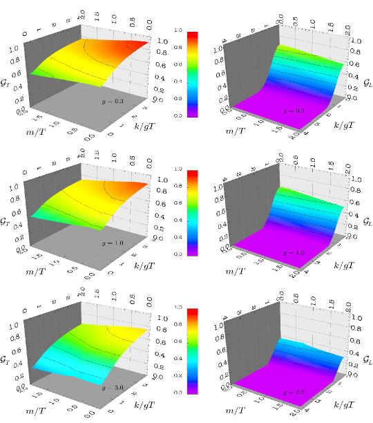
Figure 2: Transverse (left) and longitudinal (right) gluon dispersion relations represented as ${{\cal G}_{T,L}}=({\omega^{2}_{T,L}-k^{2}})/{m_{g}^{2}}$ as functions of scaled momentum and scaled quark mass for $g=0.3,\,1.0,\,3.0$ from top to bottom. For a better presentation, the transverse and longitudinal quantities are considered from different perspectives. Faint isolines are given at ${\cal G}_{T,L}=0.1,0.2,\ldots,0.9.$

2.3 Gluon plasma frequency and asymptotic behaviour

It is instructive to study some special limiting cases of the dispersion relations, where the mass dependence of the thermal mass part of the excitation energies can be given explicitly by analytical formulae. The gluon plasma frequency is defined as the long wavelength limit of the gluon dispersion relation $\displaystyle\omega_{pl}=\lim_{k\to 0}\omega_{T,L}(k)$, yielding after some calculations

$$\omega_{pl}^{2} = \frac{1}{9}g^{2}T^{2}\left(N_{c}+C_{2}\sum_{q}^{N_{f}}{\cal J}\left(\frac{m_{q}}{T}\right)\right)\,\chi(g,\{m_{q}\}),$$ (15)

$${\cal J}(x) = \frac{18}{\pi^{2}}x^{2}\int\limits_{0}^{\infty}d\xi\,\frac{\xi^{2}}{\sqrt{1+\xi^{2}}}\left(1-\frac{\xi^{2}}{3(1+\xi^{2})}\right)\frac{1}{1+\exp({x\sqrt{1+\xi^{2}}})}$$ (16)

with the same value for the transverse and longitudinal polarizations, giving rise to a mass gap, i.e. $\omega(k\to 0)>0$. In general, $\chi(g,\{m_{q}\})$ depends on a vector $\{m_{q}\}$ with components $m_{q}$. The function $\chi(g,m)=\chi(g,\{m,m\})$, depicted in the left panel of figure 3 for one independent mass $m=m_{q}$ and $N_{f}=2$, is implicitly defined by (15) with the numerically determined value of $\omega_{pl}=\omega(k\to 0)$ on the l.h.s. It approaches unity for small values of $g$ in agreement with the HTL result. At large values of the coupling $g$, $\chi(g,m)$ rapidly drops, making the plasma frequency soft. In addition, $\chi(g,m)$ is almost independent of $m$ in the range of interest. From this follows that the mass dependence of the plasma frequency is essentially contained in the function ${\cal J}(m/T)$, which is depicted in figure 3, right panel. For large values of $m/T$, ${\cal J}(m/T)$ behaves like $\exp(-m/T)$ indicating the decoupling of the heavy quark sector from the thermal bath, while for decreasing values of $m/T$, ${\cal J}(m/T)$ approaches unity with ${m/T\to 0}$. Thus, in the limit $g\to 0$ and $m\to 0$ or $T\to\infty$, equation (15) gives the usual HTL gluon plasma frequency $\hat{\omega}_{pl}^{2}=\frac{1}{9}g^{2}T^{2}(N_{c}+C_{2}N_{f})$.

\psfrag{0}{\tiny$0$}\psfrag{1}{\tiny$1$}\psfrag{2}{\tiny$2$}\psfrag{3}{\tiny$3$}\psfrag{4}{\tiny$4$}\psfrag{5}{\tiny$5$}\psfrag{6}{\tiny$6$}\psfrag{7}{\tiny$7$}\psfrag{8}{\tiny$8$}\psfrag{9}{\tiny$9$}\psfrag{0.0}{\tiny$0.0$}\psfrag{0.5}{\tiny$0.5$}\psfrag{1.0}{\tiny$1.0$}\psfrag{1.5}{\tiny$1.5$}\psfrag{2.0}{\tiny$2.0$}\psfrag{2.5}{\tiny$2.5$}\psfrag{3.0}{\tiny$3.0$}\psfrag{3.5}{\tiny$3.5$}\psfrag{4.0}{\tiny$4.0$}\psfrag{4.5}{\tiny$4.5$}\psfrag{5.0}{\tiny$5.0$}\psfrag{5.5}{\tiny$5.5$}\psfrag{6.0}{\tiny$6.0$}\psfrag{6.5}{\tiny$6.5$}\psfrag{7.0}{\tiny$7.0$}\psfrag{0.10}{\tiny$0.10$}\psfrag{0.12}{\tiny$0.12$}\psfrag{0.14}{\tiny$0.14$}\psfrag{0.16}{\tiny$0.16$}\psfrag{0.18}{\tiny$0.18$}\psfrag{0.20}{\tiny$0.20$}\psfrag{0.2}{\tiny$0.2$}\psfrag{0.4}{\tiny$0.4$}\psfrag{0.6}{\tiny$0.6$}\psfrag{0.8}{\tiny$0.8$}\psfrag{g = 0.3}{\tiny$g=0.3$}\psfrag{g = 1.0}{\tiny$g=1.0$}\psfrag{g = 3.0}{\tiny$g=3.0$}\psfrag{xlog-2}{\tiny$10^{-2}$}\psfrag{xlog-1}{\tiny$10^{-1}$}\psfrag{xlog0}{\tiny$1$}\psfrag{xlog1}{\tiny$10$}\psfrag{xlabel}{\small$g$}\psfrag{ylabel}{\small$\chi(g,m)$}\psfrag{xlabelmass}{\hskip 7.11317pt\small$m/T$}\psfrag{ylabelmass}{\hskip 7.11317pt\small$\cal I,J$}\psfrag{labelI}{\tiny$\cal I$}\psfrag{labelJ}{\tiny$\cal J$}\includegraphics[scale={0.32},angle={-90}]{figures/figure3a.eps}

\psfrag{0}{\tiny$0$}\psfrag{1}{\tiny$1$}\psfrag{2}{\tiny$2$}\psfrag{3}{\tiny$3$}\psfrag{4}{\tiny$4$}\psfrag{5}{\tiny$5$}\psfrag{6}{\tiny$6$}\psfrag{7}{\tiny$7$}\psfrag{8}{\tiny$8$}\psfrag{9}{\tiny$9$}\psfrag{0.0}{\tiny$0.0$}\psfrag{0.5}{\tiny$0.5$}\psfrag{1.0}{\tiny$1.0$}\psfrag{1.5}{\tiny$1.5$}\psfrag{2.0}{\tiny$2.0$}\psfrag{2.5}{\tiny$2.5$}\psfrag{3.0}{\tiny$3.0$}\psfrag{3.5}{\tiny$3.5$}\psfrag{4.0}{\tiny$4.0$}\psfrag{4.5}{\tiny$4.5$}\psfrag{5.0}{\tiny$5.0$}\psfrag{5.5}{\tiny$5.5$}\psfrag{6.0}{\tiny$6.0$}\psfrag{6.5}{\tiny$6.5$}\psfrag{7.0}{\tiny$7.0$}\psfrag{0.10}{\tiny$0.10$}\psfrag{0.12}{\tiny$0.12$}\psfrag{0.14}{\tiny$0.14$}\psfrag{0.16}{\tiny$0.16$}\psfrag{0.18}{\tiny$0.18$}\psfrag{0.20}{\tiny$0.20$}\psfrag{0.2}{\tiny$0.2$}\psfrag{0.4}{\tiny$0.4$}\psfrag{0.6}{\tiny$0.6$}\psfrag{0.8}{\tiny$0.8$}\psfrag{g = 0.3}{\tiny$g=0.3$}\psfrag{g = 1.0}{\tiny$g=1.0$}\psfrag{g = 3.0}{\tiny$g=3.0$}\psfrag{xlog-2}{\tiny$10^{-2}$}\psfrag{xlog-1}{\tiny$10^{-1}$}\psfrag{xlog0}{\tiny$1$}\psfrag{xlog1}{\tiny$10$}\psfrag{xlabel}{\small$g$}\psfrag{ylabel}{\small$\chi(g,m)$}\psfrag{xlabelmass}{\hskip 7.11317pt\small$m/T$}\psfrag{ylabelmass}{\hskip 7.11317pt\small$\cal I,J$}\psfrag{labelI}{\tiny$\cal I$}\psfrag{labelJ}{\tiny$\cal J$}\includegraphics[scale={0.32},angle={-90}]{figures/figure3b.eps}

Figure 3: Left panel: Function $\chi(g,m)$ defined in (15), showing the non-trivial dependence of the gluon plasma frequency as a function of the coupling $g$. On the displayed scale, curves for $0\leq m/T\leq 2$ are on top of each other. Right panel: Functions ${\cal J}$ (dashed curve) and ${\cal I}$ (solid curve) as defined in (16) and (18), respectively.

In the asymptotic region, $k\rightarrow\infty$, the transverse gluon dispersion relation is given by the gauge invariant result $\omega^{2}=k^{2}+m_{\infty}^{2}$ with the asymptotic gluon mass

$$m_{\infty}^{2} = {\rm Re\ }\Pi_{T}^{g}(k,k)=\frac{1}{6}g^{2}T^{2}\left(N_{c}+C_{2}\sum_{q}^{N_{f}}{\cal I}\left(\frac{m_{q}}{T}\right)\right),$$ (17)

$${\cal I}(x) = \frac{12}{\pi^{2}}x^{2}\int\limits_{0}^{\infty}d\xi\,\frac{\xi^{2}}{\sqrt{1+\xi^{2}}}\frac{1}{1+\exp({x\sqrt{1+\xi^{2}}})}.$$ (18)

The function $\cal I$ is depicted in the right panel of figure 3. The power expansion for small values of $m/T$ (cf. Appendix A) reads

$${\cal I}\left(\frac{m}{T}\right)=1+\alpha_{2}\left(\frac{m}{T}\right)^{2}+\alpha_{L}\left(\frac{m}{T}\right)^{2}\ln\left(\frac{m}{T}\right)^{2}+\alpha_{4}\left(\frac{m}{T}\right)^{4}+\sum_{j=3}^{\infty}\alpha_{2j}\left(\frac{m}{T}\right)^{2j}$$ (19)

with coefficients $\alpha_{n}$ listed in table 1 relegated to Appendix A. This expansion of $\cal I$ is convergent in the region $m/T<\pi$. Note the term $\propto\alpha_{L}$ resembling chiral logarithms. Equations (17) and (18) highlight an important feature occurring in the gluon sector, here, for the example of asymptotic dispersion relations. As the quark loop contribution is added to the gluon and ghost loops, the mass dependence is not so striking in the range of $m$ we are interested in. For instance, for $N_{f}=2$ the term in brackets in (17) varies in the range between $4$ and $3$ while going from $m=0$ to $m\to\infty$, evidencing the dominance of the strong non-Abelian self-coupling compared to the quark loop contributions in the thermal masses. In a QED plasma there is, of course, a much stronger dependence of the thermal photon mass on the electron mass $m_{e}$.

The heavy-quark expansion for $m/T\gg 1$ yields, as evident from (40) in Appendix A,

$${\cal I}\left(\frac{m}{T}\right)\simeq\frac{12}{\pi^{2}}\sqrt{\frac{\pi m}{2T}}\rme^{-\frac{m}{T}}.$$ (20)

As ${\cal I}(m/T)$ becomes exponentially small for large values of $m/T$, the heavy quarks decouple also in the asymptotic momentum region from the thermal bath (i.e., they are exponentially suppressed).

3 One-loop quark excitations

3.1 Quark self-energy

The one-loop quark self-energy represented in the imaginary time formalism reads

$$\Sigma(K) = -T\sum_{n}\int\frac{d^{3}p}{(2\pi)^{3}}\big{[}\Gamma^{q}_{\mu}{\cal S}(Q)\Gamma_{\nu}^{q}{\cal D}_{\mu\nu}\big{]}$$ (21)

with loop momenta $P$ and $Q=K-P$. The general structure of the self-energy reads

$$\Sigma=a\,/K+b\,/u-c=\gamma_{0}\tilde{b}(\omega,k)-{\boldsymbol{\gamma}}{\bf k}a(\omega,k)-c(\omega,k)$$ (22)

with the medium 4-velocity $u_{\mu}$ and $\tilde{b}=\omega a+b$. After performing the Matsubara sum and continuing into Minkowski space-time one finds for the three independent self-energy functions

$$a(\omega,k) = \frac{g^{2}C_{F}}{2\pi^{2}k^{2}}\int\limits_{0}^{\infty}dp\,\left[\frac{p^{2}}{\epsilon_{\bf p}}n_{F}(\epsilon_{\bf p})\left(1+\frac{h_{F}}{8kp}\ln(a_{F}^{+}a_{F}^{-})+\frac{d_{F}}{8kp}\ln\frac{a_{F}^{+}}{a_{F}^{-}}\right)\right.$$ (23)

$$+pn_{B}(p)\left.\left(1+\frac{h_{B}}{8kp}\ln(a_{B}^{+}a_{B}^{-})+\frac{d_{B}}{8kp}\ln\frac{a_{B}^{+}}{a_{B}^{-}}-\frac{k}{4p}\ln(a_{B}^{+}a_{B}^{-})\right)\right],$$

$$\tilde{b}(\omega,k) = \frac{g^{2}C_{F}}{8\pi^{2}k}\int\limits_{0}^{\infty}dp\,p\left[n_{F}(\epsilon_{\bf p})\ln\frac{a_{F}^{+}}{a_{F}^{-}}+n_{B}(p)\left(\ln\frac{a_{B}^{+}}{a_{B}^{-}}-\frac{\omega}{p}\ln(a_{B}^{+}a_{B}^{-})\right)\right],$$ (24)

$$c(\omega,k) = m\frac{g^{2}C_{F}}{4\pi^{2}k}\int\limits_{0}^{\infty}dp\,p\left[\frac{n_{F}(\epsilon_{\bf p})}{\epsilon_{\bf p}}\ln(a_{F}^{+}a_{F}^{-})-\frac{n_{B}(p)}{p}\ln(a_{B}^{+}a_{B}^{-})\right]$$ (25)

with $C_{F}=(N_{c}^{2}-1)/(2N_{c})$, and the abbreviations read

$$a_{F}^{\pm} = \frac{k^{2}-m^{2}-\omega^{2}\pm 2\epsilon_{\bf p}\omega-2pk}{k^{2}-m^{2}-\omega^{2}\pm 2\epsilon_{\bf p}\omega+2pk},$$ (26)

$$a_{B}^{\pm} = \frac{k^{2}+m^{2}-\omega^{2}\pm 2p\omega-2pk}{k^{2}+m^{2}-\omega^{2}\pm 2p\omega+2pk},$$ (27)

$$h_{F} = k^{2}-m^{2}-\omega^{2},\quad d_{F}=2\epsilon_{\bf p}\omega,$$ (28)

$$h_{B} = k^{2}+m^{2}-\omega^{2},\quad d_{B}=2p\omega\,.$$ (29)

3.2 Quark dispersion relations

The dispersion relations are determined by the poles of the resummed quark propagator ${\cal S}$, given by the Dyson equation ${\cal S}^{-1}={\cal S}_{0}^{-1}+\Sigma$, leading to

$${\cal S}^{-1}=\gamma_{0}(\omega+\tilde{b})-{\boldsymbol{\gamma}}{\bf k}(1+a)-(m+c).$$ (30)

With the definitions of projectors relegated to Appendix B, this can be rewritten yielding

$${\cal S}=\frac{{\mathfrak{P}}^{+}_{{\bf k},m}\gamma_{0}}{r(n\omega-{\cal E})}+\frac{{\mathfrak{P}}^{-}_{{\bf k},m}\gamma_{0}}{r(n\omega+{\cal E})}.$$ (31)

The quark (plasmino) dispersion relation is obtained as the positive energy solution of $n\omega_{q}-{\cal E}=0$ ($n\omega_{p}+{\cal E}=0$). The dispersion relations for the quasi-particles may be parametrized as $\omega_{q}^{2}=k^{2}+m^{2}+m_{f}^{2}{\cal F}_{q}$ and $\omega_{p}^{2}=k^{2}+m_{f}^{2}{\cal F}_{p}$ for quarks and plasminos, respectively. The functions ${\cal F}_{p,q}$,which non-trivially depend on $k$ and $m$, encode the effects on the excitations induced by the thermal medium with temperature $T$. For fixed $k$ and $m$ these functions multiplied by $m_{f}^{2}$ serve as effective thermal mass parameters. ${\cal F}_{q}=0$ accounts for a simple on-shell dispersion relation, while ${\cal F}_{p}=0$ represents the light cone. The quantity $m_{f}^{2}=\frac{1}{8}C_{F}g^{2}T^{2}$ is the usual HTL quark plasma frequency, setting a typical energy scale in these studies [34].

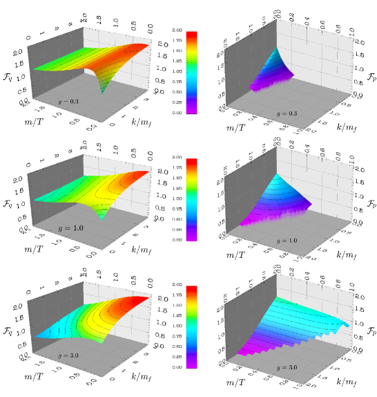
Figure 4: Quark (left) and plasmino (right) dispersion relations represented as ${\cal F}_{q}=(\omega_{q}^{2}-k^{2}-m^{2})/m_{f}^{2}$ for regular quark excitations and ${\cal F}_{p}=({\omega^{2}_{p}-k^{2}})/m_{f}^{2}$ for plasmino excitations as functions of scaled momentum and scaled quark mass for $g=0.3,\,1.0,\,3.0$ from top to bottom. For a better representation, the regular quark and the plasmino quantities are considered from different perspectives. Faint isolines are for ${\cal F}_{q,p}=0.1,0.2,\ldots 1.9$. The representation of ${\cal F}_{p}$ in the right panel ends where numerically no real solutions of the dispersion relations can be found.

A survey of this representation of the dispersion relations is exhibited in figure 4, where the temperature dependent parts ${\cal F}_{q}$ and ${\cal F}_{p}$ for regular quark and collective plasmino excitations are shown in the left and right columns, respectively. Again, different cuts allowing for a better quantitative representation are relegated to Appendix C (cf. figures 7 and 8). Further examinations of the one-loop self-energies show that these exhibit non-zero imaginary parts, both, below and above the light cone which are particularly large below the light cone.

Considering, instead, $\omega_{p}^{2}=k^{2}+m_{f}^{2}{\cal F}_{p}$ as a function of $k^{2}$, the plasmino branch exhibits a local minimum which, however, vanishes for $m>gT$. This local minimum gives rise to van Hove singularities in certain emission rates [38].

In addition, for any value of $m>0$, the collective branch completely disappears from the spectrum for momenta larger than a certain critical one. Furthermore, the plasmino branch lies energetically below the regular quark excitation branch $\omega_{q}^{2}$ (Surprisingly, the lattice QCD calculations [25] show an opposite order at $k=0$).

As mentioned above, with some replacements (here, one has to use $C_{F}\to 1$ in addition) the electron excitations in an electron-positron QED plasma are also described. Particularly interesting would be an experimental verification of the purely collective plasmino excitations.

3.3 Quark plasma frequency and asymptotic behaviour

For vanishing momenta $k\to 0$, the plasma frequencies for quarks ($+$) and plasminos ($-$) $\omega_{\pm}=\omega(k\to 0)$ are implicitly given by

$$\omega_{\pm}\mp m+\left.\Big{(}\tilde{b}\mp c\Big{)}\right|_{k\to 0}=0,$$ (32)

where we used $\left.(ka)\right|_{k\to 0}=0$ due to rotational invariance. The long-wavelength limit of the quark dispersion relation is therefore independent of the function $a$. An explicit calculation of the various limits yields the implicit equation

$$0 = \omega_{\pm}\mp m+\frac{g^{2}C_{F}}{2\pi^{2}}\int\limits_{0}^{\infty}\frac{dp\,p}{z_{\pm}^{2}-p^{2}}\left[n_{F}(\epsilon_{\bf p})\frac{p\epsilon_{\bf p}}{\omega_{\pm}^{2}}(\omega_{\pm}\mp m)\right.$$ (33)

$$\hskip 113.81102pt\left.+\frac{n_{B}(p)}{\omega_{\pm}}\Big{(}(p^{2}\mp mz_{\pm})+z_{\pm}(\omega_{\pm}\mp m)\Big{)}\right]\,$$

with $z_{\pm}=(m^{2}-\omega_{\pm}^{2})/2\omega_{\pm}$. The splitting of the two branches is of order $m$; in the chiral limit, $m\to 0$, both branches meet at $k=0$. In the limit $g\ll 1$ and $m\lesssim gT$, one recovers a formula given by Pisarski [30]

$$\omega_{\pm}=\frac{1}{2}\left(\sqrt{m^{2}+4m_{f}^{2}}\pm m\right),$$ (34)

and the difference of the plasma frequencies of quarks and plasminos becomes $\omega_{+}-\,\omega_{-}=m$. Thus, the regular quark has a higher excitation energy than the plasmino. In the limit $m=0$ the high temperature result $\omega_{\pm}=m_{f}$ is obtained.

In the asymptotic region, the momentum $k$ is the largest scale, allowing for some approximations to obtain an explicit analytic expression for the asymptotic dispersion relation of the regular quark excitation. In this case, the equation $n\omega-{\cal E}=0$ can be transformed to yield

$$\omega^{2}=k^{2}+m^{2}+2\left.\Big{(}k^{2}\,a+k\,\tilde{b}\Big{)}\right|_{k\to\infty},$$ (35)

which is completely independent of the self-energy function $c$. The asymptotic quark dispersion relation can then be written as

$$\omega^{2}=k^{2}+m^{2}+2M_{+}^{2},\quad M_{+}^{2}=\frac{1}{3}m_{f}^{2}\left({\cal I}\left(\frac{m}{T}\right)+2\right)$$ (36)

with the integral $\cal I$ given in (18) and the same expansion as in (19). For $m\to 0$, one finds $M_{+}^{2}\to m_{f}^{2}$.

4 Gauge dependence

As the HTL approximation has been proved to be gauge independent [33], one may look for regions in parameter space where the self-energies in one-loop approximation coincide with HTL results. The real parts of the HTL and one-loop self-energies coincide for small values of $\omega$ and $k$, of course, but for larger values of $\omega$ and/or k both may deviate noticeably in general. However, near the light cone, i.e. for $\omega\approx k$, they are approximately equal , and on the light cone, $\omega=k$, HTL and one-loop self-energies coincide, cf. [11, 39]. The self-energies slightly above the light-cone determine the excitation energies of the quasi-particles in a wide parameter range and are, therefore, relevant for the quasi-particle model [7, 9].

The gauge independence of the asymptotic gluon mass $m_{\infty}^{2}$ can be shown by noting that the transverse parts of the Yang-Mills contributions to the gluon self-energy at the light cone $\Pi_{T}^{YM}(k,k)$ are exactly the same in the one-loop and HTL approximations. Furthermore, the quark contribution $\Pi_{T}^{q}$ is inherently gauge independent at one-loop level. Hence, the asymptotic thermal gluon mass is a gauge invariant quantity.

To check further for the gauge dependence of the above one-loop results in Feynman gauge – here in particular we focus on the asymptotic mass of regular quarks – we compare them with explicit calculations in Coulomb gauge. For large momenta, the regular quark excitation energies in Feynman gauge ($\omega$) and Coulomb gauge ($\omega_{C}$) are related via

$$\omega_{C}^{2}(\omega,k) = \omega^{2}(\omega,k)+\Delta_{C}(\omega,k),$$ (37)

$$\Delta_{C}(\omega,k) = \frac{g^{2}C_{F}}{\pi^{2}}\int\limits_{0}^{\infty}dp\,\frac{p^{2}}{\epsilon_{\bf p}}n_{F}(\epsilon_{\bf p})\left(1-\frac{k^{2}+p^{2}}{4kp}\,\ln\frac{k^{2}+p^{2}+2kp}{k^{2}+p^{2}-2kp}\right),$$ (38)

with $\displaystyle\lim_{k\to\infty}\Delta_{C}(\omega,k)\to 0$, thus proving the coincidence of the dispersion relations in both gauges in the asymptotic region.

5 Summary

In summary, we survey the quark mass dependence of thermal one-loop self-energies and emerging dispersion relations of quarks and gluons in QCD in Feynman gauge. The motivation and the related focus of our presentation are given by upcoming lattice QCD results on spectral properties of quarks and gluons in a hot and deconfined medium and the need of chiral extrapolations in bulk properties of the quark-gluon plasma. While the results of [25] are at variance with the energetic ordering of quark and plasmino excitations from perturbative QCD, they otherwise confirm the existence of a mass gap of quarks in line with basic assumptions of the successful phenomenological quasi-particle model [7, 9]. The present analysis challenges the chiral extrapolation of the equation of state performed in [40], as the important term $\propto mM_{+}$ in the quark excitation dispersion relation is not supported by our one-loop results. This may be considered as further hint to strong non-perturbative effects in the quark-gluon plasma in a range accessible in present and future heavy-ion collisions. Indeed, the asymptotic Dyson-Schwinger type approach outlined in Appendix D, points to severe corrections to the one-loop results in the strong coupling regime for fermion masses of the order of the temperature. Progressing lattice QCD results are required to reveal the fundamental excitations of deconfined matter.

Appendix A Expansion of the function ${\mathcal{I}}$

To derive the expansion in (19) of the function ${\cal I}$ given in (18) we rewrite the expression using $(\epsilon_{\bf p}+1)^{-1}=\sum_{j=1}^{\infty}(-1)^{j+1}\rme^{-j\epsilon_{\bf p}}$ to

$${\cal I}(x)=\frac{12}{\pi^{2}T^{2}}\sum_{j=1}^{\infty}(-1)^{j+1}\int\limits_{0}^{\infty}dp\frac{p^{2}}{\epsilon_{\bf p}}\rme^{-j\epsilon_{\bf p}}$$ (39)

and obtain

$${\cal I}(x)=\frac{12}{\pi^{2}}\sum_{j=1}^{\infty}(-1)^{j+1}\frac{x}{j}K_{1}(jx)$$ (40)

with $x=m/T$. For small quark masses, $x\to 0$, one may represent $\cal I$ as

$${\cal I}(x)=\frac{1}{2\pi i}\frac{12}{\pi^{2}}\sum_{j=1}^{\infty}\int\limits_{c-i\infty}^{c+i\infty}ds\,(-1)^{j+1}j^{-s-1}\,x^{1-s}\,{\cal M}[K_{1};s]$$ (41)

with the Mellin transform

$${\cal M}[K_{1};s] = \int\limits_{0}^{\infty}dz\,z^{s-1}K_{1}(z)=2^{s-2}\,\Gamma\Big{(}\frac{s-1}{2}\Big{)}\,\Gamma\Big{(}\frac{s+1}{2}\Big{)}$$ (42)

of the first modified Bessel function of the second kind $K_{1}$.
Exploiting $\sum_{j=1}^{\infty}(-1)^{j+1}j^{-s-1}=\left(1-2^{-s}\right)\zeta(s+1),$ with the Riemann zeta function $\zeta$, we find as intermediate step

$${\cal I}(x)=\frac{12}{\pi^{2}}\frac{1}{2\pi i}\int\limits_{c-i\infty}^{c+i\infty}ds\,\frac{x^{1-s}}{2^{2-s}}\left(1-\frac{1}{2^{s}}\right)\zeta(s+1)\,\Gamma\Big{(}\frac{s-1}{2}\Big{)}\,\Gamma\Big{(}\frac{s+1}{2}\Big{)},$$ (43)

which can be evaluated with a suitable contour and appropriate $c$ [39] to yield

$${\cal I} = \sum_{i}\left.\mbox{Res}\,f(s)\right|_{s=s_{i}},$$ (44)

$$f(s) = \frac{6}{\pi^{2}}\,\frac{x^{1-s}}{2^{1-s}}\left(1-\frac{1}{2^{s}}\right)\zeta(s+1)\,\Gamma\Big{(}\frac{s-1}{2}\Big{)}\,\Gamma\Big{(}\frac{s+1}{2}\Big{)}.$$ (45)

Further evaluation leads to the series in (19) with coefficients given in table 1. Although the numerical value of the coefficients rapidly approaches zero, this expansion has a finite radius of convergence, which is

$$R^{2}=\lim_{n\to\infty}\left|\frac{\alpha_{n}}{\alpha_{n+2}}\right|=\pi^{2},\qquad\,n\geq 4\,.$$ (46)

Table 1: The coefficients of the chiral expansion in (19). $\gamma_{E}$ is the Euler-Mascheroni number and $\zeta$ stands for Riemann’s zeta function.

• coefficient	analytic expression	numerical value
  $\alpha_{2}$	$-\frac{3}{\pi^{2}}(\ln\pi+\frac{1}{2}-\gamma_{E})$	$\approx-0.32449$
  $\alpha_{L}$	$\frac{3}{2\pi^{2}}$	$\approx\hbox{\phantom{-}}0.15198$
  $\alpha_{4}$	$-\frac{21}{16\pi^{4}}\zeta(3)$	$\approx-1.619\cdot 10^{-2}$
  $\alpha_{6}$	$\frac{93}{128\pi^{6}}\zeta(5)$	$\approx\hbox{\phantom{-}}7.836\cdot 10^{-4}$
  $\alpha_{8}$	$-\frac{1905}{4096\pi^{8}}\zeta(7)$	$\approx-4.943\cdot 10^{-5}$
  $\alpha_{n}$	$(-1)^{\frac{n-2}{2}}\,\frac{24}{n}\,\frac{2^{n-1}-1}{(2\pi)^{n}}\,\frac{(n-3)!!}{(n-2)!!}\zeta(n-1)$
  	for $n=4,6,8,\ldots$

Appendix B Quark propagator

The explicit breaking of chiral symmetry drastically modifies the structure of the quark propagator compared to the usually treated case, where all current quark masses are set to zero. As a consequence, the usual projectors, which allow for a distinction of the different quasi-particle states, are not applicable. Thus, one has to examine in some detail the spinor structure of the propagator, which provides projectors to the relevant subspaces of the physical (quasi-particle) excitations. For the self-energy we employ the decomposition given in (22). Utilizing Dyson’s equation yields the general structure for the inverse quark propagator

$${\cal S}^{-1}=r\left(n\omega\gamma_{0}-{\boldsymbol{\gamma}}{\bf k}-{\cal M}\right)$$ (47)

with the three self-energy functions $r\equiv(1+a)$, $n\equiv 1+b/\omega r$ and ${\cal M}\equiv(m+c)/(1+a)$, depending on $\omega,|{\bf k}|$ and $m$. Although there is an explicit breaking of chiral symmetry due to the finite current quark masses, chiral symmetry is assumed not to be broken spontaneously at high temperature, thus, $\displaystyle\lim_{m\to 0}{\cal M}(\omega,k,m)=0$. In contrast to the vacuum, an additional function $n$ appears, which may be interpreted as an analogue to the refraction index in optics [41]. The appearance of this function is due to the breaking of Lorentz invariance by the term $\propto/u$ in (22).

The spinors $\psi$ representing the quasi-particle states are supposed to be solutions of the Dirac equation

$$(n\omega\gamma_{0}-{\boldsymbol{\gamma}}{\bf k}-{\cal M})\psi(k)=0.$$ (48)

Non-trivial solutions are found only for $n^{2}\omega^{2}={\cal E}^{2}$ with ${\cal E}=+\sqrt{k^{2}+{\cal M}^{2}}$. This is an implicit equation for the excitation energies $\omega$ of the system, leading to $\omega=\pm{\cal E}/n$. A Hamiltonian may be defined by

$${\cal H}=\frac{1}{n}(\gamma_{0}{\boldsymbol{\gamma}}{\bf k}+\gamma_{0}{\cal M})$$ (49)

allowing for rewriting (48) as ${\cal H}\psi(k)=\omega\psi(k)$. Let $\omega_{a}$ be a solution of this equation, then we have $n_{a}\omega_{a}=\pm{\cal E}_{a}=\pm\sqrt{k^{2}+{\cal M}_{a}^{2}}$, where $n_{a}=n(\omega_{a},k,m)$ and ${\cal M}_{a}={\cal M}(\omega_{a},k,m)$, and the states can be classified by the eigenvalues of the sign operator $\displaystyle\Lambda_{\cal H}=n{\cal H}/{\cal E}$, which obviously commutes with $\cal H$ and has eigenvalues $\lambda_{\cal H}=\mbox{sgn}(n\omega)=\pm 1$.

In the limit $m\to 0$, the operator $\Lambda_{\cal H}$ becomes the operator of chirality times helicity, $\Lambda=\gamma_{0}{\boldsymbol{\gamma}}{\bf\hat{k}}$, where ${\bf\hat{k}}={\bf k}/|{\bf k}|$. Thus, the states with eigenvalue $+1$ have the same value for chirality and helicity, whereas the states with eigenvalue $-1$ have the opposite value for chirality and helicity. This simple interpretation fails for $m\neq 0$, as chirality is not a conserved quantum number in this case.

The projectors that decompose the Dirac structures according to the physical (quasi-particle or collective excitation) states are induced by the operator $\Lambda_{\cal H}$ and read

$${\mathfrak{P}}^{\pm}_{{\bf k},m}=\frac{1}{2}(1\pm\Lambda_{\cal H})=\frac{1}{2}\left[1\pm\gamma_{0}\frac{{\boldsymbol{\gamma}}{\bf k}+{\cal M}}{{\cal E}}\right],$$ (50)

satisfying ${\mathfrak{P}}^{\pm}_{{\bf k},m}{\mathfrak{P}}^{\pm}_{{\bf k},m}={\mathfrak{P}}^{\pm}_{{\bf k},m}$ and ${\mathfrak{P}}^{+}_{{\bf k},m}{\mathfrak{P}}^{-}_{{\bf k},m}=0$. Then, ${\mathfrak{P}}^{+}_{{\bf k},m}$ (${\mathfrak{P}}^{-}_{{\bf k},m}$) projects on all possible states with $\mbox{sgn}(n\omega)>0$ ($\mbox{sgn}(n\omega)<0$). In the chiral limit $m\to 0$, they take the form ${\mathfrak{P}}^{\pm}_{\bf k}=\frac{1}{2}(1\pm\gamma_{0}{\boldsymbol{\gamma}}{\bf\hat{k}})$, and for $k\to 0$ one obtains ${\mathfrak{P}}^{\pm}_{m}=\frac{1}{2}(1\pm\gamma_{0})$, which are often employed decompositions. Our more generally decomposed quark-propagator for $m\geq 0$ takes eventually the form of (31).

Appendix C Cuts through the dispersion relations

We present here various cuts of $m=const$, $g=const$ and $k=const$ to quantify the dispersion relations and expose the relevant dependencies. Figure 5 exhibits ${\cal G}_{T,L}$ from figure 2 in section 2.B as a function of $m/T$ for various fixed values of momentum $k$ (different curves) and couplings $g$ (different panels). The mild mass dependence mentioned in section 2.B is clearly seen in this representation. For longitudinal modes, $\omega(k)$ approaches the light cone for larger momenta. In addition, at small $k$ the dependence on the coupling $g$ is strong for all considered values of $m$, while at large momenta the coupling strength is of minor importance (cf. transverse modes). Note the kinky structure for small values of $k$. The momentum dependence of ${\cal G}_{T,L}$ is displayed in figure 6 for various fixed values of $m/T$ (different curves) and various fixed values of the coupling $g$ (different panels). Again, the weak $m$ dependence is clearly visible. Note also the fairly strong dependence on the coupling strength.

\psfrag{0}{$0$}\psfrag{1}{$1$}\psfrag{2}{$2$}\psfrag{3}{$3$}\psfrag{4}{$4$}\psfrag{5}{$5$}\psfrag{6}{$6$}\psfrag{7}{$7$}\psfrag{8}{$8$}\psfrag{9}{$9$}\psfrag{0.0}{$0.0$}\psfrag{0.5}{$0.5$}\psfrag{1.0}{$1.0$}\psfrag{1.5}{$1.5$}\psfrag{2.0}{$2.0$}\psfrag{2.5}{$2.5$}\psfrag{3.0}{$3.0$}\psfrag{3.5}{$3.5$}\psfrag{4.0}{$4.0$}\psfrag{0.10}{$0.10$}\psfrag{0.12}{$0.12$}\psfrag{0.14}{$0.14$}\psfrag{0.16}{$0.16$}\psfrag{0.18}{$0.18$}\psfrag{0.20}{$0.20$}\psfrag{g = 0.3}{$g=0.3$}\psfrag{g = 1.0}{$g=1.0$}\psfrag{g = 3.0}{$g=3.0$}\psfrag{xlog-2}{$10^{-2}$}\psfrag{xlog-1}{$10^{-1}$}\psfrag{xlog0}{$1$}\psfrag{xlog1}{$10$}\psfrag{ylabel}{${\cal G}_{T}$}\psfrag{y2label}{${\cal G}_{L}$}\psfrag{xlabel}{$m/T$}\psfrag{smallest}{$k/gT=0$}\psfrag{center}{$k/gT=1$}\psfrag{largest}{$k/gT=10$}\psfrag{asymptotic}{$m_{\infty}^{2}$}\includegraphics[scale={0.57}]{figures/figure5.eps}

Figure 5: Cuts through the dispersion relations exhibited in figure 2 as a function of $m/T$ for $k/gT=0$ (red solid curves), $1$ (green long-dashed curves), $10$ (blue short-dashed curves) and the asymptotic region ($k\to\infty$, black dotted curves) for $g=0.3,\,1.0,\,3.0$ from top to bottom. Left: Transverse gluon branch ${\cal G}_{T}$, right: Longitudinal gluon branch ${\cal G}_{L}$. This figure exposes the dependence on $m$.

\psfrag{0}{$0$}\psfrag{1}{$1$}\psfrag{2}{$2$}\psfrag{3}{$3$}\psfrag{4}{$4$}\psfrag{5}{$5$}\psfrag{6}{$6$}\psfrag{7}{$7$}\psfrag{8}{$8$}\psfrag{9}{$9$}\psfrag{0.0}{$0.0$}\psfrag{0.5}{$0.5$}\psfrag{1.0}{$1.0$}\psfrag{1.5}{$1.5$}\psfrag{2.0}{$2.0$}\psfrag{2.5}{$2.5$}\psfrag{3.0}{$3.0$}\psfrag{3.5}{$3.5$}\psfrag{4.0}{$4.0$}\psfrag{0.10}{$0.10$}\psfrag{0.12}{$0.12$}\psfrag{0.14}{$0.14$}\psfrag{0.16}{$0.16$}\psfrag{0.18}{$0.18$}\psfrag{0.20}{$0.20$}\psfrag{g = 0.3}{$g=0.3$}\psfrag{g = 1.0}{$g=1.0$}\psfrag{g = 3.0}{$g=3.0$}\psfrag{xlog-2}{$10^{-2}$}\psfrag{xlog-1}{$10^{-1}$}\psfrag{xlog0}{$1$}\psfrag{xlog1}{$10$}\psfrag{ylabel}{${\cal G}_{T}$}\psfrag{y2label}{${\cal G}_{L}$}\psfrag{xlabel}{$k/gT$}\psfrag{smallest}{$m/T=0.0$}\psfrag{center}{$m/T=0.1$}\psfrag{largest}{$m/T=1.0$}\includegraphics[scale={0.57}]{figures/figure6.eps}

Figure 6: Cuts through the dispersion relation exhibited in figure 2 for $m/T=0$ (red solid curves), $0.1$ (green long-dashed curves) and $1$ (blue short-dashed curves) and for $g=0.3,\,1.0,\,3.0$ from top to bottom. Left: Transverse gluon branch, right: Longitudinal gluon branch. This figure exposes the momentum dependence.

Figures 7 and 8 exhibit various cuts through the dispersion relations of quark excitations shown in figure 4 in section 3.B in an analog manner as presented for the gluons above. Figure 7 exposes the strong quark mass dependence for various fixed values of momentum (different curves) and coupling strengths (different panels). Interesting is the non-monotonic behaviour at small momenta which is most pronounced for weak coupling. Striking is the disappearance of the plasmino branch at large momenta but also for smaller momenta and increasing mass. (see right panels). The plasmino branch (if there is any) persists for larger values of $m$ the larger the coupling $g$ is. The energy splitting with changing coupling is most severe for small momenta.

The momentum dependence of ${\cal F}_{q}$ and ${\cal F}_{p}$ is exhibited in figure 8 for various fixed values of $m/T$ (different curves) and various values of the coupling $g$ (different panels). For normal quark excitations ${\cal F}_{q}$ rises monotonically with increasing momenta (left panels), while for plasmino excitations ${\cal F}_{p}$ drops with increasing momenta (right panels). For strong coupling $g$, the plasmino excitations become independent of the quark mass (right bottom panel), while in the weak coupling regime a severe mass dependence is visible (right top panel). Note also the approximate mass independence of ${\cal F}_{q}$ for small quark masses in the strong coupling regime (left bottom panel).

\psfrag{0}{$0$}\psfrag{1}{$1$}\psfrag{2}{$2$}\psfrag{3}{$3$}\psfrag{4}{$4$}\psfrag{5}{$5$}\psfrag{6}{$6$}\psfrag{7}{$7$}\psfrag{8}{$8$}\psfrag{9}{$9$}\psfrag{0.0}{$0.0$}\psfrag{0.5}{$0.5$}\psfrag{1.0}{$1.0$}\psfrag{1.5}{$1.5$}\psfrag{2.0}{$2.0$}\psfrag{2.5}{$2.5$}\psfrag{3.0}{$3.0$}\psfrag{3.5}{$3.5$}\psfrag{4.0}{$4.0$}\psfrag{0.10}{$0.10$}\psfrag{0.12}{$0.12$}\psfrag{0.14}{$0.14$}\psfrag{0.16}{$0.16$}\psfrag{0.18}{$0.18$}\psfrag{0.20}{$0.20$}\psfrag{g = 0.3}{$g=0.3$}\psfrag{g = 1.0}{$g=1.0$}\psfrag{g = 3.0}{$g=3.0$}\psfrag{xlog-2}{$10^{-2}$}\psfrag{xlog-1}{$10^{-1}$}\psfrag{xlog0}{$1$}\psfrag{xlog1}{$10$}\psfrag{ylabel}{${\cal F}_{q}$}\psfrag{y2label}{${\cal F}_{p}$}\psfrag{xlabel}{$m/T$}\psfrag{smallest}{$k/m_{f}=0$}\psfrag{center}{$k/m_{f}=1$}\psfrag{largest}{$k/m_{f}=10$}\psfrag{asymptotic}{$M_{+}^{2}$}\includegraphics[scale={0.57}]{figures/figure7.eps}

Figure 7: Cuts through the dispersion relations in figure 4 as a function of the scaled quark mass for $k/m_{f}=0$ (red solid curves), $1$ (green long-dashed curves), $10$ (blue short-dashed curves) and asymptotically large values ($M_{+}^{2}$, black dotted curves) and for $g=0.3,\,1.0,\,3.0$ from top to bottom. Left: Normal quark branch (${\cal F}_{q}$), right: Plasmino branch (${\cal F}_{p}$). This figure exposes the dependence on $m$.

\psfrag{0}{$0$}\psfrag{1}{$1$}\psfrag{2}{$2$}\psfrag{3}{$3$}\psfrag{4}{$4$}\psfrag{5}{$5$}\psfrag{6}{$6$}\psfrag{7}{$7$}\psfrag{8}{$8$}\psfrag{9}{$9$}\psfrag{0.0}{$0.0$}\psfrag{0.5}{$0.5$}\psfrag{1.0}{$1.0$}\psfrag{1.5}{$1.5$}\psfrag{2.0}{$2.0$}\psfrag{2.5}{$2.5$}\psfrag{3.0}{$3.0$}\psfrag{3.5}{$3.5$}\psfrag{4.0}{$4.0$}\psfrag{0.10}{$0.10$}\psfrag{0.12}{$0.12$}\psfrag{0.14}{$0.14$}\psfrag{0.16}{$0.16$}\psfrag{0.18}{$0.18$}\psfrag{0.20}{$0.20$}\psfrag{g = 0.3}{$g=0.3$}\psfrag{g = 1.0}{$g=1.0$}\psfrag{g = 3.0}{$g=3.0$}\psfrag{xlog-2}{$10^{-2}$}\psfrag{xlog-1}{$10^{-1}$}\psfrag{xlog0}{$1$}\psfrag{xlog1}{$10$}\psfrag{ylabel}{${\cal F}_{q}$}\psfrag{y2label}{${\cal F}_{p}$}\psfrag{xlabel}{$k/m_{f}$}\psfrag{smallest}{$m/T=0.0$}\psfrag{center}{$m/T=0.1$}\psfrag{largest}{$m/T=1.0$}\includegraphics[scale={0.57}]{figures/figure8.eps}

Figure 8: Dispersion relations ${\cal F}_{q,p}$ vs. scaled $k$ as in figure 4 but for various cuts with $m/T=0$ (red solid curves), $0.1$ (green long-dashed curves) and $1$ (blue short-dashed curves) for $g=0.3,1.0,3.0$ from top to bottom. Left: Normal quark branch, right: Plasmino branch. This figure exposes the momentum dependence.

In the quasi-particle description of QCD thermodynamics (cf. [7, 9]), equation (17) is used with $\sum_{q}^{N_{f}}{\cal I}\to N_{f}$, i.e. the quark mass dependence in the asymptotic gluon dispersion relation is disregarded. Inspection of the left panels of figure 5 supports this approximation: The energy of transverse gluon excitations (say, with momenta $k\sim gT$) increases only by a tiny amount, in particular for larger $g$, when decreasing the quark mass from $m/T=0.4$ (as used in [31] for ”light quarks”) to the chiral limit $m=0$. For larger values of $k$ this increase is still less than 4 %. Curiously, in the chiral limit, the one-loop transverse gluon excitations obtain a larger thermal mass, thus, the according entropy carried by these modes is reduced.

Concerning the asymptotic (large momenta) regular quark dispersion relation, a bi-linear term $2mM_{+}$ is employed additionally in the quasi-particle model [7, 9] which is absent in (36). (In fact, also any quark mass dependence in $M_{+}^{2}$ is disregarded in [7, 9], thus, reducing $M_{+}^{2}$ to $m_{f}^{2}$.) The term $2mM_{+}$ used in [7, 9] was inspired by [30], mimicking the quark mass dependence of regular quark excitations at small momenta and small $m$ and $g$ (see also red curves in the left panels of figure 7 for small $m$ and $g$). There, in particular for small and moderate couplings, ${\cal F}_{q}$ drops by a significant amount (about 50 %) when decreasing $m$ from $m/T=0.4$ to the chiral limit $m=0$. As a consequence, the entropy attributed to such excitations increases when lowering the quark mass. In [40] (last reference) it was shown that with such an ansatz for the quasi-quark dispersion relation by adjusting the quasi-particle model parameters to lattice QCD results [31] (first reference) using $m/T=0.4$ for ”light quarks” good agreement with lattice QCD thermodynamics [42] for ”almost physical quark masses” was found when extrapolating to the corresponding quark mass values.

In contrast, based on the one-loop considerations presented in this work, the thermal mass contribution ${\cal F}_{q}$ of regular quark excitations increases with decreasing $m$ for large momenta (${\cal F}_{q}=2M_{+}^{2}/m_{f}^{2}$ resembling the behaviour of the function $\cal I$ with $m$), as seen in the left panels of figure 7. If such a quark mass dependence (i.e. equation (36)) would have been implemented in the quasi-particle model, the quark mass extrapolation reported in [40] would fail to reproduce the corresponding lattice QCD results [42]. This highlights the subtle role of the actual dispersion relation employed in the quasi-particle model, as mentioned already in [43] and points to the necessity of a term $\propto mM_{+}$ of sufficient strength in order to account for the quark mass dependence in the non-perturbative regime.

It happens that for momenta $k/T\sim{\cal O}(1)$ and small $m$, the small-momentum ansatz $\alpha mM_{+}$, where $\alpha\approx 2$, represents a better approximation to the mass dependence of the regular quark dispersion relation than the asymptotic form in (36) (see left panels of figure 7). This motivates to some extent the dispersion relations employed in the model and the performed chiral extrapolation in [40]. (Note that the quasi-particle model [7, 9] does not involve plasmino and plasmon excitations; their contributions to the entropy density, for instance, are found to be numerically small [44].)

Appendix D Asymptotic Dyson-Schwinger approach in Abelian gauge theory

In order to estimate higher-loop order correction effects on our one-loop results, we contrast the one-loop results with corresponding calculations obtained in a Dyson-Schwinger type approach. In the following, we focus on the fermion mass dependence in the asymptotic thermal mass expressions. The Dyson-Schwinger equations (DSE) for the 2-point functions, here presented for an Abelian gauge theory, read

$$\left[\parbox{85.35826pt}{ \begin{picture}(80.0,40.0)\immediate\ignorespaces\immediate\ignorespaces\immediate\ignorespaces\immediate\ignorespaces\immediate\ignorespaces\put(0.0,0.0){\includegraphics{DSE.1}}\ignorespaces\immediate\ignorespaces\immediate\ignorespaces\immediate\ignorespaces\immediate\ignorespaces\immediate\ignorespaces\immediate\ignorespaces\immediate\ignorespaces \immediate\ignorespaces{}\end{picture} }\right]^{-1} = \left[\parbox{85.35826pt}{ \begin{picture}(80.0,40.0)\immediate\ignorespaces\immediate\ignorespaces\immediate\ignorespaces\immediate\ignorespaces\immediate\ignorespaces\put(0.0,0.0){\includegraphics{DSE.2}}\ignorespaces\immediate\ignorespaces\immediate\ignorespaces\immediate\ignorespaces\immediate\ignorespaces\immediate\ignorespaces\immediate\ignorespaces \immediate\ignorespaces{}\end{picture} }\right]^{-1}+\parbox{71.13188pt}{ \begin{picture}(80.0,45.0)\immediate\ignorespaces\immediate\ignorespaces\immediate\ignorespaces\immediate\ignorespaces\immediate\ignorespaces\put(0.0,0.0){\includegraphics{DSE.3}}\ignorespaces\immediate\ignorespaces\immediate\ignorespaces\immediate\ignorespaces\immediate\ignorespaces\immediate\ignorespaces\immediate\ignorespaces\immediate\ignorespaces\immediate\ignorespaces\immediate\ignorespaces\immediate\ignorespaces\immediate\ignorespaces\immediate\ignorespaces\immediate\ignorespaces\immediate\ignorespaces \immediate\ignorespaces{}\end{picture} }\hskip 14.22636pt,$$

$$\hskip 42.67912pt{\cal S}^{-1} = \hskip 42.67912pt{\cal S}_{0}^{-1}\hskip 51.21495pt+\hskip 34.1433pt\Sigma$$ (51)

for fermions and

$$\left[\parbox{85.35826pt}{ \begin{picture}(80.0,40.0)\immediate\ignorespaces\immediate\ignorespaces\immediate\ignorespaces\immediate\ignorespaces\immediate\ignorespaces\put(0.0,0.0){\includegraphics{DSE.4}}\ignorespaces\immediate\ignorespaces\immediate\ignorespaces\immediate\ignorespaces\immediate\ignorespaces\immediate\ignorespaces\immediate\ignorespaces\immediate\ignorespaces \immediate\ignorespaces{}\end{picture} }\right]^{-1} = \left[\parbox{85.35826pt}{ \begin{picture}(80.0,40.0)\immediate\ignorespaces\immediate\ignorespaces\immediate\ignorespaces\immediate\ignorespaces\immediate\ignorespaces\put(0.0,0.0){\includegraphics{DSE.5}}\ignorespaces\immediate\ignorespaces\immediate\ignorespaces\immediate\ignorespaces\immediate\ignorespaces\immediate\ignorespaces\immediate\ignorespaces \immediate\ignorespaces{}\end{picture} }\right]^{-1}+\parbox{71.13188pt}{ \begin{picture}(80.0,37.0)\immediate\ignorespaces\immediate\ignorespaces\immediate\ignorespaces\immediate\ignorespaces\immediate\ignorespaces\put(0.0,0.0){\includegraphics{DSE.6}}\ignorespaces\immediate\ignorespaces\immediate\ignorespaces\immediate\ignorespaces\immediate\ignorespaces\immediate\ignorespaces\immediate\ignorespaces\immediate\ignorespaces\immediate\ignorespaces\immediate\ignorespaces\immediate\ignorespaces\immediate\ignorespaces\immediate\ignorespaces\immediate\ignorespaces \immediate\ignorespaces{}\end{picture} }\hskip 14.22636pt,$$

$$\hskip 34.1433pt({\cal D}^{-1})_{\mu\nu} = \hskip 36.98857pt({\cal D}_{0}^{-1})_{\mu\nu}\hskip 36.98857pt+\hskip 36.98857pt\Pi_{\mu\nu}$$ (52)

for bosons, where the self-energies $\Sigma$ and $\Pi_{\mu\nu}$ are functionals of the dressed propagators $\cal S$ and ${\cal D}_{\mu\nu}$ (indicated by fat blobs) as well as of the dressed vertex-function $\Gamma_{\mu}$ (also fat blobs). Thus, these expressions couple to higher order DSE for higher n-point functions.

In order to calculate the asymptotic masses from the DSE, we use momentum independent asymptotic thermal mass expressions as ansatz for dressing the propagators, because the asymptotic thermal masses result from mutual scatterings among hard plasma particles with no coupling to the soft momentum excitations. (This ansatz is in an analog spirit as the approach in [45].) Then, the propagators read in Feynman gauge

$${\cal S} = \frac{1}{/K-m_{F}},$$ (53)

$${\cal D}_{\mu\nu} = \frac{{\mathfrak{P}}_{\mu\nu}^{T}}{K^{2}-m_{B}^{2}}+\frac{g_{\mu\nu}-{\mathfrak{P}}_{\mu\nu}^{T}}{K^{2}},$$ (54)

where we only dressed the transverse part of the gauge boson propagator [46]. The Ward-identity, $\partial{\cal S}^{-1}/\partial K_{\mu}=\gamma^{\mu}$ suggests to use the bare vertex, giving rise to a natural decoupling from the higher order DSE. We focus, here, on the poles of these propagators at hard momenta by solving the DSE in (51) and (52) in the asymptotic region. As a result, by using only the temperature dependent parts of the self-energies, we find for the gap-equations

\psfrag{0}{\tiny$0$}\psfrag{1}{\tiny$1$}\psfrag{2}{\tiny$2$}\psfrag{3}{\tiny$3$}\psfrag{4}{\tiny$4$}\psfrag{5}{\tiny$5$}\psfrag{6}{\tiny$6$}\psfrag{7}{\tiny$7$}\psfrag{8}{\tiny$8$}\psfrag{9}{\tiny$9$}\psfrag{0.0}{\tiny$0.0$}\psfrag{0.5}{\tiny$0.5$}\psfrag{1.0}{\tiny$1.0$}\psfrag{1.5}{\tiny$1.5$}\psfrag{2.0}{\tiny$2.0$}\psfrag{2.5}{\tiny$2.5$}\psfrag{3.0}{\tiny$3.0$}\psfrag{3.5}{\tiny$3.5$}\psfrag{4.0}{\tiny$4.0$}\psfrag{4.5}{\tiny$4.5$}\psfrag{5.0}{\tiny$5.0$}\psfrag{5.5}{\tiny$5.5$}\psfrag{6.0}{\tiny$6.0$}\psfrag{6.5}{\tiny$6.5$}\psfrag{7.0}{\tiny$7.0$}\psfrag{0.10}{\tiny$0.10$}\psfrag{0.12}{\tiny$0.12$}\psfrag{0.14}{\tiny$0.14$}\psfrag{0.16}{\tiny$0.16$}\psfrag{0.18}{\tiny$0.18$}\psfrag{0.20}{\tiny$0.20$}\psfrag{0.2}{\tiny$0.2$}\psfrag{0.4}{\tiny$0.4$}\psfrag{0.6}{\tiny$0.6$}\psfrag{0.8}{\tiny$0.8$}\psfrag{g = 0.3}{\tiny$g=0.3$}\psfrag{g = 1.0}{\tiny$g=1.0$}\psfrag{g = 3.0}{\tiny$g=3.0$}\psfrag{xlog-2}{\tiny$10^{-2}$}\psfrag{xlog-1}{\tiny$10^{-1}$}\psfrag{xlog0}{\tiny$1$}\psfrag{xlog1}{\tiny$10$}\psfrag{xlabelB}{\hskip 2.84526pt\small$m/T$}\psfrag{ylabelB}{ \small$m_{B}^{2}/m_{B}^{2}({\rm HTL})$}\psfrag{xlabelF}{\hskip 2.84526pt\small$m/T$}\psfrag{ylabelF}{ \small$(m_{F}^{2}-m^{2})/m_{F}^{2}({\rm HTL})$}\psfrag{line1}{\tiny$g=0.03$}\psfrag{line2}{\tiny$g=0.3$}\psfrag{line3}{\tiny$g=1.0$}\psfrag{line4}{\tiny$g=3.0$}\psfrag{line1loop}{\tiny\rm 1loop}\includegraphics[scale={0.32},angle={-90}]{figures/figure9a.eps}

\psfrag{0}{\tiny$0$}\psfrag{1}{\tiny$1$}\psfrag{2}{\tiny$2$}\psfrag{3}{\tiny$3$}\psfrag{4}{\tiny$4$}\psfrag{5}{\tiny$5$}\psfrag{6}{\tiny$6$}\psfrag{7}{\tiny$7$}\psfrag{8}{\tiny$8$}\psfrag{9}{\tiny$9$}\psfrag{0.0}{\tiny$0.0$}\psfrag{0.5}{\tiny$0.5$}\psfrag{1.0}{\tiny$1.0$}\psfrag{1.5}{\tiny$1.5$}\psfrag{2.0}{\tiny$2.0$}\psfrag{2.5}{\tiny$2.5$}\psfrag{3.0}{\tiny$3.0$}\psfrag{3.5}{\tiny$3.5$}\psfrag{4.0}{\tiny$4.0$}\psfrag{4.5}{\tiny$4.5$}\psfrag{5.0}{\tiny$5.0$}\psfrag{5.5}{\tiny$5.5$}\psfrag{6.0}{\tiny$6.0$}\psfrag{6.5}{\tiny$6.5$}\psfrag{7.0}{\tiny$7.0$}\psfrag{0.10}{\tiny$0.10$}\psfrag{0.12}{\tiny$0.12$}\psfrag{0.14}{\tiny$0.14$}\psfrag{0.16}{\tiny$0.16$}\psfrag{0.18}{\tiny$0.18$}\psfrag{0.20}{\tiny$0.20$}\psfrag{0.2}{\tiny$0.2$}\psfrag{0.4}{\tiny$0.4$}\psfrag{0.6}{\tiny$0.6$}\psfrag{0.8}{\tiny$0.8$}\psfrag{g = 0.3}{\tiny$g=0.3$}\psfrag{g = 1.0}{\tiny$g=1.0$}\psfrag{g = 3.0}{\tiny$g=3.0$}\psfrag{xlog-2}{\tiny$10^{-2}$}\psfrag{xlog-1}{\tiny$10^{-1}$}\psfrag{xlog0}{\tiny$1$}\psfrag{xlog1}{\tiny$10$}\psfrag{xlabelB}{\hskip 2.84526pt\small$m/T$}\psfrag{ylabelB}{ \small$m_{B}^{2}/m_{B}^{2}({\rm HTL})$}\psfrag{xlabelF}{\hskip 2.84526pt\small$m/T$}\psfrag{ylabelF}{ \small$(m_{F}^{2}-m^{2})/m_{F}^{2}({\rm HTL})$}\psfrag{line1}{\tiny$g=0.03$}\psfrag{line2}{\tiny$g=0.3$}\psfrag{line3}{\tiny$g=1.0$}\psfrag{line4}{\tiny$g=3.0$}\psfrag{line1loop}{\tiny\rm 1loop}\includegraphics[scale={0.32},angle={-90}]{figures/figure9b.eps}

Figure 9: The mass dependence of the scaled asymptotic thermal masses $m_{B}$ and $m_{F}$ for Abelian gauge bosons (left panel) and fermions (right panel), respectively. The self-consistent solutions of the gap-equations (55) and (56) are represented by solid and dashed lines for various values of the coupling $g$. The black dotted lines show the one-loop results given in (17) and (36), respectively, using the substitutions described in the text to go from non-Abelian (QCD) to Abelian (QED) gauge theory. In the notation of the preceding sections this would be $m_{\infty}^{2}/m_{g}^{2}$ for the gauge boson and $M_{+}^{2}/(2m_{f}^{2})$ for the fermion.

$$m_{F}^{2} = m^{2}+\frac{g^{2}}{12}(2{\cal I}_{B}(m_{B})+{\cal I}_{F}(m_{F})),$$ (55)

$$m_{B}^{2} = \frac{g^{2}}{6}{\cal I}_{F}(m_{F})$$ (56)

with

$${\cal I}_{F} = \frac{12}{\pi^{2}}\int\limits_{0}^{\infty}dk\frac{k^{2}}{\epsilon_{F}}n_{F}(\epsilon_{F}),$$ (57)

$${\cal I}_{B} = \frac{6}{\pi^{2}}\int\limits_{0}^{\infty}dk\frac{k^{2}}{\epsilon_{B}}n_{B}(\epsilon_{B}),$$ (58)

where $\epsilon_{B}^{2}=k^{2}+m_{B}^{2}$, $\epsilon_{F}^{2}=k^{2}+m_{F}^{2}$. Self-consistent solutions of these equations for $m_{F}^{2}$ and $m_{B}^{2}$ are presented in figure 9. For small values of the coupling, say $g=0.03$ (cyan long-dashed curves), the self-consistent solutions confirm the mass dependence in the one-loop results quite well. For larger values of the coupling, some deviations between the two approaches emanate, in particular in the fermionic sector, where already for $g\geq 0.3$ the deviation becomes visible. In the strong coupling regime ($g>1$) the difference becomes 50% and larger. The coupling dependence of the self-consistent fermionic mass at $m=0$ shows a similar behaviour as was found in [23] insofar, as in both approaches the self-consistent mass is much smaller than the corresponding HTL or one-loop values, although [23] calculated the long-wavelength limit of the fermion dispersion relation while we concentrated on the asymptotic limit.

References

References

• [1] http://newstate-matter.web.cern.ch/newstate-matter/Experiments.html
• [2] http://www.bnl.gov/bnlweb/pubaf/pr/PR_display.asp?prID=05-38
• [3] Heinz U 2003 Nucl. Phys.A 721 30 Shuryak E V 2004 Prog. Part. Nucl. Phys. 53 273 Shuryak E V 2005 Nucl. Phys.A 750 64 Gyulassy M and McLerran L D 2005 Nucl. Phys.A 750 30
• [4] Teany D, Lauret J and Shuryak E V 2001 Phys. Rev. Lett.86 4783 Kolb P F, Huovinen P, Heinz U and Heiselberg H 2001 Phys. Lett.B 500 232
• [5] Csernai L P, Kapusta J I and McLerran L D 2006 Phys. Rev. Lett.97 152303
• [6] Gavia R V and Gupta S 2005 Phys. Rev.D 71 114014 Gavia R V and Gupta S 2005 Phys. Rev.D 72 054006 Cheng M et al2008 Phys. Rev.D 77 014511
• [7] Peshier A, Kämpfer B, Pavlenko O P and Soff G 1994 Phys. Lett.B 337 235 Peshier A, Kämpfer B, Pavlenko O P and Soff G 1996 Phys. Rev.D 54 2399 Peshier A, Kämpfer B and Soff G 2000 Phys. Rev.C 61 045203 Peshier A, Kämpfer B and Soff G 2002 Phys. Rev.D 66 094003
• [8] Peshier A 2002 Nucl. Phys.A 702 128
• [9] Bluhm M, Kämpfer B and Soff G 2005 Phys. Lett.B 620 131
• [10] Bluhm M, Kämpfer B, Schulze R, Seipt D and Heinz U 2007 Phys. Rev.C 76 034901
• [11] Bluhm M, Kämpfer B, Schulze R and Seipt D 2007 Eur. Phys. J. C 49 205
• [12] Biro T S, Levai P, Van P and Zimanyi J 2007 Phys. Rev.C 75 034910
• [13] Ivanov Y B et al2005 Phys. Rev.C 72 025804 Khvorostukin A S, Skokov V V, Toneev V D and Redlich K 2006 Eur. Phys. J. C 48 531
• [14] Ratti C, Thaler M A and Weise W 2006 Phys. Rev.D 73 014019 Rößner S, Ratti C and Weise W 2007 Phys. Rev.D 75 034007 Mukherjee S, Mustafa M G and Ray R 2007 Phys. Rev.D 75 094015
• [15] Shuryak E V and Zahed I 2004 Phys. Rev.D 70 054507 Gelman B A, Shuryak E V and Zahed I 2006 Phys. Rev.C 74 044908 Gelman B A, Shuryak E V and Zahed I 2006 Phys. Rev.C 74 044909
• [16] Blaizot J P, Rebhan A and Iancu E 2001 Phys. Rev.D 63 065003
• [17] Blaizot J P, Ipp A, Rebhan A and Reinosa U 2005 Phys. Rev.D 72 125005
• [18] Laine M and Schröder Y 2006 Phys. Rev.D 73 085009
• [19] Kajantie K, Laine M, Rummukainen K and Schröder Y 2006 Phys. Rev.D 67 105008
• [20] Vuorinen A 2003 Phys. Rev.D 68 054017 Vuorinen A 2003 Phys. Rev.D 67 074032
• [21] Pisarski R D 1989 Phys. Rev. Lett.63 1129 Braaten E and Pisarski R D 1990 Nucl. Phys.B 337 569 Braaten E and Pisarski R D 1990 Nucl. Phys.B 339 310 Braaten E and Pisarski R D 1990 Phys. Rev.D 42 2156
• [22] Peshier A, Schertler K and Thoma M H 1998 Annals. Phys. 266 162
• [23] Harada M, Nemoto Y and Yoshimoto S 2007 arXiv:0708.3351 [hep-ph] Nakkagawa H, Yokota H and Yoshida K 2007 arXiv:0709.0323 [hep-ph]
• [24] Petreczky P et al2002 Nucl. Phys. Proc. Suppl. 106 513
• [25] Karsch K and Kitazawa M 2007 Phys. Lett.B 658 45
• [26] Kalashnikov O K 1984 Fortschr. Phys. 32 525
• [27] Petitgirard E 1992 Z. Phys.C 54 673
• [28] Baym G, Blaizot J P and Svetitsky B 1992 Phys. Rev.D 46 4043
• [29] Blaizot J P and Ollitrault J Y 1993 Phys. Rev.D 48 1390
• [30] Pisarski R D 1989 Nucl. Phys.A 498 423c
• [31] Karsch F, Laermann E and Peikert A 2000 Phys. Lett.B 478 447 Allton C R et al2003 Phys. Rev.D 68 014507 Allton C R et al2005 Phys. Rev.D 71 054508
• [32] Procura M et al2006 Phys. Rev.D 73 114510
• [33] Kobes R, Kunstatter G and Rebhan A 1991 Nucl. Phys.B 355 1
• [34] Le Bellac M 1996 Thermal Field Theory (Cambridge University Press)
• [35] Kuznetsova I, Habs D and Rafelski J 2008 Phys. Rev.D 78 014027
• [36] Thoma M H 2008 arXiv:0801.0956.
• [37] Mustafa M G and Kämpfer B 2008 arXiv:0809.2460
• [38] Peshier A and Thoma M H 2000 Phys. Rev. Lett.84 841
• [39] Seipt D 2007 Diploma Thesis: Quark Mass Dependence of One-Loop Self-Energies in Hot QCD Technische Universität Dresden
• [40] Kämpfer B et al2007 Proc. Sci. CPOD2007 007 Bluhm M and Kämpfer B 2008 arXiv:0807.4080
• [41] Weldon H A 1989 Physica A 158 169
• [42] Cheng M et al2008 Phys. Rev.D 77 014511
• [43] Bluhm M and Kämpfer B 2008 Phys. Rev.D 77 114016
• [44] Schulze R, Bluhm M and Kämpfer B 2008 Eur. Phys. J. ST 155 177
• [45] Karsch F, Patkos A and Petreczky P 1997 Phys. Lett.B 401 69
• [46] Flechsig F and Rebhan A 1996 Nucl. Phys.B 464 279