Statics and Dynamics of Colloid-Polymer Mixtures Near Their Critical Point of Phase Separation:
A Computer Simulation Study of a Continuous AO Model
Abstract
We propose a new coarse-grained model for the description of liquid-vapor phase separation of colloid-polymer mixtures. The hard-sphere repulsion between colloids and between colloids and polymers, which is used in the well-known Asakura-Oosawa (AO) model, is replaced by Weeks-Chandler-Anderson potentials. Similarly, a soft potential of height comparable to thermal energy is used for the polymer-polymer interaction, rather than treating polymers as ideal gas particles. It is shown by grand-canonical Monte Carlo simulations that this model leads to a coexistence curve that almost coincides with that of the AO model and the Ising critical behavior of static quantities is reproduced. Then the main advantage of the model is exploited — its suitability for Molecular Dynamics simulations — to study the dynamics of mean square displacements of the particles, transport coefficients such as the self-diffusion and interdiffusion coefficients, and dynamic structure factors. While the self-diffusion of polymers increases slightly when the critical point is approached, the self-diffusion of colloids decreases and at criticality the colloid self-diffusion coefficient is about a factor of 10 smaller than that of the polymers. Critical slowing down of interdiffusion is observed, which is qualitatively similar to symmetric binary Lennard-Jones mixtures, for which no dynamic asymmetry of self-diffusion coefficients occurs.
I Introduction
In the last few decades colloidal dispersions have been studied intensively as model systems for the structure and phase behavior of fluids and solids. The large size of the colloidal particles allows for additional experimental techniques which are not applicable for atomistic or molecular systems. Moreover, the colloid-colloid interactions can be “tuned” to a large extent Poon and Pusey (1995); Lekkerkerker et al. (1995); Arora and Tata (1998); Löwen (2001); Löwen and Likos (2004). For example, individual colloidal particles can be tracked through space in real time using confocal microscopy Blaaderen (1997). In colloid-polymer mixtures, where the depletion attraction between the colloids caused by the polymers Asakura and Oosawa (1954, 1958); Vrij (1976) can lead to a liquid-vapor type phase separation Gast et al. (1983); Lekkerkerker et al. (1992); Ilett et al. (1995), statics and dynamics of capillary wave-type interfacial fluctuations can be observed in real space Aarts et al. (2004). Wetting layers of the walls of containers can be studied in detail Wijting et al. (2003); Aarts (2005); Hennequin et al. (2008), and critical fluctuations can also be seen directly in optical microscope observations Royall et al. (2007). Very interesting nonequilibrium studies are also possible, such as shear-induced narrowing of interfacial widths Derks et al. (2006) and studies of spinodal decomposition Aarts and Lekkerkerker (2004).
In view of this wealth of experimental data on static and dynamic behavior relating to liquid-vapor type phase separation in colloid-polymer mixtures, it is also desirable to provide a detailed theoretical understanding of these phenomena. In fact, many static aspects (including the understanding of the phase diagram and bulk critical behavior Vink and Horbach (2004a, b); Vink et al. (2005a), interfacial fluctuations Vink et al. (2005b) and interface localization transitions De Virgiliis et al. (2007); Binder et al. (2008), capillary condensation/evaporation Binder et al. (2008); Schmidt et al. (2003, 2004, 2006); Vink et al. (2006a, b) and wetting Dijkstra and van Roij (2002); Brader et al. (2002); Fortini et al. (2005); Dijkstra et al. (2006)) can all be understood by the simple Asakura-Oosawa (AO) Asakura and Oosawa (1954, 1958); Vrij (1976) model, at least qualitatively. In this model colloids and polymers are described as spheres of radius and , respectively. While there is a hard core interaction of the colloids both among each other and also with the polymers, the polymer-polymer interaction is assumed to be strictly zero. Thus, a suspension without any colloids but only polymers is just treated as an ideal gas of point particles which are located at the center of mass of the polymer coils.
This model is very attractive due to its simplicity. It allows for various elegant analytical approximations Lekkerkerker et al. (1992); Brader et al. (2002); Fortini et al. (2005); Dijkstra et al. (2006); Brader and Evans (2000) as well as for efficient Monte Carlo simulation techniques Vink and Horbach (2004a, b); Vink et al. (2005a, b); De Virgiliis et al. (2007); Binder et al. (2008); Schmidt et al. (2003, 2004, 2006); Vink et al. (2006a, b); Dijkstra and van Roij (2002). However, the assumption that polymers do not interact with each other at all makes the AO model unsuitable for studying dynamical aspects of colloid-polymer mixtures. Thus, a different model is required to complement the corresponding very interesting experiments mentioned above Aarts et al. (2004); Royall et al. (2007); Derks et al. (2006); Aarts and Lekkerkerker (2004).
Occasionally, computer simulations have been performed where the polymers were modeled explicitly as chain molecules either on the lattice Meijer and Frenkel (1994); Bolhuis et al. (2002, 2001) or as bead-spring-type chains in the continuum Chou et al. (2006). In general, these models are restricted to rather small chain lengths in order to keep the numerical effort manageable. In addition, only particle sizes in the nanometer range can be treated. However, one can use these simulations Bolhuis et al. (2002, 2001) to justify an effective interaction between two polymer coils. Thus, polymers are described as soft particles which can “sit on top of each other”, but not without energy cost. The usefulness of such an effective potential has been amply demonstrated Bolhuis et al. (2002, 2001); Bolhuis and Louis (2002); Louis (2002); R.Rotenberg et al. (2004).
This consideration is the motivation for the present study. We define a model (Sec. II) which has a soft interaction potential between polymers, too, and is particularly convenient for both Monte Carlo Landau and Binder (2005); Allen and Tildesley (1987) and Molecular Dynamics Allen and Tildesley (1987); Rapaport (1995) simulations. In Sec. III the static properties of the model are evaluated and compared to corresponding results Vink and Horbach (2004a, b) for the standard AO model Asakura and Oosawa (1954, 1958); Vrij (1976). Section IV presents our data for the mean square displacements of the particles as well as intermediate scattering functions. We also discuss the resulting self-diffusion and interdiffusion coefficients while Sec. V summarizes our conclusions.
II A soft variant of the AO model
A potential of type describes the effective interaction between two polymer coils in dilute solution under good solvent conditions. This result can be obtained by calculating the partition function of the two chains under the constraint that the distance between the centers of mass of the coils is fixed. The prefactor is of the order of the thermal energy Bolhuis et al. (2002, 2001); Bolhuis and Louis (2002); Louis (2002) and is the radius of gyration of the chains. Similarly, the interaction potential between a polymer chain and a colloidal particle can be obtained.
However, the situation becomes slightly more involved at higher polymer concentrations where many coils overlap and the temperature of the polymer solution (in comparison with the Theta temperature de Gennes (1979)) also plays a role. Then it is no longer possible to give a simple explicit description for the polymer-polymer interaction from first principles. Additionally, it is more convenient for computer simulations to have a potential which is strictly zero if exceeds some cutoff . Therfore, we did not use any of the approximated effective potentials derived in the analytical work Bolhuis et al. (2002, 2001); Bolhuis and Louis (2002); Louis (2002). Instead we chose a potential that has qualitatively similar properties, but is optimal for our simulation purposes. For the colloid-colloid and colloid-polymer potential we took the Weeks-Chandler-Anderson (WCA) potential Hansen and McDonald (1986), modified by a smoothing function
| (1) |
with
| (2) |
Here, controls the strength and the range of the (repulsive) interaction potential which becomes zero at and stays identically zero for with . Following previous work on the AO model Vink and Horbach (2004a, b); Vink et al. (2005a, b); De Virgiliis et al. (2007); Binder et al. (2008); Vink et al. (2006a, b), we chose a size ratio between polymers and colloidal particles and
| (3) |
The parameter of the smoothing function is taken as and . In the following, we choose units such that and . Note that the smoothing function is needed in Eq. (1) such that becomes twofold differentiable at and without affecting the potential significantly for distances that are not very close to the cutoffs. Without the force would not be differentiable at the cutoff distances and hence a noticeable violation of energy conservation would result in microcanonical Molecular Dynamics (MD) runs Allen and Tildesley (1987); Rapaport (1995).
For the soft polymer-polymer potential the following somewhat arbitrary but convenient choices are made:
| (4) |
where and
| (i) | (soft AO model) | (5) | ||||||
| or | ||||||||
| (ii) | (interacting polymers). | (6) | ||||||
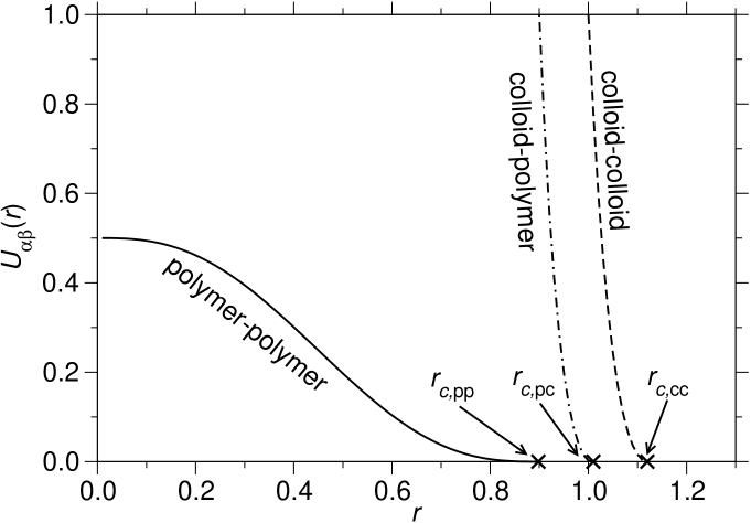
Note that the expansion in the square bracket of Eq. (4) is essentially a polynomial fit to a cosine function, which is shifted by unity and the angle of which varies from to when increases from zero to . However, while the cosine function is smoothly differentiable only once at and , Eq. (4) is twofold differentiable. Of course, . Note that the choice (5) differs from the original AO model only by replacing the original hard core interactions and by smooth interactions, Eqs. (1)-(3), while polymers are still strictly non-interacting. For the choice (6), which is the choice used for the MD work, the energy varies from to zero, Fig. 1. With these choices of potentials the application of MD is straightforward and efficient, but also the application of grand-canonical Monte Carlo methods is still well feasible.
However, as in our earlier study of static and dynamic critical phenomena of a symmetrical binary Lennard-Jones mixture Das et al. (2003, 2004, 2006a, 2006b) it is advantageous to apply Monte Carlo methods (in the fully grand-canonical -ensemble, with , being the chemical potentials of colloids and polymers, respectively, in the present case) to determine the static phase diagram of the colloid-polymer mixture. In particular, determining the critical densities of colloids and polymers (where densities are defined in terms of the particle numbers of colloids and polymers in the standard way , , being the volume of the simulation box) is a nontrivial matter. In the context of MD simulation, starting systems at states which fall within the two-phase coexistence region and beginning with an initially homogeneous distribution of both types of particles lead to a phase separation into a “liquid-like” phase (with densities , ) and a “vapor-like” phase (with densities , ). Of course, a priori all the values of densities along the coexistence curve in the -plane are unknown and simulating the dynamics of spinodal decomposition is a complicated and notoriously slow process Binder and Fratzl (2001); Yelash et al. (2008). Moreover, when approaching the critical point (from the one-phase region or along the coexistence curve) simulations in the canonical ensemble suffer severely from critical slowing down Hohenberg and Halperin (1977) as discussed in Das et al. (2006a, b).
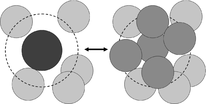
Thus, it is very desirable to study the phase behavior by Monte Carlo simulations in the grand-canonical ensemble, which turned out to be very useful for both the symmetrical binary Lennard-Jones mixture Das et al. (2006a) and the standard AO model Vink and Horbach (2004a, b). a number of well-equilibrated system configurations as initial states for strictly microcanonical MD runs Das et al. (2003, 2004, 2006a, 2006b), one realizes averages corresponding to a well-defined temperature without the need to augment the MD code by a thermostat Allen and Tildesley (1987); Rapaport (1995). However, already for the standard AO model straightforward particle insertion Monte Carlo moves, which are necessary to realize the grand-canonical ensemble, are almost always rejected due to the large density of polymers in the system Vink and Horbach (2004a, b). For the standard AO model Vink and Horbach Vink and Horbach (2004a, b) could cope with this difficulty by implementing a cluster move. A similar cluster move is used here (Fig. 2). To maximize the efficiency of this algorithm, always all polymer particles are removed in the depletion zone when a colloid is inserted. The radius of the depletion zone was . At most polymers would be inserted or removed in one attempted cluster move.
When this algorithm is applied to soft potentials, slight modifications of the implementation are required: Colloid deletion attempts must always be rejected if any center of polymer particles is located in the depletion zone. Otherwise, colloid insertion and deletion moves are no longer symmetric and detailed balance is violated. Note that this problem does not occur in the original AO model because polymer particles can never “overlap” with colloid particles. Note that the algorithm is still ergodic, because “overlaps” with the colloidal particles can be obtained by removing adjacent colloids and filling the void with polymer particles. Nevertheless it is still recommendable to mix cluster moves with local moves.
We wish to compare our results with the original AO model (with hard core interactions), where it is standard practice to use the packing fractions as variables,
| (7) |
where and are the volumes occupied by a colloid and polymer, respectively, with and , and being the diameters of colloids and polymers. For this comparison it is hence useful to define an effective diameter of colloids and polymers of our model using the approach of Barker and Henderson Barker and Henderson (1967)
| (8) |
Using Eqs. (1), (2) in Eq. (8) yields
| (9) |
and . We also use and consequently derive the following formulas to convert our densities into packing fractions
| (10) |
Hence, the polymer reservoir packing fraction Lekkerkerker et al. (1992); Vink and Horbach (2004a, b) is given by in terms of the chemical potential of the polymers. Of course, for interacting polymers the notion of loses its original meaning, but we continue to use as defined here for the sake of comparability with the standard AO model.
The technical aspects of grand-canonical Monte-Carlo simulations of phase equilibria and critical phenomena in colloid-polymer mixtures have been described in detail in the literature Vink and Horbach (2004a, b); Vink et al. (2005a); Binder et al. (2008). Therefore, we recall only very briefly the most salient features. Choosing and hence as a parameter, the chemical potential of the colloids is varied and the distribution of the colloid volume fraction is sampled, applying the cluster algorithm mentioned above. For sufficiently less than the critical volume (note that plays the role of inverse temperature, when the phase diagram of the colloid-polymer mixture is compared to the vapor-liquid phase separation of a molecular system) has a single peak at and the task is straightforward. For and near , however, is a doubly-peaked function where (apart from finite size effects Vink and Horbach (2004a, b); Vink et al. (2005a); Binder (1981); Binder and Landau (1984); Binder (1997)) the positions of the two peaks correspond to the volume fractions of the vapor-like phases at the coexistence curve, and . Since the distribution develops a very deep minimum in between these peaks Binder (1997, 1982), sampling is, however, not completely straightforward. An efficient way to overcome this difficulty is provided by successive umbrella sampling Virnau and Müller (2004), which was applied in this work. The chemical potential at vapor-liquid coexistence is then given by the equal weight rule Borgs and Kotecky (1990), i.e. the areas underneath the peaks corresponding to the vapor-like phase and the liquid-like phase have to be equal. The order parameter of the phase transition can then be identified as
| (11) |
with being the average of including both peaks at . A convenient tool to find the critical value is based on the analysis of moment ratios , defined as Binder (1981, 1997)
| (12) |
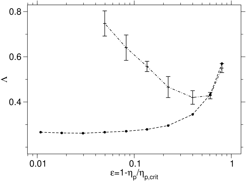
while following a path along for different linear dimensions of the cubic simulation box. The critical value is determined found from the intersection of these curves. Figure 3 gives an example for the present model. Note that the procedure described above is also operationally well defined for a range of values , since due to finite size effects, the distribution is double-peaked over some range in the one-phase region as well Binder (1981, 1997). It can be recognized from Fig. 3 that a rather well-defined intersection point occurs for . However, this intersection does not occur at the theoretical value Luijten et al. (2002) but at a somewhat lower value . This discrepancy is due to various corrections to finite size scaling, in particular the so-called field mixing effects Wilding (1995, 1997). In the case of the standard AO model, a very similar discrepancy occurs as well Vink and Horbach (2004a, b). Since in the latter model no potential energy is present, the field mixing does not involve a coupling between energy density and density as for ordinary fluids Wilding (1995, 1997) but rather a coupling between colloid density and polymer density. So the order parameter (in the sense of a scaling field Wilding (1995, 1997)) is in a strict sense not given by alone (as assumed in Eq. (11)). Instead, a suitable linear combination of and needs to be constructed. However, we have not done this in the context of finding the critical point since there is ample evidence in various systems Virnau et al. (2004); Pérez-Pellitero et al. (2006); Mognetti et al. (2008) that the simple cumulant intersection method as illustrated in Fig. 3 does yield the critical point with a relative accuracy of a few parts in a thousand, which suffices for the present purposes.
III Static properties of the soft version of the AO model
As discussed in Sec. II, the first step of the Monte Carlo study consists of the estimation of the coexistence curve and the critical point. For the two models defined in Eqs. (5),(6) we found for
| (13) |
and for
| (14) |
Since the accuracy of these numbers is about , we conclude that model (i), the “soft AO model”, is within our errors not distinguishable from the original AO model with hard core interactions for which the analogous results are Vink and Horbach (2004a, b)
| (15) |
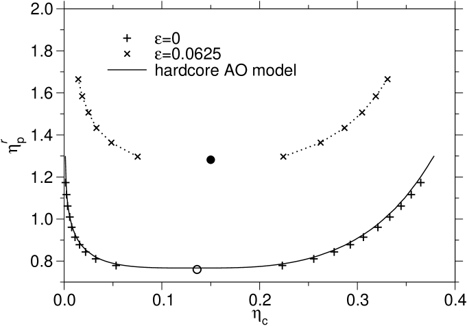
This coincidence between the soft AO model and its hard core version is also seen in the coexistence curve, which is compared in reservoir representation in Fig. 4. The coexistence curve of the model with interacting polymers is substantially different, of course, as expected from Eq. (14).
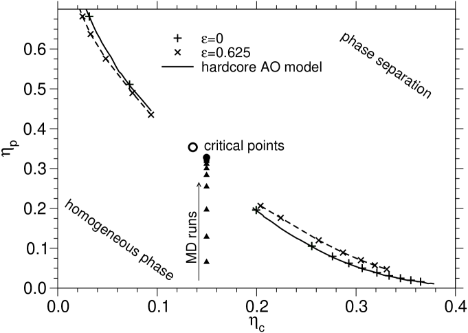
However, when we study phase coexistence as a function of all experimentally accessible variables , differences between the three models are rather minor (Fig. 5). It appears that near criticality the main effect of “switching on” the polymer-polymer interaction is to shift the critical point along the coexistence curve of the AO model to the higher value of (and correspondingly lower value of mentioned in Eq. (14). Further away from the critical point the coexistence curve of the interacting polymer model predicts somewhat lower polymer packing fractions along the “vapor branch” and somewhat higher polymer packing fractions along the “liquid branch”. The result that the critical packing fraction of polymers is about twice that of the colloids is similar to what was observed in a recent experiment Hennequin et al. (2008). Note however, that in these experiments a size ratio of polymers to colloids of (rather than ) was employed which affects ( was found in Hennequin et al. (2008)).
In Fig. 5 we have also indicated the state points at which micro-canonical MD runs took place. We have fixed the number of colloids in a volume (of size ) such that (which corresponds to ). Then the number of polymers was varied from zero up to . The MD runs were carried out with the Velocity Verlet algorithm Allen and Tildesley (1987); Rapaport (1995) and a time step . The masses of colloids and polymers are equal and units of time are chosen such that . In the production runs used for the computation of time-displaced correlation functions no thermostat was applied, so a microcanonical ensemble respecting all conservation laws applies. Starting configurations were generated as follows: First, a random configuration was generated in a box of linear dimension and periodic boundary conditions. The system was equilibrated at for million time steps with a simple velocity rescaling according to the Maxwell-Boltzmann distribution. Then, the system is enlarged from to by replicating it three times in all spatial directions. Now periodic boundary condition for only are applied. Equilibration is continued for 2 million time steps, again with a Maxwell-Boltzmann thermostat. During this equilibration, the original periodicity with is quickly lost. The production runs for static averages are done without applying any thermostat. First, 5 million time steps are performed during which (at eight different times) statistically independent configurations are stored. These serve as starting configurations for eight independent simulation runs, each with 5 million steps, for the computation of static averages. During each run, 500 configurations are analyzed in regular intervals. Thus, 4000 statistically independent configurations are averaged over for the computation of the structure factor.
From now on, we denote colloids as A-particles and polymers as B-particles. For all simulated state points the partial structure factors were computed,
| (16) |
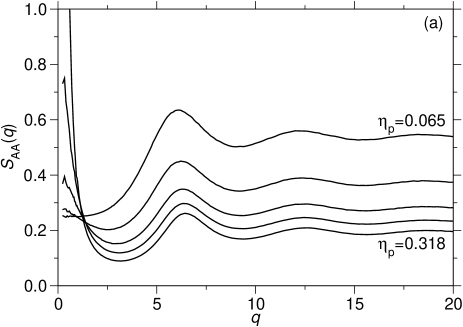
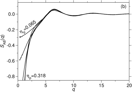
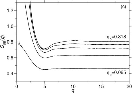
with . These results, presented in Figs. 6(a)-(c), show that the partial structure factor for colloids (Fig. 6(a)) displays an oscillatory structure with a first peak near , which is typical for the packing of hard particles in a moderately dense liquid. The partial structure factor due to polymers (Fig. 6(c)) exhibits much less structure in the range of large as expected, since for the potential, Eq. (4), the polymers can still overlap rather easily. All these partial structure factors show a strong enhancement at small , reflecting the critical scattering due to the unmixing tendency between colloids and polymers when the critical point is approached. Note that the partial structure factor due to interference of the scattering from colloids and polymers (Fig. 6(b)) also shows oscillations at large , as does the scattering from colloids alone (Fig. 6(a)).
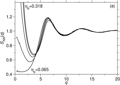
From the partial structure factors it is useful to construct combinations that single out number-density fluctuations and concentration fluctuations , defined via Bhatia and Thornton (1970) (, )
| (17) | ||||
| (18) |
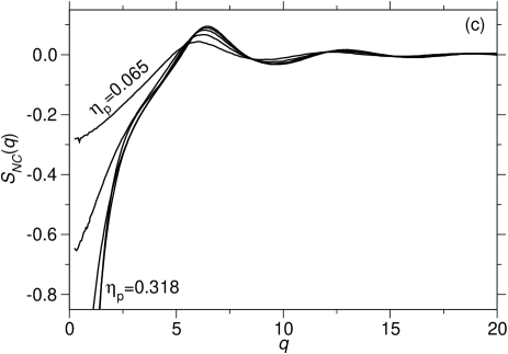
In addition, it is of interest to consider a structure factor relating to the coherent interference of number density and concentration fluctuations Bhatia and Thornton (1970),
| (19) |
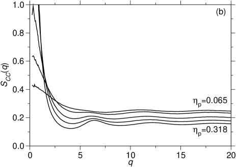
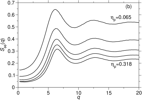
Figure 7 shows that all three structure factors show a strong increase at small , reflecting the critical scattering as the critical point is approached. Additionally, at large they display oscillations. The behavior seen in Fig. 7 differs very much from the behavior found for the unmixing of the symmetric binary Lennard-Jones mixture Das et al. (2003, 2004, 2006a, 2006b). In the latter case was not sensitive to the critical fluctuations at all, which showed up in only. Likewise, was insensitive to the way how the particles are “packed” in the liquid, i.e. there was no structure at large . In addition, almost no interference between the scattering from concentration and density fluctuations could be seen. Hence, was very small, while in the present model and are of the same order of magnitude. These observations clearly show that neither the total density in the system, nor the relative concentration of one species is a “good” order parameter of the phase separation that occurs. (Likewise, Fig. 6 shows that neither the colloid density alone nor the polymer density alone are “good” order parameters since both densities reflect the critical scaling in a similar way.) Of course, from the phase diagram (Fig. 5) such a problem is expected since the shape of the coexistence curve shows that the order parameter is a nontrivial linear combination of both particle numbers .
In order to deal with this problem, we introduce a symmetrical matrix formed from the structure factors , and
| (20) |
and diagonalize this matrix to obtain its diagonal form
| (21) |
with
| (22) |
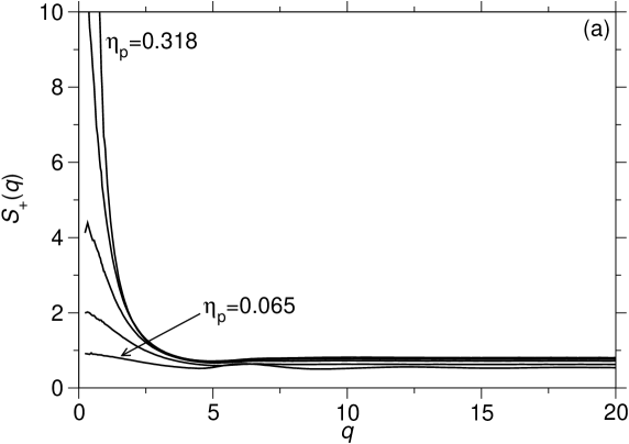
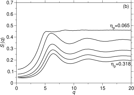
Figure 8 shows a plot of and versus . This plot shows that this procedure indeed resulted in a decoupling of the order parameter fluctuations (which show a critical enhancement as ), as being measured by , and the noncritical “particle packing” fluctuations, measured by , which show the characteristic oscillatory structure of a noncritical fluid. In the case of the symmetrical LJ mixture the transformation from the number density fluctuations of A and B particles to the structure factors measuring the fluctuations of the total density of particles and of their relative concentrations is unambiguous. In the case of the colloid-polymer mixture it is none of these variables which plays the role of an order parameter, but a different linear combination of both local densities of A and B particles, related to the eigenvector corresponding to . We can give this fact a plausible interpretation by constructing two linear combinations of the operators , , defined via , as follows
| (23) | ||||
| (24) |
The coefficients are defined such that at the critical point the densities lie tangential to the coexistence curves. Coefficients are chosen such that the densities vary in a perpendicular direction to this slope. When we construct the structure factors (Fig. 9)
| (25) |
one recognizes that is very similar to and very similar to . The structure factors defined in this manner are not strictly identical to . With increasing distance from criticality the relative weights , of the components of the “order parameter components” change.
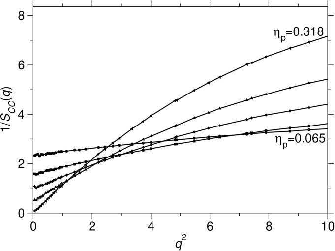
For all those structure factors that show a critical increase can be described by the well-known Ornstein-Zernike behavior. This is illustrated in Fig. 10, as an example, for the concentration, fitting versus at small enough () to the relation Hansen and McDonald (1986); Das et al. (2006b)
| (26) |
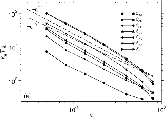
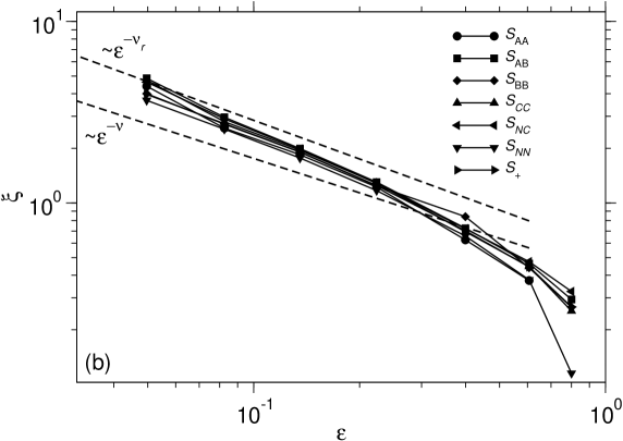
Here, is the “susceptibility” describing the magnitude of concentration fluctuations and the correlation length. The various susceptibilities relating to the various structure factors defined above and the associated correlation ranges are shown in Fig. 11. It is gratifying to note that indeed the “susceptibility” related to is the largest susceptibility that can be found, while the estimates for the correlation lengths are all equal (within statistical errors). Due to the coupling between variables, there is only a single correlation length in the problem.
In Fig. 11 we have included two theoretical predictions in the log-log plot for the critical exponents, one is a slope corresponding to the standard Ising exponents (that are observed in the grand-canonical ensemble, where only intensive thermodynamic variables are held constant). The other slope shows the exponents if “Fisher renormalization” occurs. To remind the reader of this phenomenon we note that the response function that is observed via Monte Carlo from the fluctuation relation
| (27) |
differs from since fluctuations differ in different ensembles of statistical mechanics. While was estimated from Eq. (26) which refers to the ensemble where , Eq. (27) refers to the ensemble where . Since Fisher (1968)
| (28) |
where is the specific heat exponent and are constants. Very close to the critical point we have a singular relation between and , namely
| (29) |
Therefore the power laws in the grand-canonical ensemble Zinn-Justin (2001); Binder and Luijten (2001)
| (30) |
translate into power laws with “Fisher renormalized” Fisher (1968) exponents in the microcanonical ensembles where are constant
| (31) |
However, since the regular third term on the right hand side of Eq. (28) is comparable to the (singular) second term that was only used in Eq. (29), except if one works extremely close to , it is difficult to ascertain whether or not the simulation data shows any signature of Fisher renormalization. High precision simulations for very much larger systems would be required to clearly resolve this issue. This task, however, is not possible with presently available computer resources.
It is also useful to recall that susceptibilities observed in the grandcanonical ensemble differ from those extracted from structure factors in the canonical ensemble. To interpret this difference, we start from the standard relation for the grandcanonical partition function
| (32) |
from which one straightforwardly derives the following fluctuation relations ():
| (33) | ||||||
| (34) |
and
| (35) |
It is this mixed susceptibility describing the correlations between the fluctuations of colloid and polymer number which enters the difference between the susceptibilities in the canonical and grandcanonical ensemble. A simple calculation yields
| (36) |
Similarly,
| (37) |
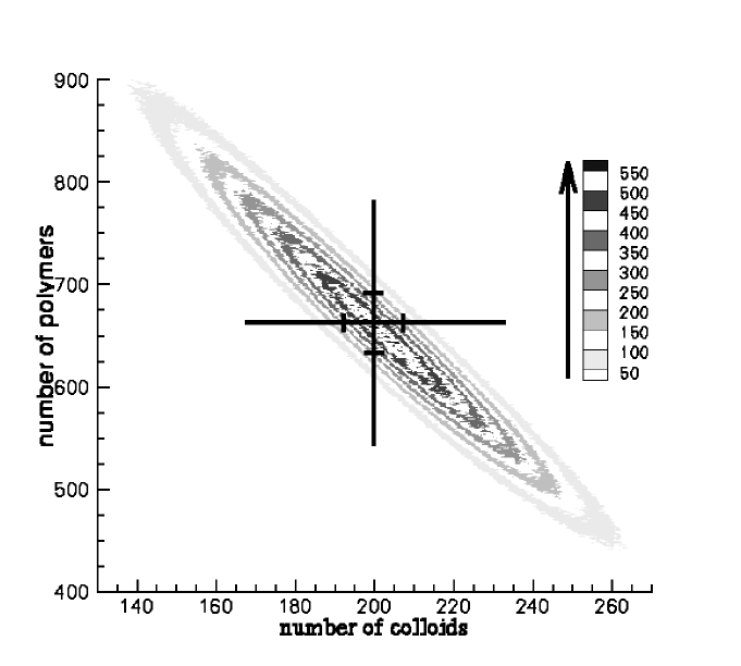
In fully grand-canonical simulations, as we have carried out in the present work, it is possible to extract all susceptibilities of interest from a study of the joint distribution function . In the one phase region and for large enough linear dimensions this function is a bivariate Gaussian in the variables , , see Fig. 12 for an explicit example. Then the fluctuations and can be extracted from the half-widths of these distributions along the abscissa direction () and ordinate direction , respectively. For the grand-canonical simulations described in Fig.12, for example, we obtain and 0.05 for the second equation in (36) thus confirming our calculations. Figure 12 illustrates again that none of these susceptibilities should be regarded as the order parameter susceptibility : rather the latter is the half-width along the main axis of the ellipsoidal contours in Fig. 12.
IV Dynamics of colloid-polymer mixtures
From the MD runs it is straightforward to obtain the incoherent intermediate scattering functions defined as ()
| (38) |
as well as time-displaced mean square displacements of the particles
| (39) |
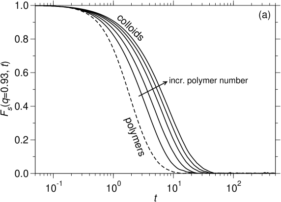
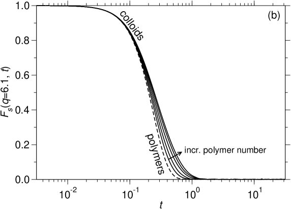
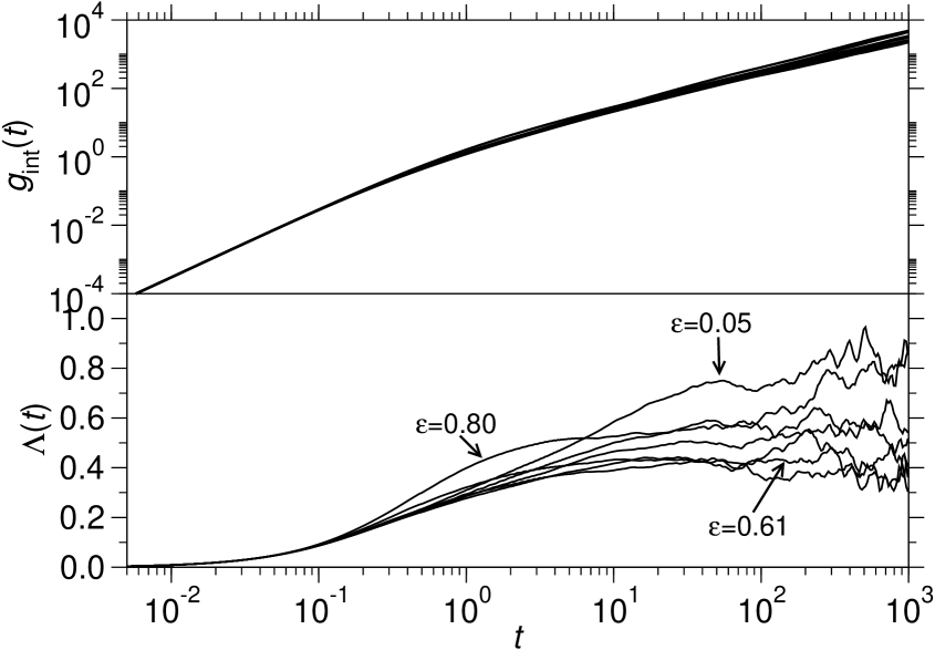
In the MD framework the average stands for an average over the origins of time, (we have used 8 statistically independent runs and two time origins per run, thus we have averaged over time origins). Figure 13 shows typical data for both small and large . For the colloids there is some uniform slowing down of at small as increases, while for large (near the first peak of ) the decay occurs in two parts: the first part (for ) is basically independent of , while for the curves distinctly splay out. In contrast, the analogous function for the polymers seems to be practically independent of , irrespective of .
A similar asymmetry between the dynamics of colloids and polymers is also seen in the mean square displacements. Since we expect for large times the Einstein relation to hold,
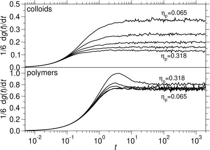
| (40) |
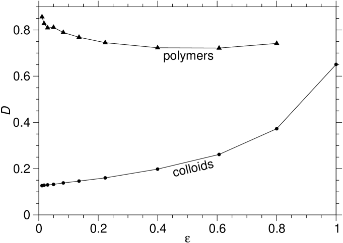
we analyze the derivative (Fig. 14). From the plateau of this quantity at large times, one can see that approaches its asymptotic behavior for colloids monotonically while for polymers there is an overshoot for intermediate times, . In the regime of this transient maximum the data depends rather distinctly on . In the asymptotic regime () the dependence is much weaker. The time range where this overshoot occurs is related to the crossover from ballistic to diffusive motion. For both colloids and polymers show a ballistic behavior, , as expected Allen and Tildesley (1987); Rapaport (1995). Of course, no such behavior is expected for real colloid-polymer mixtures, where the solvent molecules (no explicit solvent is included in our simulations, of course) damp out the “free flight” motion present in our model. Instead, one would find another diffusive motion controlled by the solvent viscosity. Figure 15 shows that the resulting selfdiffusion constants are of similar magnitude for small (very far from ) but differ by almost an order of magnitude when is approached.
Finally, we consider the interdiffusion between colloids and polymers. Defining the center of mass coordinate of the particles of species as , we note that interdiffusion is related to the following mean square displacement () Hansen and McDonald (1986); Horbach et al. (2007)
| (41) |
Note that is computed via the integral with the center of mass velocity of component A and the velocity of particle at time . In this manner one obtains the difference in an origin independent representation Allen and Tildesley (1987); Horbach et al. (2007). The Onsager coefficient relating to interdiffusion can be expressed as
| (42) |
The interdiffusion constant , which describes how concentration fluctuations in the binary (A,B)-system relax, is then given as the ratio of the Onsager coefficient and the “concentration susceptibility” , where
| (43) |
Note that theory Kawasaki (1970a, b); Luettmer-Strathmann et al. (1995); Luettmer-Strathmann and Sengers (1996); Sengers (1985) predicts that contains two terms, a background term which is nonsingular and stays finite at the critical point and a critical term which diverges at the critical point,
| (44) |
with an exponent Siggia et al. (1976); Ferrell and Bhattacharjee (1985); Hao et al. (2005). In fact, a recent MD study of the critical dynamics of the symmetric binary Lennard-Jones mixture Das et al. (2006a, b) yielded results compatible with this theoretical prediction, Eq. (44). This allows to estimate the noncritical background term at the critical point, too. Thus, it is also of great interest to study the behavior of when we approach the critical point of our model (Fig. 17). Here, we have also included the simple prediction of the Darken equation Darken (1049),
| (45) |
While very far from criticality , Eq. (45) indeed describes the simulation results accurately, it underestimates strongly for closer to , and clearly Eq. (45) violates Eq. (44). Thus, Darken’s equation Darken (1049) fails near the critical point of a fluid binary mixture as it was already noted for the binary Lennard-Jones mixture Binder et al. (2007).
Thus, we see from Fig. 17 that for our asymmetric mixture we also find evidence for a singular behavior of the Onsager coefficient for interdiffusion. However, the statistical accuracy of the data for does not warrant an attempt to estimate the dynamic critical exponent (in particular since this is rather difficult here to estimate ). The statistical effort invested is just enough to allow an approach of criticality up to about , but not closer. In order to allow meaningful estimates of , , and , the time of a simulation run must be at least about an order of magnitude longer than the time needed for a concentration fluctuation to relax via interdiffusion. This time is
| (46) |
From Figs. 11(a),(b) and 17 we see for that , , and , yielding . Since , the run at is just long enough, but data closer to criticality cannot be used. The estimate Eq. (46) is compatible with a direct examination of , Fig. 16, where we see that far away from criticality a plateau is only reached when .
Another condition for the validity of our result is that the initial periodicity width has fully relaxed. This equilibration time of our system is estimated in analogy to Eq. (46) as for . The actual equilibration time of MD time units indeed exceeds this estimate by a factor of about two. So our data should be valid but it is hardly possible to approach criticality closer. Finally, since no attempt of a finite size scaling analysis of the dynamical properties is made here (unlike Das et al. (2006a, b)), we have to require that at the states of interest. Though this condition holds for , it would fail if we approach the critical point much closer. From this discussion we see that a substantially larger computational effort would be required for a more detailed analysis of the dynamic critical behavior of this model.
V Summary
In this paper, a model of colloid-polymer mixtures has been introduced and studied, which uses continuous potentials between all types of particles. Nevertheless, it still resembles closely the Asakura-Oosawa (AO) model, as far as static properties are concerned. The chosen potentials (Eqs. (1)-(6)) are clearly somewhat arbitrary: the choice of these potentials was motivated by the desire that the model should be suitable for grand-canonical Monte Carlo methods to accurately establish the phase diagram (Figs. 4, 5). In addition, it should allow for a convenient and physically meaningful application of Molecular Dynamics techniques. In this way, both static and dynamic behavior of such a phase-separating strongly asymmetric binary mixture, where phase separation is mainly driven by entropic depletion effects, has become accessible to a computer simulation study.
Previous simulation studies have mostly been concerned with the phase diagram of the AO model and related models as well as the interfacial tension between coexisting polymer-rich and colloid-rich phases. The present work contains a detailed analysis of the various static structure factors , and that one can define in such a binary (AB) mixture, and suitable linear combinations of them that single out the order parameter of the unmixing transition. Unlike other models of (almost incompressible) binary mixtures, in the present system the relative concentration of one species is not the proper order parameter. Instead the order parameter is a nontrivial combination of polymer density and colloid density fluctuations, which can be found from diagonalizing the structure factor matrix. From this analysis, we can study the onset of the critical divergence of both the order parameter “susceptibility” and correlation length. Roughly, these results are compatible with the expected Ising-like criticality. Fine details such as whether Fisher renormalization of critical exponents occur can, unfortunately, not be clarified, since our data are restricted to relative distances from the critical point exceeding . Of course, for reliable statements on critical exponents data somewhat closer to the critical point are indispensable, but at present not yet available.
A central part of our study concerns the analysis of time-dependent quantities, intermediate incoherent structure factors and mean square displacements, and their analysis. While the self-diffusion constant of the colloids is decreasing monotonously with increasing polymer density, surprisingly the self-diffusion constant of the polymers shows a slight increase. Thus, there is a pronounced dynamic asymmetry of our model. The Onsager coefficient relating to interdiffusion is also obtained, and qualitative evidence for a critical divergence is found, thus invalidating the simple Darken equation for this system. However, the present data do not yet allow an accurate estimation of dynamic critical exponents for the colloid-polymer mixture. More efficient algorithms (or significantly faster computers) will be needed for a more definite study of critical behavior in our model system. Nevertheless, we hope that our study will motivate related experimental work on the dynamics of colloid-polymer mixtures, to which some of our findings could be compared directly.
Acknowledgments
This work received financial support from the Deutsche Forschungsgemeinschaft, TR6/A5. Computing time on the JUMP at the NIC Jülich is gratefully acknowledged.


References
- Poon and Pusey (1995) W. C. Poon and P. N. Pusey, in Observation, Prediction and Simulation of Phase Transitions in Complex Fluids, edited by M. Baus, L. F. Rull, and J. P. Ryckaert (Kluwer Acad. Publ., Dordrecht, 1995), pp. 3–51.
- Lekkerkerker et al. (1995) H. N. W. Lekkerkerker, P. Buining, J. Britenhuis, C. G. Vroege, and A. Stroebants, in Observation, Prediction and Simulation of Phase Transitions in Complex Fluids, edited by M. Baus, L. F. Rull, and J. P. Ryckaert (Kluwer Acad. Publ., Dordrecht, 1995), pp. 53–112.
- Arora and Tata (1998) A. K. Arora and B. V. R. Tata, Adv. Colloid Interface Sci. 78, 49 (1998).
- Löwen (2001) H. Löwen, J. Phys.: Condensed Matter 13, R415 (2001).
- Löwen and Likos (2004) H. Löwen and C. N. Likos, eds., Special Issue: Colloidal Dispersions in External Fields, J. Phys.: Condensed Matter 16, no. 38 (2004).
- Blaaderen (1997) A. Blaaderen, Progr. Colloid Polym. Sci. 104, 59 (1997).
- Asakura and Oosawa (1954) S. Asakura and F. Oosawa, J. Chem. Phys. 22, 1255 (1954).
- Asakura and Oosawa (1958) S. Asakura and F. Oosawa, J. Polym. Sci. 33, 183 (1958).
- Vrij (1976) A. Vrij, Pure Appl. Chem. 48, 471 (1976).
- Gast et al. (1983) A. P. Gast, C. K. Hall, and W. B. Russel, J. Colloid Interface Sci. 96, 251 (1983).
- Lekkerkerker et al. (1992) H. N. W. Lekkerkerker, W. C. Poon, P. Pusey, A. Stroebants, and P. Warren, Europhys. Lett. 20, 599 (1992).
- Ilett et al. (1995) S. M. Ilett, A. Orrock, W. C. K. Poon, and P. N. Pusey, Phys. Rev. E 51, 1344 (1995).
- Aarts et al. (2004) D. G. A. L. Aarts, M. Schmidt, and H. N. W. Lekkerkerker, Science 304, 847 (2004).
- Wijting et al. (2003) W. K. Wijting, N. A. M. Besseling, and M. A. C. Stuart, Phys. Rev. Lett. 90, 196101 (2003).
- Aarts (2005) D. G. A. L. Aarts, J. Phys. Chem. B 109, 7407 (2005).
- Hennequin et al. (2008) Y. Hennequin, D. G. A. L. Aarts, J. O. Indekeu, H. N. W. Lekkerkerker, and D. Bonn, Phys. Rev. Lett. 100, 178305 (2008).
- Royall et al. (2007) C. P. Royall, D. G. A. L. Aarts, and H. Tanaka, Nature Physics 3, 636 (2007).
- Derks et al. (2006) D. Derks, D. G. A. L. Aarts, D. Bonn, H. N. W. Lekkerkerker, and A. Imhof, Phys. Rev. Lett. 97, 038301 (2006).
- Aarts and Lekkerkerker (2004) D. G. A. L. Aarts and H. N. W. Lekkerkerker, J. Phys.: Condensed Matter 16, S4231 (2004).
- Vink and Horbach (2004a) R. L. C. Vink and J. Horbach, J. Chem. Phys. 121, 3253 (2004a).
- Vink and Horbach (2004b) R. L. C. Vink and J. Horbach, J. Chem. Phys. 16, S3807 (2004b).
- Vink et al. (2005a) R. L. C. Vink, J. Horbach, and K. Binder, Phys. Rev. E 71, 011401 (2005a).
- Vink et al. (2005b) R. L. C. Vink, J. Horbach, and K. Binder, J. Chem. Phys. 122, 134905 (2005b).
- De Virgiliis et al. (2007) A. De Virgiliis, R. L. C. Vink, J. Horbach, and K. Binder, Europhys. Lett. 77, 60002 (2007), and preprint.
- Binder et al. (2008) K. Binder, J. Horbach, R. Vink, and A. De Virgiliis, Soft Matter 4, 1555 (2008).
- Schmidt et al. (2003) M. Schmidt, A. Fortini, and M. Dijkstra, J. Phys.: Condensed Matter 15, S3411 (2003).
- Schmidt et al. (2004) M. Schmidt, A. Fortini, and M. Dijkstra, J. Phys.: Condensed Matter 16, S4159 (2004).
- Schmidt et al. (2006) M. Schmidt, A. Fortini, and M. Dijkstra, Phys. Rev. E 73, 051502 (2006).
- Vink et al. (2006a) R. L. C. Vink, K. Binder, and J. Horbach, Phys. Rev. E 73, 056118 (2006a).
- Vink et al. (2006b) R. L. C. Vink, A. De Virgilis, J. Horbach, and K. Binder, Phys. Rev. E 74, 069903 (2006b).
- Dijkstra and van Roij (2002) M. Dijkstra and R. van Roij, Phys. Rev. Lett. 89, 128302 (2002).
- Brader et al. (2002) J. M. Brader, R. Evans, M. Schmidt, and H. Löwen, J. Phys: Condensed Matter 14, L1 (2002).
- Fortini et al. (2005) A. Fortini, M. Dijkstra, M. Schmidt, and P. P. F. Wessels, Phys. Rev. E 71, 051403 (2005).
- Dijkstra et al. (2006) M. Dijkstra, R. van Roij, R. Roth, and A. Fortini, Phys. Rev. E 73, 041404 (2006).
- Brader and Evans (2000) J. M. Brader and R. Evans, Europhys. Lett. 49, 678 (2000).
- Meijer and Frenkel (1994) E. J. Meijer and D. Frenkel, J. Chem. Phys. 100, 6873 (1994).
- Bolhuis et al. (2002) P. G. Bolhuis, A. A. Louis, and J.-P. Hansen, Phys. Rev. Lett. 89, 128302 (2002).
- Bolhuis et al. (2001) P. G. Bolhuis, A. A. Louis, J.-P. Hansen, and E. J. Meyer, J. Chem. Phys. 114, 4296 (2001).
- Chou et al. (2006) C. Y. Chou, T. T. M. Vo, A. Z. Panagiotopoulos, and M. Robert, Physica A 369, 275 (2006).
- Bolhuis and Louis (2002) P. G. Bolhuis and A. A. Louis, Macromolecules 35, 1860 (2002).
- Louis (2002) A. A. Louis, J. Phys.: Condensed Matter 14, 9187 (2002).
- R.Rotenberg et al. (2004) R.Rotenberg, J. Dzubiella, A. A. Louis, and J.-P. Hansen, Mol. Phys. 102, 1 (2004).
- Landau and Binder (2005) D. P. Landau and K. Binder, A Guide to Monte Carlo Simulation in Statistical Physics (Cambridge University Press, Cambridge, 2005), 2nd ed.
- Allen and Tildesley (1987) M. P. Allen and D. J. Tildesley, Computer Simulation of Liquids (Clarendon Press, Oxford, 1987).
- Rapaport (1995) D. C. Rapaport, The Art of Molecular Dynamics Simulation (Cambridge University Press, Cambridge, 1995).
- de Gennes (1979) P. G. de Gennes, Scaling Concepts in Polymer Physics (Cornell University Press, Ithaca, 1979).
- Hansen and McDonald (1986) J. P. Hansen and I. R. McDonald, Theory of simple liquids (Academic Press, San Diego, 1986).
- Das et al. (2003) S. K. Das, J. Horbach, and K. Binder, J. Chem. Phys. 119, 1547 (2003).
- Das et al. (2004) S. K. Das, J. Horbach, and K. Binder, Phase Transitions 77, 823 (2004).
- Das et al. (2006a) S. K. Das, M. E. Fisher, J. V. Sengers, J. Horbach, and K. Binder, Phys. Rev. Lett. 97, 025702 (2006a).
- Das et al. (2006b) S. K. Das, J. Horbach, K. Binder, M. E. Fisher, and J. V. Sengers, J. Chem. Phys. 125, 024506 (2006b).
- Binder and Fratzl (2001) K. Binder and P. Fratzl, in Phase Transformations in Materials, edited by G. Kostorz (VCH-Wiley, Weinheim, 2001), p. 409.
- Yelash et al. (2008) L. Yelash, P. Virnau, W. Paul, M. Müller, and K. Binder, Phys. Rev. E 78, 031801 (2008).
- Hohenberg and Halperin (1977) P. C. Hohenberg and B. I. Halperin, Rev. Mod. Phys. 49, 435 (1977).
- Barker and Henderson (1967) J. A. Barker and J. Henderson, J. Chem. Phys. 47, 4714 (1967).
- Binder (1981) K. Binder, Z. Phys. B: Condensed Matter 43, 119 (1981).
- Binder and Landau (1984) K. Binder and D. P. Landau, Phys. Rev. B 30, 1477 (1984).
- Binder (1997) K. Binder, Rep. Progr. Phys. 60, 487 (1997).
- Binder (1982) K. Binder, Phys. Rev. A 25, 1699 (1982).
- Virnau and Müller (2004) P. Virnau and M. Müller, J. Chem. Phys. 120, 10925 (2004).
- Borgs and Kotecky (1990) C. Borgs and R. Kotecky, J. Stat. Phys. 61, 79 (1990).
- Luijten et al. (2002) E. Luijten, M. E. Fisher, and A. Z. Panagiotopoulos, Phys. Rev. Lett. 88, 185701 (2002).
- Wilding (1995) N. B. Wilding, Phys. Rev. E 52, 602 (1995).
- Wilding (1997) N. B. Wilding, J. Phys.: Condensed Matter 9, 585 (1997).
- Virnau et al. (2004) P. Virnau, M. Müller, L. G. MacDowell, and K. Binder, J. Chem. Phys. 121, 2169 (2004).
- Pérez-Pellitero et al. (2006) J. Pérez-Pellitero, P. Ungerer, G. Orkoulas, and A. D. Mackie, J. Chem. Phys. 125, 054515 (2006).
- Mognetti et al. (2008) B. M. Mognetti, M. Oettel, L. Yelash, P. Virnau, W. Paul, and K. Binder, Phys. Rev. E 77, 041506 (2008).
- Bhatia and Thornton (1970) A. B. Bhatia and D. E. Thornton, Phys. Rev. B 2, 3004 (1970).
- Fisher (1968) M. E. Fisher, Phys. Rev. 176, 257 (1968).
- Zinn-Justin (2001) J. Zinn-Justin, Phys. Rep. 344, 159 (2001).
- Binder and Luijten (2001) K. Binder and E. Luijten, Phys. Rep. 344, 179 (2001).
- Horbach et al. (2007) J. Horbach, S. K. Das, A. Griesche, M.-P. Macht, G. Frohberg, and A. Meyer, Phys. Rev. B 75, 174304 (2007).
- Kawasaki (1970a) K. Kawasaki, Ann. Phys. 61, 1 (1970a).
- Kawasaki (1970b) K. Kawasaki, Phys. Rev. A 1, 1750 (1970b).
- Luettmer-Strathmann et al. (1995) J. Luettmer-Strathmann, J. V. Sengers, and G. A. Olchowy, J. Chem. Phys. 103, 7482 (1995).
- Luettmer-Strathmann and Sengers (1996) J. Luettmer-Strathmann and J. V. Sengers, J. Chem. Phys 104, 3026 (1996).
- Sengers (1985) J. V. Sengers, Int. J. Thermophys. 6, 203 (1985).
- Siggia et al. (1976) E. D. Siggia, B. I. Halperin, and P. C. Hohenberg, Phys. Rev. B 13, 2110 (1976).
- Ferrell and Bhattacharjee (1985) R. A. Ferrell and J. K. Bhattacharjee, Phys. Rev. A 31, 1788 (1985).
- Hao et al. (2005) H. Hao, R. A. Ferrell, and J. K. Bhattacharjee, Phys. Rev. E 71, 021201 (2005).
- Darken (1049) L. S. Darken, Trans. AIME 180, 430 (1049).
- Binder et al. (2007) K. Binder, S. K. Das, M. E. Fisher, J. Horbach, and J. V. Sengers, in Diffusion Fundamentals II, edited by S. Brandani, C. Chmelik, J. Kärger, and R. Volpe (Leipziger Universitätsverlag, 2007), p. 120.