Robust chaos with variable Lyapunov exponent in smooth one-dimensional maps

Abstract

We present several new easy ways of generating smooth one-dimensional maps displaying robust chaos, i.e., chaos for whole intervals of the parameter. Unlike what happens with previous methods, the Lyapunov exponent of the maps constructed here varies widely with the parameter. We show that the condition of negative Schwarzian derivative, which was used in previous works, is not a necessary condition for robust chaos. Finally we show that the maps constructed in previous works have always the Lyapunov exponent $\ln 2$ because they are conjugated to each other and to the tent map by means of smooth homeomorphisms. In the methods presented here, the maps have variable Lyapunov coefficients because they are conjugated through non-smooth homeomorphisms similar to Minkowski’s question mark function.

I Introduction

Many families of smooth maps display fragile chaos, which may be destroyed by arbitrarily small changes of the parameter. For instance, the discrete dynamical system generated by the logistic map, $x_{n+1}=\mu x_{n}\left(1-x_{n}\right)$, is chaotic for $\mu=4$, but the values of the parameter $\mu$ for which the attractor is periodic are dense in the interval $[0,4]$ Ott . In consequence, when such a family is used to describe a physical system, it may be impossible to decide on theoretical grounds whether the actual behavior of the system will be chaotic or periodic for some parameter value, which is necessarily known only approximately. Furthermore, some practical applications, such as encoding messages Hayes , require reliable chaotic behavior.

Piecewise smooth maps may show robust chaos and they have been used to describe a circuit with robust chaotic output Banerjee . Although for some time it was conjectured that one-dimensional maps should be piecewise smooth to display robust chaos Barreto ; Banerjee , Andrecut and Ali first found a smooth map Andrecut1 and later a method of generating smooth maps Andrecut2 whose evolution is chaotic for whole intervals of the parameter.

The purpose of this work is twofold: we want to explore other easy ways of generating robust chaos in one-dimensional smooth maps and to check whether the condition of negative Schwarzian derivative satisfied by the maps of Refs. Andrecut1 ; Andrecut2 is a necessary one. Unlike in previous methods, the Lyapunov exponent of the maps explored here takes rather different values depending on the value of the parameter. This property might be an advantage in some applications. We will see in Sect. IV that the reason of this dependence lies in the different ways in which maps generated by each method are conjugate to each other.

We will consider maps on a finite interval $[a,b]$, which for commodity will be reduced to $[0,1]$ by means of a linear transformation.

II Robust chaos with negative Schwarzian derivative

The Schwarzian derivative of the function $f$ is defined as

$$\operatorname{S}f(x)\equiv\frac{f^{\prime\prime\prime}(x)}{f^{\prime}(x)}-\frac{3}{2}\left(\frac{f^{\prime\prime}(x)}{f^{\prime}(x)}\right)^{2}.$$ (1)

Since Singer used it in the study of the bifurcations of maps of the interval Singer , a key assumption in many theorems on the dynamics of one-dimensional discrete dynamical systems is that the Schwarzian derivative of the map is negative along the whole interval.

In the following we will take advantage of the fact that the Schwarzian derivative is invariant under linear fractional transformations Jackson , i.e., that for constants $a$, $b$, $c$ and $d$ one has

$$\operatorname{S}\frac{af(x)+b}{cf(x)+d}=\operatorname{S}f(x).$$ (2)

Our starting point will be a map $f:[0,1]\to[0,1]$ of class $C^{3}$, which we assume to be ‘S-unimodal,’ i.e., which satisfies $f(0)=f(1)=0$, has a single critical point at $c\in(0,1)$, and negative Schwarzian derivative everywhere in $[0,1]$. Clearly $f$ increases from its null value at $x=0$ until it reaches its maximum at $x=c$, and then decreases until becoming 0 again at $x=1$. According to Singer’s theorem Singer ; Jackson , the discrete dynamical system $x_{n+1}=f(x_{n})$ has at most one stable periodic orbit, which when exists attracts the critical point $x=c$.

For any map $f$ with the properties above mentioned we will construct the following one-parameter family of maps:

$$f_{r}(x)\equiv\frac{(1+r)f(x)}{f(c)+rf(x)},\qquad(-1<r<\infty).$$ (3)

(Notice that $f_{r}$ does not change if one multiplies $f$ by any constant.)

By using (2) and

$$f_{r}^{\prime}(x)=\frac{(1+r)f(c)f^{\prime}(x)}{[f(c)+rf(x)]^{2}}$$ (4)

one can readily check that $f_{r}$ is also S-unimodal for all $r>-1$.

Now, for

$$r>r_{0}\equiv\frac{f(c)}{f^{\prime}(0)}-1,$$ (5)

the origin is a unstable fixed point, because then $f^{\prime}_{r}(0)>1$ and, furthermore, the dynamical system $x_{n+1}=f_{r}(x_{n})$ has no stable periodic orbit, because the critical point goes, in two steps, to the unstable origin: $f^{2}_{r}(c)=0$.

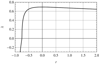
Figure 1: Lyapunov exponent of the map (3) for $f(x)=x(1-x)$.

To check that the dynamical system is chaotic for all $r>r_{0}$ on can compute numerically the Lyapunov exponent

$$\lambda=\lim_{N\to\infty}\sum_{n=1}^{N}{\ln\left|f_{r}^{\prime}\left(x_{n}\right)\right|}.$$ (6)

With the maps $f_{r}$ generated from the logistic map $f(x)=x(1-x)$ by means of (3), one gets the values displayed in Fig. 1. They are negative for $r<r_{0}=-3/4$, because then the origin is an attractor, and become positive at $r>r_{0}$ as the generic orbit wanders chaotically around the whole interval. In the maps generated in Refs. Andrecut1 ; Andrecut2 the Lyapunov coefficient was always $\ln 2$ or very close, according to the numerical simulations. In the maps presented above, the Lyapunov exponent varies with $r$ in a continuous way. If $f(x)=x(1-x)$ the maximum value of the Lyapunov exponent of $f_{r}(x)$ is $\lambda_{\mathrm{max}}=\ln 2$. This value is reached at $r=0$, which corresponds to the well known case $x_{n+1}=4x_{n}\left(1-x_{n}\right)$, which in turn is conjugate to the tent map defined as $f(x)=2x$ for $0\leq x\leq 1/2$ and $f(x)=2-2x$ for $1/2\leq x\leq 1$ Ott . Similar graphs, with $0<\lambda\leq\lambda_{\mathrm{max}}=\ln 2$, are obtained, for instance, for the asymmetric map $f(x)=x(1-x^{2})$ and for $f(x)=\sin\pi x$, although the bifurcation value $r_{0}$ and the location of the maximum are different.

Figure 2: Natural invariant density of the map (3) for $f(x)=x(1-x)$ and $r=0$ (dashed line) and $r=1$ (continuous line).

One can also compute numerically the natural invariant measure $d\mu=\rho_{r}(x)\,dx$ by using the Frobenius-Perron equation Ott satisfied by the natural invariant density $\rho_{r}(x)$:

$$\rho_{r}(x)=\frac{\rho_{r}\left(y_{1}\right)}{\left|f^{\prime}_{r}\left(y_{1}\right)\right|}+\frac{\rho_{r}\left(y_{2}\right)}{\left|f^{\prime}_{r}\left(y_{2}\right)\right|},$$ (7)

where $y_{1}$ and $y_{2}$ are the preimages of $x$, i.e., $f_{r}\left(y_{1}\right)=f_{r}\left(y_{2}\right)=x$. In the case of $f(x)=x(1-x)$ it is well known that for the logistic map $f_{0}$ the natural invariant density is $\rho_{0}(x)=\left[\pi^{2}x(1-x)\right]^{-1/2}$. It is displayed in Fig. 2, along with the natural invariant density for $f_{1}(x)$. Only in the first case (for $r=0$) is the natural invariant density symmetric around the critical point $x=1/2$. Similar results are obtained with other choices of $f(x)$.

When constructing smooth maps by using the method of Andrecut and Ali Andrecut2 or the one provided by Eq. (3), robust chaos is guaranteed by Singer’s theorem; but they are by no means the only way to get chaos for an interval of the parameter. For instance, we have been exploring the family generated from a S-unimodal map $f(x)$ by the expression

$$f_{r}(x)\equiv\frac{1+r(x-c)^{2}}{f(c)}\,f(x).$$ (8)

The Schwarzian derivative $\operatorname{S}f_{r}$ has a rather involved expression which makes difficult, if not impossible, a general analysis. However, selecting the logistic map $f(x)=x(1-x)$, it is easy to see that the corresponding $f_{r}(x)$ is S-unimodal for $-4<r<4$ and displays robust chaos for $-3<r<4$. The plot of the corresponding Lyapunov exponent is very similar to that of Fig. 1 (including the location and the value of its maximum), except for the fact that the bifurcation happens at $r=-3$. Similar results have been obtained with $f(x)=x\left(1-x^{2}\right)$ and $f(x)=\sin\pi x$.

III Robust chaos with positive Schwarzian derivative

All the maps discussed above, as well as those of Andrecut and Ali Andrecut1 ; Andrecut2 and the ‘B-Exponential’ map of Ref. Shastry , satisfy the condition of negative Schwarzian derivative. This is a very powerful condition, but also rather restrictive and can be destroyed by a smooth change of the $x$ coordinate Melo or by small perturbations Jackson . In consequence, it may be of practical interest to find robust chaos in one-dimensional maps even when that condition is not satisfied. We will see in the following that the condition is not necessary to have robust chaos in one-dimensional smooth maps.

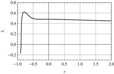
Figure 3: Lyapunov exponent of the map (3) for Singer’s function (9).

Let us first consider Singer’s function Jackson

$$f(x)=7.86x-23.31x^{2}+28.75x^{3}-13.3x^{4},$$ (9)

and the map $f_{r}$ generated from it by means of (3). Since $f(x)$ has a positive Schwarzian derivative in a subinterval of $[0,1]$, exactly the same happens with $f_{r}(x)$. However, a numerical computation of the Lyapunov exponent shows that $f_{r}(x)$ has robust chaos after the origin becomes unstable at $r\approx-0.88156$. In Fig. 3 we can see that the maximum value of the Lyapunov coefficient is in this case $\lambda_{\mathrm{max}}\approx 0.62$, i.e., somewhat smaller than the maximum value $\ln 2$ obtained in all previous examples. As happens in those examples, there is no attractor as the generic orbit wanders chaotically around the whole interval.

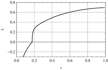
Figure 4: Lyapunov exponent of the map (10) for the logistic map.

We have also explored the one-parameter family of maps

$$f_{r}(x)\equiv\left(\frac{f(x)}{f(c)}\right)^{r},\qquad(r>0),$$ (10)

for some choices of $f(x)$.

In the case of the logistic map $f(x)=x(1-x)$, the map $f_{r}(x)$ is S-unimodal only when $r=1$. For $r>1$ the function has a minimum at the origin. In consequence, $x=0$ is a stable fixed point that attracts the generic orbit, after a chaotic transient, which may be very long for values of $r$ just above 1, for then the basin of attraction of $x=0$ is tiny. For $0<r<1$ the Schwarzian derivative is positive near the origin and $x=1$. For instance,

$$\operatorname{S}f_{r}(x)\sim\frac{1-r^{2}}{2x^{2}}\quad\mbox{as }x\to 0.$$ (11)

Furthermore, the map is not even $C^{3}$ in that case, because its first derivative goes to infinity at $x=0,\ 1$. However, we can see in Fig. 4 that robust chaos arises after the fixed point located in the interval $(1/2,1)$ becomes unstable at $r\approx 0.1759$. The maximum Lyapunov exponent is again $\ln 2$ and is reached at $r=1$, when we recover the logistic map $f(x)=4x(1-x)$. Similar results have been obtained with $f(x)=x\left(1-x^{2}\right)$ and $f(x)=\sin\pi x$.

The examples discussed in this section suggest that robust chaos may not be an unusual property of smooth one-dimensional maps, even when the condition of negative Schwarzian derivative is not satisfied.

IV Robust chaos and conjugate maps

All the maps generated here and in previous works have qualitatively similar dynamics: the solution wanders around the whole interval in a chaotic way. Furthermore, the graphs of all the maps $g=f_{r}$ look rather similar: they start from $g(0)=0$, increase monotonically until $g(c)=1$ and the decrease monotonically until $g(1)=0$. This suggest all the maps are conjugate Ott to each other, i.e., given two of these maps, $g$ and $\tilde{g}$, there exist a homeomorphism $\phi$ on $[0,1]$ such that $\tilde{g}=\phi\circ g\circ\phi^{-1}$. In other words, there exists a continuous change of variables $x\to\tilde{x}=\phi(x)$, with continuous inverse, such that

$$\phi\left[g(x)\right]=\tilde{g}\left[\phi(x)\right],\quad\forall x\in[0,1].$$ (12)

The dynamical systems $x_{n+1}=g\left(x_{n}\right)$ and $\tilde{x}_{n+1}=\tilde{g}\left(x_{n}\right)$ have essentially equivalent dynamics (for instance, if the unstable periodic orbits are dense for $g$ the same will happen for $\tilde{g}$). If, additionally, $\phi$ and $\phi^{-1}$ are smooth both maps have the same Lyapunov coefficient Ott .

This property provides a simple method of constructing families of maps with robust chaos and constant Lyapunov exponent: take a chaotic map $f(x)$ and a smooth homeomorphism $\phi(x)$ on $[0,1]$ depending continuously on a parameter $r$. Them $f_{r}\equiv\phi\circ f\phi^{-1}$ will have the same Lyapunov exponent for all values of $r$. For instance, using $f(x)=4x(1-x)$ and $\phi(x)=x^{r}$ for $r>0$ we get

$$f_{r}(x)=4^{r}x\left(1-x^{1/r}\right)^{r},\qquad(r>0),$$ (13)

whose Lyapunov exponent will be $\lambda=\ln 2$ for all $r>0$. However, this is not S-unimodal, except for $r=1$, because its Schwarzian derivative becomes positive near $x=0$ for $r>1$ and near $x=1$ for $0<r<1$. (Moreover, $f_{r}(1)>0$ for $0<r<1$.) We see again that the condition of negative Schwarzian derivative is not conserved by smooth changes of coordinates and is not necessary for robust chaos. Notice that, by using the well known results corresponding to the full logistic map Ott , we can write explicitly the solution of the dynamical system driven by the map (13) as $x_{n}=\sin^{2r}\left(2^{n}\arcsin x_{0}^{1/2r}\right)$ and its natural invariant density as $\rho(x)=\left[\pi^{2}r^{2}x^{2}\left(x^{-1/r}-1\right)\right]^{-1/2}$. The ‘B-Exponential’ map of Ref. Shastry also is conjugate to the logistic map $g(x)=4x(1-x)$.

On the other hand, given two maps, $g$ and $\tilde{g}$, with the qualitative properties mentioned at the start of this section, one can use a method of successive approximations to construct the function $\phi$, if it exists. One may proceed as follows:

$$\phi_{0}(x) = x,$$ (14)

$$\phi_{n+1}(x) = \tilde{g}^{-1}\left[\phi_{n}\left(g(x)\right)\right],\quad(n=0,1,2,\ldots).$$ (15)

The inverse function $\tilde{g}^{-1}$ is two-valued in this kind of map, but the right preimage is given by the condition that if $c$ and $\tilde{c}$ are the critical points of $g$ and $\tilde{g}$ then $\phi(x)>\tilde{c}$ when $x>c$. The method can be checked by computing $\phi^{-1}$ in the same way to make sure that $\tilde{g}$ and $\phi\circ g\circ\phi^{-1}$ agree to the desired accuracy.

Figure 5: Change of variables $\tilde{x}=\phi(x)$ when $\tilde{g}=4x(1-x)$ and $g$ is (16) with $r=10$.

We have found that the method converges quickly when $\tilde{g}(x)=4x(1-x)$ and $g$ is one of the maps generated in Refs. Andrecut1 ; Andrecut2 . For instance, if we choose $g(x)$ as given by the map

$$f_{r}(x)=\frac{1-r^{-x(1-x)}}{1-r^{-1/4}}$$ (16)

of Ref. Andrecut2 , with $r=10$ and $\tilde{g}(x)=4x(1-x)$, we get the result of Figure 5. Similar results are obtained with other values of $r$ and for the map in Ref. Andrecut1 . All these maps are thus conjugate to $f(x)=4x(1-x)$ and, in consequence Ott , to the tent map. Since the function $\phi$ and its inverse are smooth, all these maps share the Lyapunov exponent $\lambda=\ln 2$.

Figure 6: Change of variables $\tilde{x}=\phi(x)$ when $\tilde{g}=4x(1-x)$ and $g$ is (3), with $r=0$ and $f(x)$ is given by (9).

We have checked numerically that also the maps generated from $f(x)=x(1-x)$ by means of the different methods presented in this work are conjugate to $f(x)=4x(1-x)$ and, thus, to the tent map. But there is a crucial difference: although $\phi$ and $\phi^{-1}$ are continuous they are not smooth enough for the two maps to share the same Lyapunov exponent. For instance, in Fig. 6 we have chosen $\tilde{g}=4x(1-x)$ and $g$ as given by (3), with $r=0$, for Singer’s map (9). It is clear there that $\phi^{\prime}(x)$ vanishes at some points and, since the graph of $\phi^{-1}$ is obtained by exchanging the axes of Fig. 6, the derivative of $\phi^{-1}(x)$ is infinite at those points.

This explains why the corresponding Lyapunov exponents are different. From this point of view, one can understand the methods of previous works as an easy way to construct one-parameter families of conjugate maps by means of smooth homeomorphisms that guarantee the conservation of the Lyapunov exponent, while the methods discussed here are easy ways of constructing conjugate maps with Lyapunov exponents varying in a continuous way, since they are conjugated by non-smooth homeomorphisms.

Figure 7: Zoom of a $0.01\times 0.01$ square of Fig. 6.

The complex structure of the graph of $\phi(x)$ in Fig. 6 can be explored by zooming in on small parts of it. For instance, in Fig. 7 one can seen the function in the interval $[0.5,0.51]$. (A similar zoom of Fig. 5 reveals a smooth structure.)

In fact, the graph in Fig. 6, as well as the remaining graphs we have obtained with the maps generated by the methods presented in this work, looks very similar to the graph of Minkowski’s question mark function Minkowski shown in Fig. 8. The resemblance is even more striking when both $g$ and $\tilde{g}$ are symmetric around the point $x=1/2$.

Figure 8: Minkowski’s question mark function.

Minkowski’s $?(x)$ function is continuous with continuous inverse, strictly increasing and its derivative is zero almost everywhere and infinite or undefined otherwise Viader ; Paradis . The question mark function is the homeomorphism $\phi$ conjugating the tent map and the Farey map Panti defined as $g(x)=x/(1-x)$ for $0\leq x\leq 1/2$ and $g(x)=(1-x)/x$ for $1/2\leq x\leq 1$. We have used this fact to check the accuracy of the method of successive approximations given by (14)–(15). The fact that $?(x)$ is not smooth explains the different Lyapunov exponents of the tent map ($\tilde{\lambda}=\ln 2$) and the Farey map ($\lambda=0$). It also explains why the natural invariant density of the latter map is not normalizable: $\rho(x)\propto x^{-1}$.

The numerical evidence we have found and the dependence on the parameter of the Lyapunov coefficient strongly support the conjecture that the functions $\phi$ conjugating pairs of maps generated by the methods described in this work are not differentiable at an infinite number of points, probably almost everywhere.

On the other hand, the fact that Minkowski’s question mark function can be recursively constructed by using the Farey sequence and continuity Girgensohn suggests an alternative method to construct $\phi$ for functions $g$ and $\tilde{g}$. One starts from the critical point $x_{0}=c$, since we know $y_{0}\equiv\phi(x_{0})=\phi(c)=\tilde{c}$. Then for each pair $(x_{n},y_{n}\equiv\phi(x_{n}))$ already computed, one can calculate two new pairs

$$\left(x_{n+1},\ y_{n+1}\equiv\phi\left(x_{n+1}\right)\right)=\left(g^{-1}_{\pm}\left(x_{n}\right),\ \tilde{g}^{-1}_{\pm}\left(y_{n}\right)\right),$$ (17)

where $g^{-1}_{-}(x)$ is the value $y$ satisfying $g(y)=x$ and $y\leq c$, while $y=g^{-1}_{+}(x)$ is given by the conditions $g(y)=x$ and $y>c$. Analogous definitions are used for $\tilde{g}^{-1}_{\pm}$. We have checked that applying recursively (17) one obtains again Figs. 6 and 7. The method also works for other pairs of maps constructed by means of (3), (8) or (10).

V Final comments

In previous examples —including those of Refs. Andrecut1 ; Andrecut2 but excluding (13)— the maximum is located at the same point for all values of $r$; but this is not a necessary condition. Let us consider the one-parameter family of maps

$$f_{r}(x)\equiv\frac{f\left(x^{r}\right)}{f(c)},\qquad(0<r\leq 1),$$ (18)

which is obtained from family (10) by means of the smooth homeomorphism $\phi(x)=x^{1/r}$. For instance, if $f(x)=x(1-x)$, the maximum of (18) is located at $x=\phi(1/2)=2^{-1/r}$ and the Lyapunov exponent is that of Fig. 4 and its maximum value $\ln 2$ is reached again when $r=1$ and we recover the full logistic map $f_{1}(x)=4x(1-x)$.

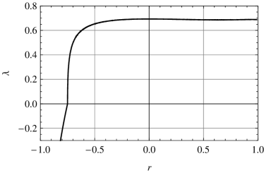
Figure 9: Lyapunov exponent of the map (19) for the logistic map.

We have also considered the following family of maps:

$$f_{r}(x)\equiv\frac{f\left[(1+r)x-rx^{2}\right]}{f(c)},\qquad(-1\leq r\leq 1).$$ (19)

If $f(x)=x(1-x)$, the maximum is located at $x=\left(\sqrt{1+r^{2}}-1+r\right)/(2r)$ and the origin becomes unstable for $r=-3/4$. Again the maximum Lyapunov coefficient is $\ln 2$, but it remains very close to this value for a large parameter interval, as shown in Fig. 9.

In all the examples considered above, as well as in those of Refs. Andrecut1 ; Andrecut2 , the Lyapunov exponent is never higher than $\ln 2$; but it is easy to get other maximum values by changing the starting map $f(x)$. Let consider only a simple example. The piecewise linear map

$$g(x)\equiv\begin{cases}3x,&\mbox{if }0\leq x\leq 1/3;\\ 2-3x;&\mbox{if }1/3\leq x\leq 2/3;\\ 3x-2,&\mbox{if }2/3\leq x\leq 1\end{cases}$$ (20)

has $\left|g^{\prime}(x)\right|=3$, except at $x=1/3,\ 2/3$. In consequence, its Lyapunov exponent is $\ln 3$ and its natural invariant density $\rho(x)=1$. If we use the change of variables $\tilde{x}=\phi(x)\equiv\sin^{2}(\pi x/2)$, the conjugate map $f\equiv\phi\circ g\circ\phi^{-1}$ is

$$f(x)=x(4x-3)^{2}.$$ (21)

The Lyapunov exponent of $f$ is $\ln 3$, because $\phi$ is smooth. Since $\phi$ is precisely the map conjugating the tent map and the full logistic map $g(x)=4x(1-x)$, the natural invariant density of the later is also that of $f$.

Although this map is qualitatively different from those considered above (for instance, it has two critical points), the Lyapunov coefficient of the corresponding family (3) looks much like that in Fig. 1, except for the fact that the origin becomes unstable at $r=-8/9$ and that the maximum value at $r=0$ is now $\lambda_{\mathrm{max}}=\ln 3$. If one computes the homeomorphism conjugating two maps of the family by a trivial extension of the method (14)–(15), one obtains a graph similar to that of Fig. 6. The same happens if one uses family (10), in which case the Lyapunov coefficient is similar to that of Fig. 4, with the bifurcation at $r=1/9$ and the maximum value at $r=1$ given again by $\lambda_{\mathrm{max}}=\ln 3$.

For other values of the maximum Lyapunov exponent one can use a similar method starting from a piecewise linear map with the desired value of the Lyapunov exponent. On the other hand, if a constant Lyapunov exponent is needed, we can use instead the method leading to (13) but starting from an appropriate chaotic map, such as (21).

- (1) E. Ott, Chaos in Dynamical Systems, 2nd. Ed. (Cambridge, Cambridge, 2002), Chap. 2.
- (2) S. Hayes, C. Grebogi and E. Ott, Phys. Rev. Lett. 70, 3031 (1993).
- (3) S. Banerjee, J. A. Yorke and C. Grebogi, Phys. Rev. Lett. 80, 3049 (1998).
- (4) E. Barreto, B. R. Hunt, C. Grebogi and J. A. Yorke, Phys. Rev. Lett. 78, 4561 (1997).
- (5) M. Andrecut and M. K. Ali, Europhys. Lett. 54, 300 (2001).
- (6) M. Andrecut and M. K. Ali, Phys. Rev. E 64, 025203(R) (2001).
- (7) D. Singer, SIAM J. Appl. Math. 35, 260 (1978).
- (8) E. A. Jackson, Perspectives of nonlinear dynamics, Vol. 1 (Cambridge, Cambridge, 1991). Appendix D.
- (9) M. C Shastry, N. Nagaraj and P. G. Vaidya, “The B-Exponential Map: A Generalization of the Logistic Map and its Applications in Generating Pseudo-Random Numbers,” arXiv:cs.CR/0607069 (2006).
- (10) W. de Melo and S. van Strien, Bull. Am. Math. Soc. 18, 159 (1988).
- (11) H. Minkowski, Verhandlungen des III. Internationalen Mathematiker-Kongresses in Heidelberg, (Berlin, 1904).
- (12) P. Viader, J. Paradís and L. Bibiloni, J. Number Theory 73, 212 (1998).
- (13) J. Paradís, P. Viader and L. Bibiloni, J. Math. Anal. Appl. 253, 107 (2001).
- (14) G. Panti, Monatsh. Math. 154, 247 (2008).
- (15) R. Girgensohn, J. Math. Anal. Appl. 203, 127 (1996).