Large forward-backward asymmetry in $B\to K\mu^{+}\mu^{-}$
from new physics tensor operators

Abstract

We study the constraints on possible new physics contribution to the forward-backward asymmetry of muons, $A_{FB}(q^{2})$, in $B\rightarrow K\mu^{+}\mu^{-}$. New physics in the form of vector/axial-vector operators does not contribute to $A_{FB}(q^{2})$ whereas new physics in the form of scalar/pseudoscalar operators can enhance $A_{FB}(q^{2})$ only by a few per cent. However new physics the form of tensor operators can take the peak value of $A_{FB}(q^{2})$ to as high as $40\%$ near the high-$q^{2}$ end point. In addition, if both scalar/pseudoscalar and tensor operators are present, then $A_{FB}(q^{2})$ can be more than $15\%$ for the entire high-$q^{2}$ region $q^{2}>15$ GeV². The observation of significant $A_{FB}$ would imply the presence of new physics tensor operators, whereas its $q^{2}$-dependence could further indicate the presence of new scalar/pseudoscalar physics.

I Introduction

Flavor changing neutral interactions (FCNI) are forbidden at the tree level in the standard model (SM). Therefore they have the potential to test higher order corrections to the SM and also constrain many of its possible extensions. Among all FCNI, rare $B$ decays play an important role in searching new physics beyond the SM. The quark level FCNI $b\to s\mu^{+}\mu^{-}$ is responsible for (i) the inclusive semileptonic decay $B\to X_{s}\mu^{+}\mu^{-}$, (ii) the exclusive semileptonic decays $B\to(K,K^{*})\mu^{+}\mu^{-}$, and (iii) the purely leptonic decay $B_{s}\rightarrow\mu^{+}\mu^{-}$. Both the inclusive and exclusive semileptonic decays have been observed experimentally babar04_incl ; belle05_incl ; babar-03 ; babar-06 ; belle-03 ; hfag with branching ratios close to their SM predictions ali-02 ; lunghi ; kruger-01 ; isidori .

In alok-sankar01 , the impact of these measurement on the new physics contribution to the branching ratio $B(B_{s}\rightarrow\mu^{+}\,\mu^{-})$ was considered. It was shown that new physics in the form of vector/axial-vector operators is severely constrained by the data on $B(B\rightarrow K\mu^{+}\mu^{-})$ and $B(B\rightarrow K^{*}\mu^{+}\mu^{-})$, so an order of magnitude enhancement in the branching ratio of $B_{s}\rightarrow\mu^{+}\mu^{-}$ is ruled out. On the other hand, if new physics is in the form of scalar/pseudoscalar operators, then $B(B\to K^{*}\mu^{+}\mu^{-})$ does not put any useful constraint on the new physics couplings and allows an order of magnitude enhancement in the $B(B_{s}\rightarrow\mu^{+}\,\mu^{-})$. Therefore $B(B_{s}\rightarrow\mu^{+}\mu^{-})$ is sensitive to an extended Higgs sector. In tension , the constraints on scalar/pseudoscalar new physics contribution to the $B(B\rightarrow K\mu^{+}\mu^{-})$ were studied. It was shown that a large deviation in $B(B\rightarrow K\mu^{+}\,\mu^{-})$ from its SM prediction is not possible.

In ali-92 , the forward-backward (FB) asymmetry of leptons in semileptonic decays of mesons was introduced as an observable sensitive to the physics beyond the SM. In particular, the FB asymmetry of muons, $A_{FB}$, in $B\rightarrow K\mu^{+}\,\mu^{-}$ is important because its value is negligibly small in the SM ali-00 . This is due to the fact that hadronic current for $B\rightarrow K$ transition does not have any axial vector contribution; it can have a nonzero value only if it receives contribution from new physics. The sensitivity of $A_{FB}$ for testing non-standard Higgs sector has been studied in literature in detail yan-00 ; bobeth-01 ; erkol-02 ; demir-02 ; li-04 . However in alok-02 , it was shown that the present upper bound on the branching ratio of $B_{s}\rightarrow\mu^{+}\mu^{-}$ cdf-07 restricts the average (or integrated) FB asymmetry, $\left\langle A_{FB}\right\rangle$, to about $1\%$ as long as the only new physics is in the form of scalar/pseudoscalar operators. Such a small FB asymmetry is very difficult to be measured in experiments and hence searching for new scalar/pseudoscalar physics through $\left\langle A_{FB}\right\rangle$ will be a futile exercise.

The forward-backward asymmetry can also get contributions from tensor operators. In the SM, the tensor operators in $b\to s\mu^{+}\mu^{-}$ arise at higher order in the electroweak operator product expansion from finite external momenta in the matching calculations, however their contribution is negligibly small and we shall not consider them in this paper. However in models beyond the SM, tensor operators may contribute significantly to the decay and to the asymmetry $A_{FB}$. For example, in the minimal supersymmetric standard model (MSSM), the tensor operators arise from photino and zino box diagrams at the leading order operator product expansion Bobeth:2007dw . Tensor operators can also be induced by scalar operators under renormalization group running Hiller:2003js ; Borzumati:1999qt . In leptoquark models, tensor operators are induced by the interactions of leptoquarks with the SM Higgs field Hirsch:1996qy .

In Bobeth:2007dw , the effect of these operators to $\left\langle A_{FB}\right\rangle$ was studied, where it was shown that $\left\langle A_{FB}\right\rangle$ can be as high as $3\%$ at $90\%$ C.L. if new physics is only in the form of tensor operators, whereas it can rise to $15\%$ if both scalar/pseudoscalar and tensor new physics operators are present. The integrated asymmetry $\left\langle A_{FB}\right\rangle$ has been measured by BaBar babar-06 and Belle belle-06 ; ikado-06 to be

$$\left\langle A_{FB}\right\rangle=(0.15_{-0.23}^{+0.21}\pm 0.08)\,\,\,\,\,\,{\rm(BaBar)}\,,$$ (1)

$$\left\langle A_{FB}\right\rangle=(0.10\pm 0.14\pm 0.01)\,\,\,\,{\rm(Belle)}.$$ (2)

These measurements are consistent with zero. However, they can be as high as $\sim 40\%$ within $2\sigma$ error bars. Future experiments like a Super-$B$ factory or the LHC will increase the statistics by more than two orders of magnitude. For example at ATLAS, the number of expected $B\rightarrow K\mu^{+}\,\mu^{-}$ events even after analysis cuts is expected to be $\sim 4000$ with $30$ fb^-1 data Adorisio , which will be collected within the first three years. Thus, $\langle A_{FB}\rangle$ can soon be probed to values as low as $5\%$.

With higher statistics, one will be able to determine even the distribution of $A_{FB}$ as a function of the invariant dilepton mass squared $q^{2}$, which can provide a stronger handle on this quantity than just its average value $\langle A_{FB}\rangle$. Moreover, since the theoretical predictions for the rate of $B\rightarrow K\mu^{+}\,\mu^{-}$ are rather uncertain in the intermediate $q^{2}$ region ($7$ GeV${}^{2}<q^{2}<12$ GeV²) owing to the vicinity of charmed resonances, it is important to look at the quantity $A_{FB}(q^{2})$ in the complete $q^{2}$ range so that its robust features may be identified. Indeed, it turns out that with the new physics considered in this paper, $A_{FB}(q^{2})$ is high near the high-$q^{2}$ end point.

In this paper we study $A_{FB}(q^{2})$ in the complete $q^{2}$ region and explore the possibility of large FB asymmetry in some specific regions of the dilepton invariant mass spectrum. This paper is organized as follows. In section II, we present the theoretical expressions for the FB asymmetry of $B\rightarrow K\mu^{+}\,\mu^{-}$ considering new physics in the form of scalar/pseudoscalar and tensor operators. In section III we study $A_{FB}(q^{2})$ due to new physics only in the form of scalar/pseudoscalar operators whereas in section IV we consider $A_{FB}(q^{2})$ due to new physics only in the form of tensor operators. In section V, we calculate $A_{FB}(q^{2})$ when both the scalar/pseudoscalar we well as tensor operators are present. Finally in section VI, we present the conclusions.

II Forward-backward asymmetry of muons in $B\rightarrow K\mu^{+}\,\mu^{-}$

We consider new physics in the form of scalar/pseudoscalar and tensor operators. The effective Lagrangian for the quark level transition $b\rightarrow s\mu^{+}\mu^{-}$ can be written as

$$L(b\rightarrow s\mu^{+}\mu^{-})=L_{SM}+L_{SP}+L_{T}\;,$$ (3)

where

$$L_{SM} = \frac{\alpha G_{F}}{\sqrt{2}\pi}V_{tb}V^{\star}_{ts}\biggl{\{}C^{\rm eff}_{9}(\bar{s}\gamma_{\mu}P_{L}b)\,\bar{\mu}\gamma_{\mu}\mu+C_{10}(\bar{s}\gamma_{\mu}P_{L}b)\,\bar{\mu}\gamma_{\mu}\gamma_{5}\mu$$ (4)

$$-2\frac{C^{\rm eff}_{7}}{q^{2}}m_{b}\,(\bar{s}i\sigma_{\mu\nu}q^{\nu}P_{R}b)\,\bar{\mu}\gamma_{\mu}\mu\biggr{\}}\;,$$

$$L_{SP} = \frac{\alpha G_{F}}{\sqrt{2}\pi}V_{tb}V^{\star}_{ts}\biggl{\{}R_{S}~{}\bar{s}P_{R}b~{}\bar{\mu}\mu+R_{P}~{}\bar{s}P_{R}b\,\bar{\mu}\gamma_{5}\mu\biggr{\}}\;,$$ (5)

$$L_{T} = \frac{\alpha G_{F}}{\sqrt{2}\pi}V_{tb}V^{\star}_{ts}\biggl{\{}C_{T}~{}\bar{s}\sigma_{\mu\nu}b~{}\bar{\mu}\sigma^{\mu\nu}\mu+iC_{TE}~{}\bar{s}\sigma_{\mu\nu}b~{}\bar{\mu}\sigma_{\alpha\beta}\mu~{}\epsilon^{\mu\nu\alpha\beta}\biggr{\}}\;.$$ (6)

Here $P_{L,R}=(1\mp\gamma_{5})/2$ and $q_{\mu}$ is the sum of 4-momenta of $\mu^{+}$ and $\mu^{-}$. $R_{S}$ and $R_{P}$ are new physics scalar/pseudoscalar couplings whereas $C_{T}$ and $C_{TE}$ are new physics tensor couplings.

Within the SM, the Wilson coefficients in eq. (4) have the following values:

$$C_{7}^{\rm eff}=-0.310\;,\;C_{9}^{\rm eff}=+4.138+Y(q^{2})\;,\;C_{10}=-4.221\;,$$ (7)

where the function $Y(q^{2})$ is given by buras-95 ; misiak-95

$$Y(q^{2}) = g(m_{c},q^{2})(3C_{1}+C_{2}+3C_{3}+C_{4}+3C_{5}+C_{6})-\frac{1}{2}g(0,q^{2})(C_{3}+3C_{4})$$ (8)

$$- \frac{1}{2}g(m_{b},q^{2})(4C_{3}+4C_{4}+3C_{5}+C_{6})+\frac{2}{9}(3C_{3}+C_{4}+3c_{5}+C_{6})\;.$$

Here we take the values of the relevant Wilson coefficients to be

$$C_{1}=-0.249,\ C_{2}=1.107,\ C_{3}=0.011,$$

$$C_{4}=-0.025,\ C_{5}=0.007,\ C_{6}=-0.031,$$ (9)

all of which are computed at the scale $\mu=m_{b}=5$ GeV. The function $g$ is given by

$$g(m_{i},q^{2})=-\frac{8}{9}\ln(m_{i}/m_{b}^{\text{pole}})+\frac{8}{27}+\frac{4}{9}y_{i}-\frac{2}{9}(2+y_{i})\sqrt{|1-y_{i}|}$$ (10)

$$\times\left\{\Theta(1-y_{i})\left[\ln\left(\frac{1+\sqrt{1-y_{i}}}{1-\sqrt{1-y_{i}}}\right)-i\pi\right]+\Theta(y_{i}-1)\ 2\tan^{-1}\left(\frac{1}{\sqrt{y_{i}-1}}\right)\right\},$$

with $y_{i}\equiv 4m_{i}^{2}/q^{2}$.

The normalized FB asymmetry is defined as

$$A_{FB}(z)=\frac{\int_{0}^{1}dcos\theta\frac{d^{2}\Gamma}{dz\ dcos\theta}-\int_{-1}^{0}dcos\theta\frac{d^{2}\Gamma}{dz\ dcos\theta}}{\int_{0}^{1}dcos\theta\frac{d^{2}\Gamma}{dz\ dcos\theta}+\int_{-1}^{0}dcos\theta\frac{d^{2}\Gamma}{dz\ d\cos\theta}}\;.$$ (11)

with $z\equiv q^{2}/m_{B}^{2}$. In order to calculate the FB asymmetry, we first need to calculate the differential decay width. The decay amplitude for $B(p_{1})\to K(p_{2})\,\mu^{+}(p_{+})\,\mu^{-}(p_{-})$ is given by

$$M\,(B\rightarrow K\mu^{+}\mu^{-}) = \frac{\alpha G_{F}}{2\sqrt{2}\pi}V_{tb}V^{\star}_{ts}$$ (12)

$$\times \Bigg{[}\left<K(p_{2})\left|\bar{s}\gamma_{\mu}b\right|B(p_{1})\right>\left\{C_{9}^{\rm eff}\bar{u}(p_{-})\gamma_{\mu}v(p_{+})+C_{10}\bar{u}(p_{-})\gamma_{\mu}\gamma_{5}v(p_{+})\right\}$$

$$-2\frac{C^{\rm eff}_{7}}{q^{2}}m_{b}\left<K(p_{2})\left|\bar{s}i\sigma_{\mu\nu}q^{\nu}b\right|B(p_{1})\right>\;\bar{u}(p_{-})\gamma_{\mu}v(p_{+})$$

$$+\left<K(p_{2})\left|\bar{s}b\right|B(p_{1})\right>\;\left\{R_{S}\bar{u}(p_{-})v(p_{+})+R_{P}\bar{u}(p_{-})\gamma_{5}v(p_{+})\right\}$$

$$+2C_{T}\left<K(p_{2})\left|\bar{s}\sigma_{\mu\nu}b\right|B(p_{1})\right>\;\bar{u}(p_{-})\sigma^{\mu\nu}v(p_{+})$$

$$+2iC_{TE}\epsilon^{\mu\nu\alpha\beta}\left<K(p_{2})\left|\bar{s}\sigma_{\mu\nu}b\right|B(p_{1})\right>\;\bar{u}(p_{-})\sigma_{\alpha\beta}v(p_{+})\Bigg{]}\;,$$

where $q_{\mu}=(p_{1}-p_{2})_{\mu}=(p_{+}+p_{-})_{\mu}$. The relevant matrix elements are

$$\left<K(p_{2})\left|\bar{s}\gamma_{\mu}b\right|B(p_{1})\right> = (2p_{1}-q)_{\mu}f_{+}(z)+(\frac{1-k^{2}}{z})\,q_{\mu}[f_{0}(z)-f_{+}(z)]\;,$$ (13)

$$\left<K(p_{1})\left|\bar{s}i\sigma_{\mu\nu}q^{\nu}b\right|B(p_{1})\right> = \Big{[}(2p_{1}-q)_{\mu}q^{2}-(m_{B}^{2}-m_{K}^{2})q_{\mu}\Big{]}\,\frac{f_{T}(z)}{m_{B}+m_{K}}\;,$$ (14)

$$\left<K(p_{2})\left|\bar{s}b\right|B(p_{1})\right> = \frac{m_{B}(1-k^{2})}{\hat{m}_{b}}f_{0}(z)\;,$$ (15)

$$\left<K(p_{2})\left|\bar{s}\sigma_{\mu\nu}b\right|B(p_{1})\right> = -i\Big{[}(2p_{1}-q)_{\mu}q_{\nu}-(2p_{1}-q)_{\nu}q_{\mu}\Big{]}\,\frac{f_{T}}{m_{B}+m_{K}}\;,$$ (16)

where $k\equiv m_{K}/m_{B}$ and $\hat{m}_{b}\equiv m_{b}/m_{B}$.

Using the above matrix elements, the double differential decay widths can be calculated as

$$\frac{d^{2}\Gamma}{dzdcos\theta} = \frac{G_{F}^{2}\alpha^{2}}{2^{11}\pi^{5}}\,|V_{tb}V_{ts}^{*}|^{2}\,m_{B}^{5}\,\phi^{1/2}$$ (17)

$$\times \Bigg{[}z\left\{\frac{\hat{m}_{\mu}}{m_{B}}{\rm Re}(CE^{*})+\frac{1}{4m_{B}^{2}}(|E|^{2}+\beta_{\mu}^{2}|D|^{2})\right\}$$

$$+\phi\left\{\frac{1}{4}(|A|^{2}+|B|^{2})\,+\,2\hat{m}_{\mu}\,m_{B}\,{\rm Re}(AF^{*})\right\}$$

$$+(1-k^{2})\left\{2\hat{m}_{\mu}^{2}{\rm Re}(BC^{*})+\frac{\hat{m}_{\mu}}{m_{B}}{\rm Re}(BE^{*})\right\}$$

$$+\hat{m}_{\mu}^{2}\left\{(2+2k^{2}-z)|B|^{2}+z|C|^{2}\right\}+\phi\,z\,m_{B}^{2}\,(1-\beta_{\mu}^{2})|F|^{2}$$

$$+\phi\beta_{\mu}^{2}\left\{z\,m_{B}^{2}(|F|^{2}+4|G|^{2})-\frac{1}{4}(|A|^{2}+|B|^{2})\right\}\cos^{2}\theta$$

$$-\Bigg{.}\phi^{1/2}\beta_{\mu}\left\{\frac{\hat{m}_{\mu}}{m_{B}}{\rm Re}(AD^{*})+4m_{\mu}(1-k^{2}){\rm Re}(BG^{*})+4z\hat{m}_{\mu}m_{B}{\rm Re}(CG^{*})\right.\Bigg{.}$$

$$+\left.\Bigg{.}2z{\rm Re}(GE^{*})+\frac{z}{4}{\rm Re}(DF^{*})\right\}\Bigg{.}\cos\theta\Bigg{]}\;,$$

where

$$\hat{m}_{\mu} \equiv m_{\mu}/m_{B}$$

$$\phi \equiv 1+k^{4}+z^{2}-2(k^{2}+k^{2}z+z)\;,$$

$$\beta_{\mu} \equiv \sqrt{1-\frac{4\hat{m}_{\mu}^{2}}{z}}\;,$$ (18)

and $\theta$ is the angle between the momenta of $K$ meson and $\mu^{-}$ in the dilepton centre of mass frame. The parameters $A,B,C,D,E,F,G$ are combinations of the Wilson coefficients and the form factors, given by

$$A \equiv 2C^{eff}_{9}\,f_{+}(z)-4C^{eff}_{7}\hat{m}_{b}\frac{f_{T}(z)}{1+k}\;,$$

$$B \equiv 2C_{10}\,f_{+}(z)\;,$$

$$C \equiv 2C_{10}\,\frac{1-k^{2}}{z}\Big{[}f_{0}(z)-f_{+}(z)\Big{]}\;,$$

$$D \equiv 2R_{S}\frac{m_{B}(1-k^{2})}{\hat{m}_{b}}f_{0}(z)\;,$$

$$E \equiv 2R_{P}\frac{m_{B}(1-k^{2})}{\hat{m}_{b}}f_{0}(z)\;,$$

$$F \equiv -4C_{T}\frac{f_{T}(z)}{m_{B}(1+k)}\;,$$

$$G \equiv 4C_{TE}\frac{f_{T}(z)}{m_{B}(1+k)}\;.$$ (19)

The kinematical variables in eq. (17) are bounded as

$$-1\leq\cos\theta\leq 1,\;\;4\hat{m}^{2}_{\mu}\leq z\leq(1-k)^{2}\;.$$ (20)

The form factors $f_{+,\,0,\,T}$ can be calculated in the light cone QCD approach. Their $z$ dependence is given by ali-00

$$f(z)=f(0)\,\exp(c_{1}z+c_{2}z^{2}+c_{3}z^{3})\;,$$ (21)

where the parameters $f(0),c_{1}$, $c_{2}$ and $c_{3}$ for each form factor are given in Table 1.

$$\begin{array}[]{l c c c c}\hline\cr&\phantom{-}f(0)&\phantom{-}c_{1}&\phantom{-}c_{2}&\phantom{-}c_{3}\\ \hline\cr f_{+}&\phantom{-}0.319^{+0.052}_{-0.041}&\phantom{-}1.465&\phantom{-}0.372&\phantom{-}0.782\\ f_{0}&\phantom{-}0.319^{+0.052}_{-0.041}&\phantom{-}0.633&\phantom{-}-0.095&\phantom{-}0.591\\ f_{T}&\phantom{-}0.355^{+0.016}_{-0.055}&\phantom{-}1.478&\phantom{-}0.373&\phantom{-}0.700\\ \hline\cr\end{array}$$

Table 1: Form factors for the $B\to K$ transition ali-00 .

The FB asymmetry arises from the $\cos\theta$ term in the last two lines of eq. (17). We get

$$A_{FB}(z)=\frac{2\Gamma_{0}\,\beta_{\mu}\,\phi\,N(z)}{d\Gamma/dz}\;,$$ (22)

where

$$\Gamma_{0}=\frac{G_{F}^{2}\alpha^{2}}{2^{12}\pi^{5}}|V_{tb}V^{*}_{ts}|^{2}m_{B}^{5}\;,$$ (23)

$$N(z) = -4m_{\mu}(1-k^{2}){\rm Re}(BG^{*})-\frac{\hat{m}_{\mu}}{m_{B}}{\rm Re}(AD^{*})-4z\hat{m}_{\mu}m_{B}{\rm Re}(CG^{*})$$ (24)

$$-\frac{z}{4}{\rm Re}(DF^{*})-2z{\rm Re}(EG^{*})\;,$$

$$\frac{d\Gamma}{dz} = \Gamma_{0}\,\phi^{1/2}\times\Bigg{[}\phi\left(1-\frac{1}{3}\beta_{\mu}^{2}\right)\,(|A|^{2}+|B|^{2})\,+\,4\,\hat{m}_{\mu}^{2}\,|B|^{2}\,(2+2k^{2}-z)\,+\,4\,\hat{m}_{\mu}^{2}\,z\,|C|^{2}\,$$ (25)

$$+\,8\,\hat{m}_{\mu}^{2}\,(1-k^{2})\,{\rm Re}(BC^{*})\,+\,8\hat{m}_{\mu}\,m_{B}\phi\,{\rm Re}(AF^{*})\,+\,\frac{z}{m_{B}^{2}}\,(|E|^{2}+\beta_{\mu}^{2}\,|D|^{2})$$

$$+\frac{4\hat{m}_{\mu}}{m_{B}}\,(1-k^{2})\,{\rm Re}(BE^{*})+\frac{4\hat{m}_{\mu}}{m_{B}}\,z\,{\rm Re}(CE^{*})$$

$$+\,\frac{4}{3}\,\phi\,z\,m_{B}^{2}\,\left\{3|F|^{2}\,+\,2\,\beta_{\mu}^{2}\,(2|G|^{2}-|F|^{2})\,\right\}\Bigg{]}\;.$$

In our analysis we assume that there are no additional CP phases apart from the single Cabibbo-Kobayashi-Maskawa (CKM) phase. Under this assumption the new physics couplings are all real.

III $A_{FB}$ from new scalar/pseudoscalar operators

If new physics is only in the form of scalar/pseudoscalar operators, then $A_{FB}(z)$ is obtained by putting $C_{T}=C_{TE}=0$ in eq. (12). We get

$$A_{FB}(z)=\frac{\beta_{\mu}\,\phi^{1/2}\,a_{SM,S}(z)\,R_{S}}{b_{SM}(z)\,+\,b_{SM,S}(z)R_{P}\,+\,b_{S}(z)(R_{S}^{2}+R_{P}^{2})}\;,$$ (26)

where

$$a_{SM,S}(z) = -\frac{4\hat{m}_{\mu}}{\hat{m}_{b}}\,(1-k^{2})\,f_{0}(z)\,{\rm Re}(A)\;,$$ (27)

$$b_{SM}(z) = \phi\left(1-\frac{1}{3}\beta_{\mu}^{2}\right)\,(|A|^{2}+|B|^{2})\,+\,4\,\hat{m}_{\mu}^{2}\,|B|^{2}\,(2+2k^{2}-z)$$ (28)

$$+\,4\,\hat{m}_{\mu}^{2}\,z\,|C|^{2}\,+\,8\,\hat{m}_{\mu}^{2}\,(1-k^{2})\,{\rm Re}(BC^{*})\;,$$

$$b_{SM,S}(z) = \,\frac{16\hat{m}_{\mu}}{\hat{m}_{b}}(1-k^{2})^{2}\,C_{10}\,f_{0}^{2}(z)\;,$$ (29)

$$b_{S}(z) = \frac{4\,z}{\hat{m}_{b}^{2}}(1-k^{2})^{2}\,f_{0}^{2}(z)\;.$$ (30)

Therefore in order to estimate $A_{FB}(z)$ we need to know the scalar/pseudoscalar couplings $R_{S}$ and $R_{P}$.

We constrain $R_{S}$ and $R_{P}$ through the decay $B_{s}\rightarrow\mu^{+}\,\mu^{-}$. The branching ratio of $B_{s}\rightarrow\mu^{+}\,\mu^{-}$ due to $L_{SM}+L_{SP}$ is given by alok-02

$$B(B_{s}\rightarrow\mu^{+}\,\mu^{-})=\frac{G_{F}^{2}\,\alpha^{2}\,m_{B_{s}}^{3}\,\tau_{B_{s}}}{64\pi^{3}}|V_{tb}V_{ts}^{*}|^{2}\,f_{B_{s}}^{2}\times\left[R_{S}^{2}+\left(R_{P}\,+\,2\hat{m}_{\mu}\,C_{10}\right)^{2}\right]\;.$$ (31)

The present upper bound on $B(B_{s}\rightarrow\mu^{+}\,\mu^{-})$ is cdf-07

$$B(B_{s}\rightarrow\mu^{+}\mu^{-})<0.58\times 10^{-7}\quad(95\%~{}{\rm C.L.})\;,$$ (32)

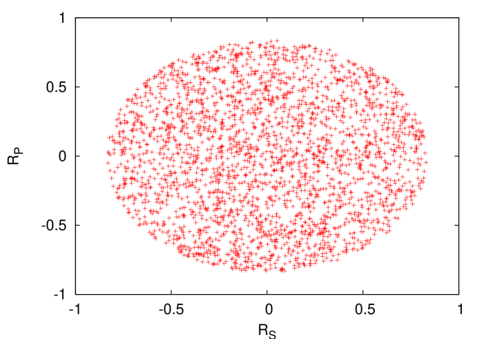
which is still more than an order of magnitude away from its SM prediction. Therefore we will neglect the SM contribution while obtaining constraints on the $R_{S}-R_{P}$ parameter space. The allowed values of $R_{S}$ and $R_{P}$ at $2\sigma$ are shown in Fig. 1. The input values of parameters, used throughout this paper, are given in Table 2.

Figure 1: $R_{S}-R_{P}$ parameter space allowed by the present upper bound on the branching ratio of $B_{s}\rightarrow\mu^{+}\,\mu^{-}$

$$G_{F}=1.166\times 10^{-5}\;{\rm GeV}^{-2}$$

beneke-99

charles

ali-02

ali-02 Aubert:2004aw

Table 2: Numerical inputs used in our analysis. Unless explicitly specified, they are taken from the Review of Particle Physics Yao:2006px .

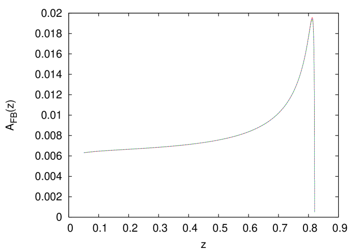
The maximum value of $A_{FB}(z)$ is obtained for $R_{P}=0$ and $R_{S}=\pm 0.84$. At these parameter values, $A_{FB}(z)$ is shown in Fig. 2 for the central and $\pm 2\sigma$ values of the form factors. As can be observed, the errors in the form factors have almost no impact on the value of $A_{FB}(z)$ obtained. The peak value of $A_{FB}(z)$ is observed to be $\approx 2\%$, whereas in most of the $z$ range, $A_{FB}(z)<1\%$. Measurement of $A_{FB}(z)$ in the presence of only scalar/pseudoscalar operators will therefore be very challenging.

Figure 2: The forward-backward asymmetry $A_{FB}(z=q^{2}/m_{B}^{2})$ for the new physics only in the form of scalar/pseudoscalar operators. The plot corresponds to $R_{P}=0$ and $R_{S}=-0.84$. The red (solid) curve corresponds to the central values of the the form factors given in Table 1 whereas the green (dashed) and blue (dotted) curves correspond to their values at $+2\sigma$ and $-2\sigma$ respectively. In this scenario, all the curves overlap, indicating that the dependence on form factors is negligibly small.

IV $A_{FB}$ from new tensor operators

If new physics is only in the form of tensor operators then $A_{FB}(z)$ is obtained by putting $R_{S}=R_{P}=0$ in eq. (12). We get

$$A_{FB}(z)=\frac{\beta_{\mu}\,\phi^{1/2}\,a_{SM,T}(z)\,C_{TE}}{b_{SM}(z)\,+\,b_{SM,T}(z)C_{T}\,+\,b_{T}(z)(C_{T}+4C_{TE}^{2})}\;,$$ (33)

where

$$a_{SM,T}(z) = -64\,\hat{m}_{\mu}\,(1-k)\,C_{10}\,f_{T}(z)\,f_{0}(z)\;,$$ (34)

$$b_{SM,T}(z) = -\,\frac{32\,\hat{m}_{\mu}\,\phi\,{\rm Re}(A)\,f_{T}(z)}{1+k}\;,$$ (35)

$$b_{T}(z) = \frac{64\,\phi\,z\,f_{T}^{2}(z)}{3\,(1+k)^{2}}\;,$$ (36)

and $b_{SM}(z)$ is given already in eq. (28).

In order to estimate $A_{FB}(z)$, we need to know the tensor couplings $C_{T}$ and $C_{TE}$. In alok-03 , it was shown that the the most stringent bound on tensor couplings comes from the data on the branching ratio of the inclusive decay $B\rightarrow X_{s}\mu^{+}\,\mu^{-}$. The branching ratio of $B\to X_{s}(p_{s})\mu^{+}(p_{\mu^{+}})\mu^{-}(p_{\mu^{-}})$ is given by fukae

$$B(B\to X_{s}l^{+}l^{-})=B_{0}\Bigg{[}I_{SM}+(C_{T}^{2}+4C_{TE}^{2})I_{T}\Bigg{]}\,,$$ (37)

where

$$I_{SM} = \int dz\,\Bigg{[}\frac{8u(z)}{z}\left\{1-z^{2}+\frac{1}{3}u(z)^{2}\right\}C_{7}^{\rm eff}$$ (38)

$$-2\,u(z)\left\{z^{2}+\frac{1}{3}u(z)^{2}-1\right\}({C_{9}^{\rm eff}}^{2}+C_{10}^{2})$$

$$-16\,u(z)\,(z-1)\,C_{9}^{\rm eff}\,C_{7}^{\rm eff}\Bigg{]}\;,$$

$$I_{T} = 16\int dz\,u(z)\Bigg{[}\frac{-2}{3}u(z)^{2}-2z+2\Bigg{]}\;,$$ (39)

$$u(z) = (1-z)\;.$$ (40)

Here $z\equiv q^{2}/m_{b}^{2}=(p_{\mu^{+}}+p_{\mu^{-}})^{2}/m_{b}^{2}=(p_{b}-p_{s})^{2}/m_{b}^{2}$. The limits of integration for $z$ are now

$$z_{min}=4m_{\mu}^{2}/{m_{b}}^{2}\;,\quad z_{max}=(1-\frac{m_{s}}{m_{b}})^{2}\;,$$ (41)

as opposed to the ones given in eq. (20) for the exclusive decay. The normalization factor $B_{0}$ is given by

$$B_{0}=B(B\to X_{c}e\nu)\frac{3\alpha^{2}}{16\pi^{2}}\frac{|V_{ts}^{*}V_{tb}|^{2}}{|V_{cb}|^{2}}\frac{1}{f(\hat{m_{c}})\kappa(\hat{m_{c}})}\;,$$ (42)

where the phase space factor $f(\hat{m_{c}}={m_{c}\over m_{b}})$, and the $O(\alpha_{s})$ QCD correction factor $\kappa(\hat{m_{c}})$ of $b\rightarrow ce\nu$ are given by Kim

$$f(\hat{m_{c}}) = 1-8\hat{m_{c}}^{2}+8\hat{m_{c}}^{6}-\hat{m_{c}}^{8}-24\hat{m_{c}}^{4}\ln\hat{m_{c}}\;,$$ (43)

$$\kappa(\hat{m_{c}}) = 1-\frac{2\alpha_{s}(m_{b})}{3\pi}\left[(\pi^{2}-\frac{31}{4})(1-\hat{m_{c}})^{2}+\frac{3}{2}\right]\;.$$ (44)

Eq. (37) can be written as

$$B(B\rightarrow X_{s}\mu^{+}\,\mu^{-})=B_{SM}(B\rightarrow X_{s}\mu^{+}\,\mu^{-})+B_{T}(B\rightarrow X_{s}\mu^{+}\,\mu^{-})\;,$$ (45)

where

$$B_{SM}(B\rightarrow X_{s}\mu^{+}\,\mu^{-}) = B_{0}\,I_{SM}\;,$$ (46)

$$B_{T}(B\rightarrow X_{s}\mu^{+}\,\mu^{-}) = B_{0}\,I_{T}\,(C_{T}^{2}+4C_{TE}^{2})\;.$$ (47)

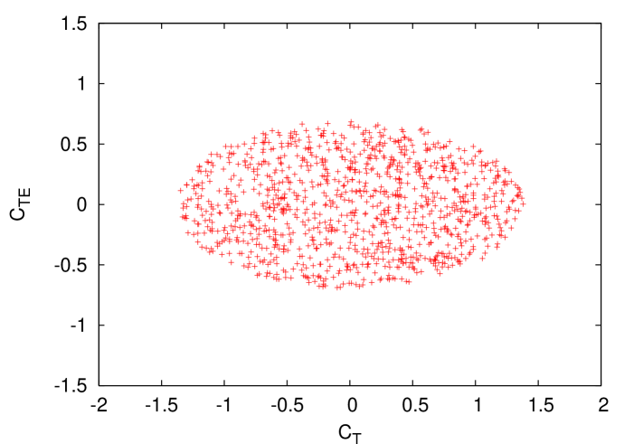
Figure 3: $(C_{T},C_{TE})$ parameter space at $2\sigma$ allowed by the measurement of branching ratio of $B\rightarrow X_{s}\mu^{+}\,\mu^{-}$

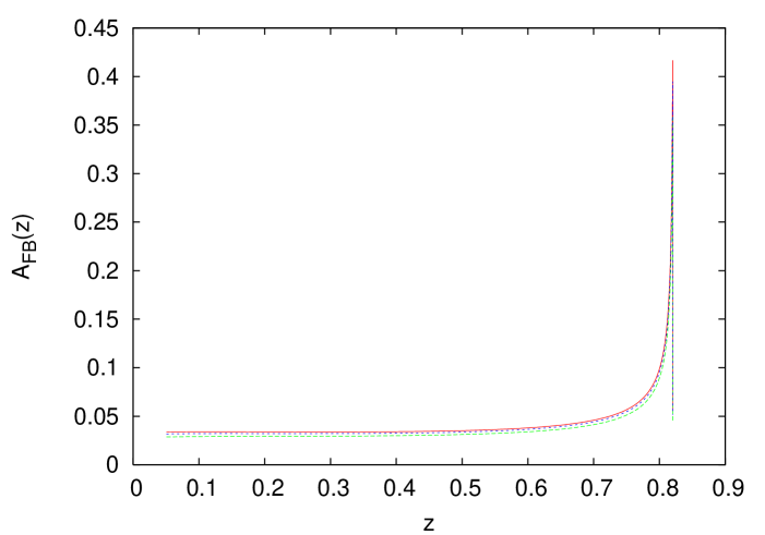
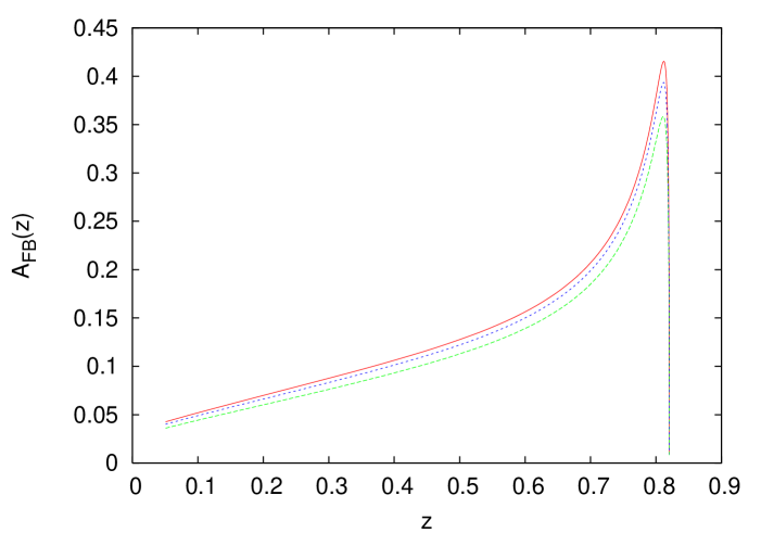
Figure 4: The forward-backward asymmetry $A_{FB}(z=q^{2}/m_{B}^{2})$ for the new physics only in the form of tensor operators. The plot corresponds to $C_{T}=0$ and $C_{TE}=+0.69$. The red (solid) curve corresponds to the central values of the the form factors given in Table 1 whereas the green (dashed) and blue (dotted) curves correspond to their values at $+2\sigma$ and $-2\sigma$ respectively. The dependence on the form factors is clearly extremely small.

The present world average for $B(B\rightarrow X_{s}\mu^{+}\,\mu^{-})$ is hfag

$$B_{\rm Exp}(B\rightarrow X_{s}\mu^{+}\,\mu^{-})_{q^{2}>0.04\,{\rm GeV^{2}}}=(4.3^{+1.3}_{-1.2})\times 10^{-6}\;.$$ (48)

We keep the same invariant mass cut, $q^{2}>0.04$ GeV², in order to enable comparison with the experimental data. With this range of $q^{2}$, the SM branching ratio for $B\rightarrow X_{s}\mu^{+}\,\mu^{-}$ in NNLO is ali-02

$$B_{SM}(B\rightarrow X_{s}\mu^{+}\,\mu^{-})_{q^{2}>0.04\,{\rm GeV^{2}}}=(4.15\pm 0.71)\times 10^{-6}\;,$$ (49)

whereas $B_{0}I_{T}=(1.47\pm 0.22)\times 10^{-6}$. Using equations (45), (48) and (49), we get

$$C_{T}^{2}+4C_{TE}^{2}=0.10\pm 1.01\;.$$ (50)

The allowed parameter space for $C_{T},C_{TE}$ at $2\sigma$ is shown in Fig. 3.

The maximum value of $A_{FB}(z)$ is obtained for $C_{T}=0$ and $C_{TE}=\pm 0.69$. For these parameter values, $A_{FB}(z)$ is shown in Fig. 4 for the central and $\pm 2\sigma$ values of the form factors. In most of the $z$ range, $A_{FB}(z)\mathrel{\hbox{\hbox to0.0pt{\hbox{\lower 4.0pt\hbox{$\sim$}}\hss}\hbox{$<$}}}3\%$, however its peak value at the high-$q^{2}$ end point is $\sim 40\%$. Thus there can be a large deviation from the SM prediction in the high-$q^{2}$ region.

V $A_{FB}$ from the combination of scalar/pseudoscalar and tensor operators

Figure 5: The forward-backward asymmetry $A_{FB}(z=q^{2}/m_{B}^{2})$ for new physics when both scalar/pseudoscalar as well as tensor operators are present. The plot corresponds to $R_{S}=C_{T}=0$ and $R_{P}=-0.84,\,C_{TE}=+0.69$. The red (solid) curve corresponds to the central values of the the form factors given in Table 1 whereas the green (dashed) and blue (dotted) curves correspond to their values at $+2\sigma$ and $-2\sigma$ respectively.

We now consider the scenario where new physics in the form of both scalar/pseudoscalar and tensor operators are present. In this case the expression for $A_{FB}(z)$ is given by eq. (12). Maximum values of $A_{FB}(z)$ as obtained for $R_{S}=C_{T}=0$ and $R_{P}=-0.84,\,C_{TE}=0.69$, which are shown in Fig. 5. The peak value of $A_{FB}(z)$ is $\sim 40\%$ at $2\sigma$ and is obtained at the high-$q^{2}$ end point. Thus, there can be large FB asymmetry in the high $q^{2}$ region. Another reason to concentrate on the high-$q^{2}$ region is that theoretical predictions of the decay rate $B\rightarrow K\mu^{+}\,\mu^{-}$ are more robust there, owing to the non-interference of charmed resonances.

Let ${\cal R}$ be the high-$q^{2}$ region, with $q_{0}<q^{2}<q^{2}_{\rm max}$, where $q^{2}_{\rm max}$ is the endpoint. The restriction to high-$q^{2}$ would decrease the number of events selected, however since the average $A_{FB}$ in this region, $\langle A_{FB}^{\cal R}\rangle$, is larger, it can still be observed. The number of events of $B\rightarrow K\mu^{+}\,\mu^{-}$ required to determine this asymmetry to $n\sigma$ is

$$N_{B\rightarrow K\mu^{+}\,\mu^{-}}\mathrel{\hbox{\hbox to0.0pt{\hbox{\lower 4.0pt\hbox{$\sim$}}\hss}\hbox{$>$}}}\frac{n^{2}}{\langle A_{FB}^{\cal R}\rangle^{2}f^{\cal R}}\;,$$ (51)

where $f^{\cal R}$ is the fraction of total number of $B\rightarrow K\mu^{+}\,\mu^{-}$ events that lie in the region ${\cal R}$. When ${\cal R}$ corresponds to the whole $q^{2}$ range available, then the expression reduces to $N_{B\rightarrow K\mu^{+}\,\mu^{-}}\mathrel{\hbox{\hbox to0.0pt{\hbox{\lower 4.0pt\hbox{$\sim$}}\hss}\hbox{$>$}}}n^{2}/\langle A_{FB}\rangle^{2}$, as expected.

Taking ${\cal R}$ to be the region $q^{2}>15$ GeV² and the values of parameters as shown in Fig. 5, we find that about 600 total $B\rightarrow K\mu^{+}\,\mu^{-}$ events are required to observe FB asymmetry at $2\sigma$. For $q^{2}>19$ GeV², the required number of events for $2\sigma$ detection of $A_{FB}$ is about 1600. These numbers are easily obtainable at a Super-$B$ factory as well as at the LHC, so the structure of the $A_{FB}(q^{2})$ peak can be studied at these experiments.

VI Conclusions

In the standard model, the forward-backward asymmetry $A_{FB}$ of muons in $B\rightarrow K\mu^{+}\mu^{-}$ is negligible. New physics in the form of vector/axial vector operators also cannot contribute to $A_{FB}$. However, new physics in the form of scalar/pseudoscalar or tensor operators can enhance $A_{FB}$ to per cent level or more, thus bringing it within the reach of the LHC or a Super-$B$ factory. In this paper, we concentrate on the magnitude as well as $q^{2}$ dependence of $A_{FB}$ with these kinds of new physics.

We find that if new physics is in the form of scalar/pseudoscalar operators only, then the peak value of $A_{FB}(q^{2})$ can only be $\mathrel{\hbox{\hbox to0.0pt{\hbox{\lower 4.0pt\hbox{$\sim$}}\hss}\hbox{$<$}}}2\%$, and hence rather challenging to detect. However if new physics is only in the form of tensor operators then the peak value of $A_{FB}(q^{2})$ can be as high as $40\%$. Such a high enhancement is obtained only near the high-$q^{2}$ end point, i.e. for $q^{2}>19$ GeV², below which $A_{FB}(q^{2})\mathrel{\hbox{\hbox to0.0pt{\hbox{\lower 4.0pt\hbox{$\sim$}}\hss}\hbox{$<$}}}5\%$. In the presence of both scalar/pseudoscalar and tensor operators, the interference terms between them can boost $A_{FB}(q^{2})$ to more than $15\%$ for the whole region $q^{2}>15$ GeV².

The measurement of the distribution of $A_{FB}$ as a function of $q^{2}$ can not only reveal new physics, but also indicate its possible Lorentz structure. A large enhancement in $A_{FB}$ by itself would confirm the presence of new physics tensor operators. If the enhancement is only at large $q^{2}$ values, the scalar/pseudoscalar new physics operators probably play no major role. On the other hand, if the enhancement as a function of $q^{2}$ is significant at low $q^{2}$ and increases gradually with increasing $q^{2}$, the presence of scalar/pseudoscalar new physics operators would be indicated.

The high-$q^{2}$ region in the $A_{FB}(q^{2})$ distribution is theoretically clean since the charmed resonances in the intermediate $q^{2}$ region do not interfere here. This region also happens to be highly sensitive to new physics, especially in the form of tensor operators, as we have shown here. Exploration of this region in the upcoming experiments is therefore of crucial importance.