Top Quark Mass Measurement Using a Matrix Element Method with Quasi–Monte Carlo Integration

Abstract

We report an updated measurement of the top quark mass obtained from $p\bar{p}$ collisions at $\sqrt{s}=1.96$ TeV at the Fermilab Tevatron using the CDF II detector. Our measurement uses a matrix element integration method to obtain a signal likelihood, with a neural network used to identify background events and a likelihood cut applied to reduce the effect of badly reconstructed events. We use a 2.7 fb^-1 sample and observe 422 events passing all of our cuts. We find $m_{t}$ = 172.2 $\pm$ 1.0 (stat.) $\pm$ 0.9 (JES) $\pm$ 1.0 (syst.) GeV/$c^{2}$, or $m_{t}$ = 172.2 $\pm$ 1.7 (total) GeV/$c^{2}$.

I INTRODUCTION

The top quark is the heaviest known particle in the Standard Model. Its mass is an important parameter to be determined, both for its intrinsic interest, and because precision measurements of the top quark mass, in conjunction with the $W$ boson mass, allow us to set constraints on the mass of the Higgs boson within the Standard Model. In this letter we describe a precision measurement of the top quark mass using a matrix element integration method. This measurement uses 2.7 fb^-1 of data collected by the CDF II detector.

We obtain a top mass measurement by integrating over unmeasured quantities in the matrix element using a quasi–Monte Carlo integration. This allows us to minimize assumptions made about the kinematics of an event, resulting in improved precision. The integration method yields a likelihood curve as a function of the top pole mass.

The largest source of systematic uncertainty in our measurement is the jet energy scale (JES). To reduce our uncertainty due to this source, we introduce an additional parameter to our likelihood, $\Delta_{\mathop{\mathrm{JES}}}$, which allows us to use the information in the $W$ decay to determine the JES. $\Delta_{\mathop{\mathrm{JES}}}$ parameterizes the shift in JES in units of the systematic error for a given jet. Our likelihood is thus constructed as a 2D function of $m_{t}$ and $\Delta_{\mathop{\mathrm{JES}}}$; we then combine the likelihoods for all events and eliminate $\Delta_{\mathop{\mathrm{JES}}}$ as a nuisance parameter to find a final top mass value.

II EVENT SELECTION

At the Fermilab Tevatron, top quarks are predominantly produced in $t\bar{t}$ pairs, where the $t$ decays into a $W$ boson and a $b$ quark $\sim$ 100% of the time. The $W$ can then decay into a charged lepton and a neutrino (“leptonic” decay) or a quark-antiquark pair (“hadronic” decay). We search for events in the “lepton + jets” channel, where one $W$ decays hadronically and one leptonically. Thus, we analyze events with four high-energy jets (two from the $b$ quarks and two from the hadronic $W$ decay), at least one of which is required to be $b$-tagged using a secondary vertex algorithm which identifies tracks displaced from the primary vertex; exactly one high energy electron or muon (from the leptonic $W$ decay); and large missing transverse energy (from the neutrino).

The principal backgrounds to our signal are events where a $W$ boson is produced in conjunction with heavy flavor jets ($b\bar{b}$, $c\bar{c}$, or $c$), a $W$ boson is produced with light jets which are mistagged as $b$-jets, and QCD events not containing a $W$ where the $W$ signature is faked. Overall we expect 105.7 $\pm$ 42.0 background events in our observed 494 candidate events. Table 1 shows our expected backgrounds.

Table 1: Expected backgrounds for the $W$+4 tight jet sample used.

Background	1 tag	$\geq$ 2 tags
non-W QCD	20.0 $\pm$ 17.3	0.8 $\pm$ 1.6
W+light mistag, diboson, or $Z$	27.7 $\pm$ 5.6	1.1 $\pm$ 0.1
W+heavy ($b\bar{b}$, $c\bar{c}$, $c$)	45.0 $\pm$ 37.8	6.0 $\pm$ 5.0
Single top	3.8 $\pm$ 0.2	1.2 $\pm$ 0.2
Total background	96.5 $\pm$ 36.8	9.2 $\pm$ 5.2
Predicted top signal	259.4 $\pm$ 33.6	98.8 $\pm$ 16.0
Events observed	389	105

III MATRIX ELEMENT METHOD

We calculate a two-dimensional likelihood as a function of $m_{t}$ and $\Delta_{\mathop{\mathrm{JES}}}$ by integrating over the matrix element for $t\bar{t}$ production and decay over the unknown parton-level quantities, using transfer functions to connect these with the measured jets. Our overall likelihood formula is:

$$L(\vec{y}\mid m_{t},\Delta_{\mathop{\mathrm{JES}}})=\frac{1}{N(m_{t})}\frac{1}{A(m_{t},\Delta_{\mathop{\mathrm{JES}}})}\sum_{i\,=1}^{24}w_{i}L_{i}(\vec{y}\mid m_{t},\Delta_{\mathop{\mathrm{JES}}})$$ (1)

with

$$L_{i}(\vec{y}\mid m_{t},\Delta_{\mathop{\mathrm{JES}}})=\int\frac{f(z_{1})f(z_{2})}{FF}~{}\textrm{TF}(\vec{y}\mid\vec{x},\Delta_{\mathop{\mathrm{JES}}})~{}|M(m_{t},\vec{x})|^{2}~{}d\Phi(\vec{x}),$$ (2)

where $\vec{x}$ denotes the parton-level quantities, $\vec{y}$ denotes the quantities measured in our detector, $M$ is the matrix element for $t\bar{t}$ production and decay, $f(z)$ is the parton distribution functions (PDFs) for the momenta of the two incoming particles, FF is the flux factor normalizing the PDFs, $N(m_{t})$ is a normalization factor, $A(m_{t},\Delta_{\mathop{\mathrm{JES}}})$ is an acceptance factor to correct for the effect of the event selection criteria, and $\Phi$ is the parton-level phase space integrated over. The integral is evaluated for each of the 24 possible jet-parton assignments and then summed with appropriate weights corresponding to the probability that a given jet-parton assignment corresponds with the observed $b$-tags. We integrate over a total of 19 variables. In order to perform this integral in a practical amount of time, we employ quasi–Monte Carlo integration qmc , which uses quasi-random sequences. These sequences provide more uniform coverage of the phase space, resulting in faster integral convergence than with normal Monte Carlo techniques.

We use a neural network to identify events likely to be background, and subtract out their contribution to the total likelihood by estimating the average contribution for background events from Monte Carlo. We also consider the effect of events which we call “bad signal”. These are events which contain an actual $t\bar{t}$ decay, but where the final observed objects in our detector do not come directly from $t\bar{t}$ decay (due to extra jets from initial or final state radiation, $W\rightarrow\tau$ decay, or other causes). To reduce the effect of these poorly-modeled events, we apply a cut of 10 to the peak of the log-likelihood curve. In Monte Carlo simulation, this cut eliminates 20% of “bad signal” events and 27% of background while retaining 97% of our good signal events.

We test and calibrate our measurement using pythia Monte Carlo events over a variety of input $m_{t}$ and $\Delta_{\mathop{\mathrm{JES}}}$ values by performing pseudo-experiments. Using the results of the pseudo-experiments, we obtain a final set of calibration constants for our measured top mass and statistical uncertainty. Figure 1 shows the results of our Monte Carlo testing. Figure 2 shows the effect of the likelihood cut on Monte Carlo events.

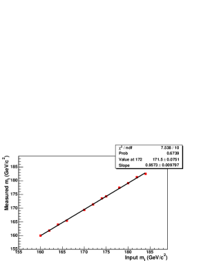
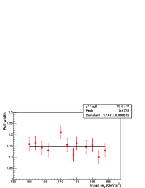
Figure 1: Results using Monte Carlo events to test and calibrate our method. Left: measured mass vs. input mass. Right: pull width vs. input mass.

IV RESULT

We have 494 events passing our initial selection cuts, of which 422 events pass the likelihood cut as well. With these 422 events, we measure:

$m_{t}$ = 172.2 $\pm$ 1.0 (stat.) $\pm$ 0.9 (JES) $\pm$ 1.0 (syst.) GeV/$c^{2}$ = 172.2 $\pm$ 1.7 (total) GeV/$c^{2}$

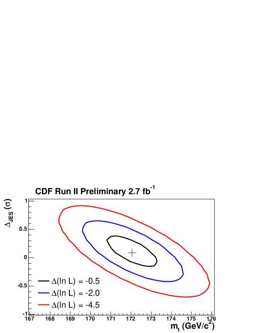
Figure 2: Left: Value of the log-likelihood curve at its peak for good signal, bad signal, and background events in Monte Carlo. The dashed line shows the cut at 10 used. Right: Contours of the 2D likelihood distributions obtained with our final data sample. The contours shown correspond to a statistical uncertainty of 1, 2, and 3 $\sigma$.

Figure 2 shows the final contours of 1-$\sigma$, 2-$\sigma$, and 3-$\sigma$ statistical uncertainty around the measured value. The total result attains a precision of better than 1% in $m_{t}$.

Our main sources of systematic uncertainty are from the Monte Carlo generator used for our calibration and testing (0.5 GeV/$c^{2}$), the residual JES uncertainty resulting from variation of the individual sources of our total JES uncertainty (0.5 GeV/$c^{2}$), uncertainty from the modeling of the jet energy scale for $b$-jets (0.4 GeV/$c^{2}$), and uncertainty in the background model (0.4 GeV/$c^{2}$). We also have smaller uncertainties from initial-state and final-state radiation, lepton $P_{T}$ measurement, pileup events, calibration, and PDFs (0.3, 0.2, 0.2, 0.1, and 0.1 GeV/$c^{2}$, respectively), for a total of 1.0 GeV/$c^{2}$.

- (1) H. Neiderreiter, Random Number Generation and Quasi-Monte Carlo Methods (SIAM, Philadelphia, 1992).
- (2) The CDF Collaboration, “Top Mass Measurement in the Lepton + Jets Channel Using a Matrix Element Method with Quasi-Monte Carlo Integration and in situ Jet Calibration with 2.7 fb-1”, CDF public note 9427 (July 2008).