$B_{s}^{0}$ mixing at D0 experiment

Abstract

In this report, we present a preliminary measurement of the ${B_{s}^{0}}$ mixing parameter using samples of four partially reconstructed semileptonic $B_{s}^{0}$ decays and one fully reconstructed hadronic decay mode, corresponding to approximately 2.4 $fb^{-1}$ of integrated luminosity. We perform an unbinned likelihood fit to the proper decay length and obtain $\Delta m_{s}=18.53\pm 0.93(\rm stat.)\pm 0.30({\rm syst.})~{}ps^{-1}$.

I INTRODUCTION

Particle-antiparticle oscillations are observed and well established in the $B_{d}^{0}$ system. The mass difference ${\Delta{m}_{d}}$ is measured to be ${\Delta{m}_{d}}=0.507\pm 0.005$ ps^-1 pdg . $B_{s}^{0}$ mesons are known to oscillate with a high frequency according to standard model predictions. Observing the oscillations in the $B_{s}^{0}$ system has been an important focus of the B physics program at both the D0 and the CDF experiments at Tevatron. D0 reported direct limits on the ${B_{s}^{0}}$ mixing parameter ${\Delta{m}_{s}}$ bsmixd0 using the ${B_{s}^{0}\to D_{s}^{-}\mu^{+}\nu X}$, ${D_{s}^{-}\rightarrow\phi\pi^{-}}$ decay mode . CDF reported a measurement of this parameter exceeding 5 $\sigma$ significance bsmixcdf . The measurement of this parameter is an important test of the CKM (Cabibbo Kobayashi Maskawa) formalism of the standard model, and combining it with a measurement of ${\Delta{m}_{d}}$ allows us to reduce the error on $V_{td}$ and constrain one side of the CKM triangle. This report describes the measurement of the $B_{s}^{0}$ mixing parameter at the D0 experiement using 2.4 $fb^{-1}$ of data with 3 $\sigma$ significance.

We use the central tracker, muon chambers and calorimeters to reconstruct the $B$ decays. Details of the detector can be found elsewhere d0det . We use a single inclusive muon trigger or a di-muon trigger to accumulate samples for ${B_{s}^{0}}$ mixing studies. In the case of di-muon trigger the other muon acts as the tag muon used to identify the flavor of the $B$ meson which we discuss later. The trigger requires a good muon identified by the muon chamber with a matching track in the central tracker in the pseudo-rapidity range of $|\eta|<2.0$. The triggers use $p_{T}$ cuts between $3-5$ ${{\rm GeV}/c}$ and the trigger is prescaled or turned off depending on the luminosity. Hence for the ${B_{s}^{0}\to D_{s}^{-}e^{+}\nu X}$ decay mode, and the hadronic decay mode, we are using a tagged sample with the muon acting as a tag.

II $B_{s}^{0}$ DECAYS SAMPLE SELECTION AND RECONSTRUCTION

D0 reported direct limits on $B_{s}^{0}$ oscillations using the decay mode ${B_{s}^{0}\to D_{s}^{-}\mu^{+}\nu X}$ decays with ${D_{s}^{-}\rightarrow\phi\pi^{-}}$ bsmixd0 . In this report, we present a preliminary measurement of the $B_{s}^{0}$ oscillations bsmixd0meas , using four additional decay modes. We use three additional semileptonic decay modes namely ${B_{s}^{0}\to D_{s}^{-}e^{+}\nu X}$, with ${D_{s}^{-}\rightarrow\phi\pi^{-}}$ and ${B_{s}^{0}\to D_{s}^{-}\mu^{+}\nu X}$ decays with ${D_{s}^{-}\rightarrow K^{\ast 0}K^{-}}$, $K^{\ast 0}\rightarrow K^{+}\pi^{-}$ (The $K^{\ast 0}$ and the $\phi$ candidates are required to be consistent with known mass and width pdg of these two resonances) and ${D_{s}^{-}\rightarrow K_{S}K^{-}}$. We also use a fully reconstructed hadronic mode, namely, ${B_{s}^{0}\to D_{s}^{-}\pi^{+}+X}$ decay, with ${D_{s}^{-}\rightarrow\phi\pi^{-}}$.

${B_{s}^{0}}$ decays are identified in their semileptonic modes, both in muon and electron mode. Muons are required to have $p_{T}>1.5{{\rm GeV}/c}$, and to be in the pseudo-rapidity region of $|\eta|<2.0$. Electrons are required to have $p_{T}>2.0$ ${{\rm GeV}/c}$ and are identified in a pseudo-rapidity region of $|\eta|<1$. The $D_{s}^{-}$ and $B_{s}^{0}$ decay products are constrained to originate from a common vertex and the $B_{s}^{0}$ and $D_{s}^{-}$ decay vertices are required to be significantly displaced from the $p\bar{p}$ collision vertex.

The $K^{\ast 0}\rightarrow K^{+}\pi^{-}$ decay mode requires special treatment on account of large reflections, as both real physics processes and combinatorial background contribute to the signal peak. The peak is comprised of the signal mode, ${D_{s}^{-}\rightarrow K^{\ast 0}K^{-}}$, $K^{\ast 0}\rightarrow K^{+}\pi^{-}$, the physics processes, $D^{+}\rightarrow K^{-}\pi^{+}\pi^{+}$ or $D^{+}\rightarrow K^{\ast 0}\pi^{+}(K^{\ast 0}\rightarrow K^{+}\pi^{-})$, $\Lambda_{c}^{+}\rightarrow K^{+}\pi^{-}p^{+}$, $D^{+}\rightarrow K^{\ast 0}K^{+}(K^{\ast 0}\rightarrow K^{+}\pi^{-})$ (Cabibbo suppressed) and combinatorial background. We fit for these contributions in an unbinned likelihood fit. Fig. 1 shows the fit to the mass distribution of the $M_{K\pi K}$ system with the individual contributions superimposed.

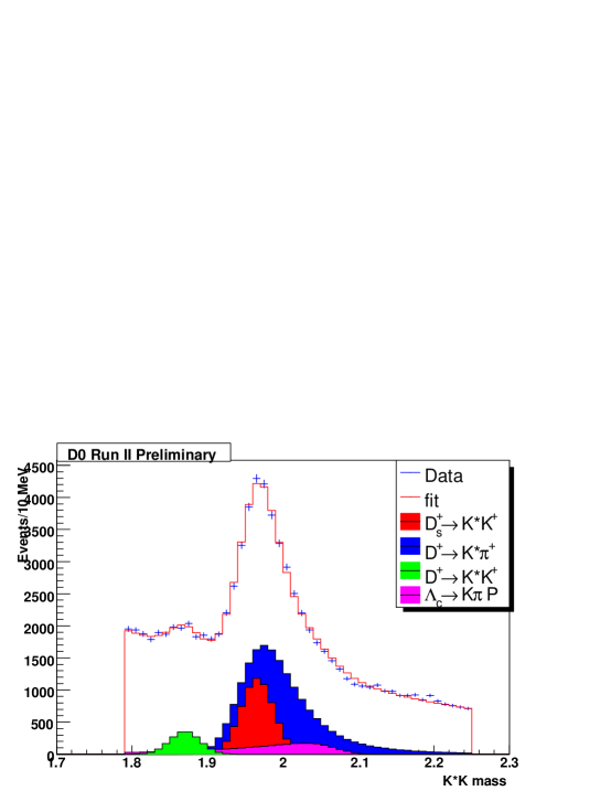
Figure 1: The $M_{(K\pi)K}$ invariant mass distribution where $D_{s}\rightarrow K^{\ast 0}K$ for ${B_{s}^{0}\to D_{s}^{-}\mu^{+}\nu X}$ decay mode

III FLAVOR TAGGING

The flavor of the initial state of the ${B_{s}^{0}}$ is determined using a likelihood ratio method, based on the properties of the other b-hadron in the event (opposite side tagging) and the properties of the particles produced in assosciation with the reconstructed $B_{s}^{0}$ meson (same side tagging) and we then combine the OST and the SST taggers. The performance of any tagger is characterized by its efficiency defined as $\varepsilon=N_{tag}/N_{tot}$ (where $N_{tag}$ is the number of tagged $B_{s}^{0}$ mesons and $N_{tot}$ is the total reconstructed $B_{s}^{0}$ mesons), and the dilution ${\cal{D}}$ which is defined as ${\cal{D}}=\frac{N_{RS}-N_{WS}}{N_{tag}}$ (where $N_{RS}$ and $N_{WS}$ are the right-sign and wrong-sign tags respectively).

The OST is calibrated using $B\rightarrow\mu+\nu D^{\ast-}$ data events, and we obtain the dilution ${\cal{D}}$ as a function of a tag variable $d$ (whose sign indicates a $b$ or $\bar{b}$, and its value indicates the “$b$”-ness of the tag), to provide an event-by-event “predicted” dilution which is used in the unbinned likelihood fit described in section IV. More details on the development of the OST and results can be found in bdmixd0 . The total OST effective tagging power of $\varepsilon{\cal{D}}^{2}=(2.48\pm 0.21^{+0.08}_{-0.06})\%$.

The combined tagger is calibrated using decay modes, $B_{s}^{0}\rightarrow J/\psi\phi$ (using both data and MC) and $B_{s}^{0}\rightarrow\mu D_{s}(\phi\pi)$ (using MC only) (See Fig. 2). The total combined tagging power is $\varepsilon{\cal{D}}^{2}=4.49\pm 0.88\%$. More details on the SST and the combined tagger can be found in combtag .

The SST is used by ${B_{s}^{0}\to D_{s}^{-}\mu^{+}\nu X}$, with ${D_{s}^{-}\rightarrow\phi\pi^{-}}$ decay mode only. All the other decay modes use the OST.

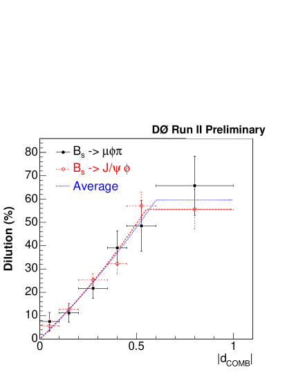
Figure 2: The Combined Tagger dilution calibration

IV UNBINNED LIKELIHOOD FIT AND AMPLITUDE SCAN

IV.1 Visible Proper decay length and scale factor

In semileptonic decays the proper time gets smeared due to the presence of neutrino. To take this into account we introduce a K factor estimated from Monte Carlo (MC) simulation. It is defined as $K=p_{T}(lD_{s})/p_{T}(B)$. The real proper decay length is related to the measured or visible proper decay length ($l_{M}$), by the relation $ct(B_{s}^{0})=l_{M}K$ where $l_{M}=M(B_{s}^{0})\cdot(L_{T})/(p_{T}(lD_{s}))$ is the measured visible proper decay length ($l_{M}$). $L_{T}$ is the distance from the primary vertex to the $B_{s}^{0}$ decay vertex in the transverse plane projected onto the $lD_{s}$ momentum, and $M(B_{s}^{0})$ is the mass of the $B_{s}^{0}$ meson as obtained from PDG pdg .

The $l_{M}$ uncertainty is determined by the vertex fitting procedure, track parameters, and track parameter uncertainties. To account for any imperfections in modeling of detector uncertainties, we use scale factors that are dependent on the topology of hits in the silicon micro-strip tracker to correct the $l_{M}$ uncertainty. These scale factor corrections were obtained from QCD data and MC samples.

IV.2 Likelihood Fit

An unbinned likelihood fit is used to describe and fit for the ${B_{s}^{0}}$ oscillation. All flavor tagged events with $1.72<M(D_{s})<2.22$ ${{\rm GeV}/c^{2}}$ are used in the fit. The probability for oscillated (osc) and non-oscillated (nos) ${B_{s}^{0}}$ decays, as a function of true proper decay length, $x$, can be writtten as

$$p_{s}^{nos}(x)=\frac{K}{c\tau_{B_{s}}}\cdot e^{-\frac{K}{c\tau_{B_{s}}}}\cdot 0.5\cdot(1+{\cal{D}}\cos(\Delta m_{s}\cdot Kx/c))$$ (1)

$$p_{s}^{osc}(x)=\frac{K}{c\tau_{B_{s}}}\cdot e^{-\frac{K}{c\tau_{B_{s}}}}\cdot 0.5\cdot(1-{\cal{D}}\cos(\Delta m_{s}\cdot Kx/c))$$ (2)

The sample is mostly composed of ${B_{s}^{0}}$ decays with some contributions coming from $B_{d}$ and $B_{u}$ mesons also. Similar equations would hold for these decay modes with the oscillatory term getting modified appropriately.

Taking into account momentum uncertainty, and convoluting over detector resolution, the probability for the $j$-th decay mode, as a function of the measured proper decay length, can be written as below :

$$p_{j}^{nos/osc}(x^{M})=\sum_{j}f_{j}(K)dK\epsilon_{j}(x^{M})\int dx~{}g(x-x^{M},x)p_{j}^{nos/osc}(x,K)$$ (3)

$f_{j}(K)$ is the K-factor distribution and we sum over the $K-$ factor bins. $\epsilon_{j}(x^{M})$ is the reconstruction efficiency as a function of lifetime cuts. The fraction of each decay mode contribution is calculated from Monte Carlo. A similar probablity equation holds for the combinatorial background ($p_{bg}$). The background contribution comes from prompt decays with the ${D_{s}^{-}}\mu(e)$ vertex coinciding with the primary vertex, background with fake vertices distributed around the primary vertex, and long lived background.

The likelihood can then be written as follows :

$${\cal{L}}=\prod_{i=1}^{N}((1-f_{sig})p_{i,bg}+f_{sig}p_{i,sig})$$ (4)

.

The amplitude method was first proposed elsewhere amplscan . It involves modifying the likelihood term by introducing an amplitude term ${\cal{A}}$ in front of the oscillatory cosine term, such that,

$${\cal{L}}\propto 1\pm{\cal{A~{}D}}\cos(\Delta m_{s}t)$$ (5)

We minimize $-2ln{\cal L}$ fitting for the parameter ${\cal{A}}$ while ${\cal{D}}$ is known and $\Delta m_{s}$ is varied. The value of ${\Delta{m}_{s}}$ where ${\cal{A}}$ is consistent with 1 and inconsistent with 0 then gives the measurement of the ${\Delta{m}_{s}}$ parameter. All values of ${\Delta{m}_{s}}$ for which ${\cal{A}}+1.645~{}\sigma_{{\cal{A}}}<1$ are excluded at $95\%$ confidence level. The sensitivity of the mixing measurement is defined as the ${\Delta{m}_{s}}$ value for which $1.645~{}\sigma_{{\cal{A}}}=1$.

The combined amplitude scan and the difference between log-likelihood at minimum and elsewhere ($\Delta{\rm ln}{\cal L}$), as a function of $\Delta m_{s}$, can be seen in Fig. 3. $\Delta{\rm ln}{\cal L}$ is derived from the amplitude scan. More details can be found in amplscan .

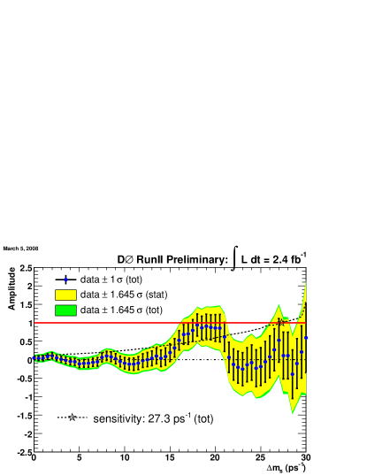
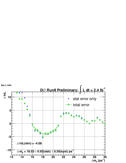
Figure 3: The combined amplitude and likelihood scan.

From a parabolic fit around the minimum of the $\Delta{\rm ln}{\cal L}$ distribution, we obtain $\Delta m_{s}=18.53$ with statistical error of $0.93~{}ps^{-1}$. The systematic error is estimated as $0.3~{}ps^{-1}$, thus giving us a preliminary measurement of $\Delta m_{s}=18.53\pm 0.98~{}ps^{-1}\rm~{}(stat.+syst.)$. From the depth of the likelihood minima, we calculate an overall significance of this measurement as $2.9~{}\sigma$.

References

- (1) W. M. Yao et al., Particle Data Group, J. Phys. G33 (2006)
- (2) V.M. Abazov et al., D0 Collaboration, Phys. Rev. Lett.97, 021802 (2006).
- (3) A. Abulencia et al., CDF Collaboration, Phys. Rev. Lett. 97,242003, (2006).
- (4) V.M. Abazov et al., D0 Collaboration, Nucl. Instrum. and Meth. A565 463-537 (2006).
- (5) D0 Collaboration, Conference Note 5474.
- (6) V.M. Abazov et al., Phys. Rev. D74, 112002 (2006).
- (7) D0 Conference Note 5210.
- (8) H.G. Moser, A. Roussarie, Nucl. Instrum. Meth. A384 491 (1997)