On regularization methods of EM-Kaczmarz type

Abstract

We consider regularization methods of Kaczmarz type in connection with the expectation-maximization (EM) algorithm for solving ill-posed equations. For noisy data, our methods are stabilized extensions of the well established ordered-subsets expectation-maximization iteration (OS-EM). We show monotonicity properties of the methods and present a numerical experiment which indicates that the extended OS-EM methods we propose are much faster than the standard EM algorithm.

Keywords: Ill-posed equations; Regularization; Expectation maximization; Kaczmarz iteration; OS-EM iteration; Integral equations;

AMS Classifications: 65J20, 65J22, 45F05.

1 Introduction

The expectation-maximization (EM) algorithm provides approximations for maximum likelihood estimators of problems with incomplete or noisy data, which is the usual framework when dealing with inverse or ill-posed problems. In particular, the EM algorithm for Poisson models is well known for its applications to astronomical imaging and to PET (positron emission tomography) - see, e.g. [19], [21].

In this work we address inverse problems modeled by operator equations which admit nonnegative solutions, with the aim of approaching them by combined EM-Kaczmarz strategies.

We begin our study by considering the operator equation

$$\operatorname{\mathcal{A}}x=y\,,$$ (1.1)

where $\operatorname{\mathcal{A}}:L^{1}(\Omega)\to L^{1}(\Sigma)$ is a Fredholm integral operator of the first kind

$$(\operatorname{\mathcal{A}}x)(s)\ =\ \int_{\Omega}a(s,t)\,x(t)\,dt,\quad s\in\Sigma\,.$$ (1.2)

Nonnegative solutions of (1.1) can be determined by finding minimizers of the functional

$$f(x)\ :=\ \int_{\Sigma}\Big{[}y(s)\,\ln\frac{y(s)}{(\operatorname{\mathcal{A}}x)(s)}-y(s)+(\operatorname{\mathcal{A}}x)(s)\Big{]}\,ds\,.$$

Formally, the first order necessary condition for such a minimizer reads as

$$\operatorname{\mathcal{A}}^{*}\Big{(}\frac{y}{\operatorname{\mathcal{A}}x}\Big{)}\ =\ \operatorname{\mathcal{A}}^{*}1\,.$$ (1.3)

If the assumption $(\operatorname{\mathcal{A}}^{*}1)(t)=1$ is satisfied, a solution of (1.3) can be obtained by solving the corresponding multiplicative fixed-point equation

$$x\operatorname{\mathcal{A}}^{*}\Big{(}\frac{y}{\operatorname{\mathcal{A}}x}\Big{)}\ =\ x\,.$$ (1.4)

The fixed-point equation (1.4) motivates the definition of the EM algorithm, see [19, 21, 3, 9, 14, 13, 16, 18],

$$x_{k+1}(t)\ =\ x_{k}(t)\ \operatorname{\mathcal{A}}^{*}\Big{(}\frac{y}{\operatorname{\mathcal{A}}x_{k}}\Big{)}(t)=\ x_{k}(t)\ \int_{\Sigma}\frac{a(s,t)y(s)}{(\operatorname{\mathcal{A}}x_{k})(s)}\,ds\,,$$ (1.5)

i.e. an explicit iterative method for solving (1.4).

The OS-EM (ordered subsets - expectation maximization) iteration was introduced in [8] as a computationally more efficient alternative to the original EM iteration for the discrete case. The main idea is as follows. The data $y$ are grouped into an ordered sequence of subsets (or blocks) $y_{j}$. An iteration of OS-EM consists of a single cycle through all the subsets, in each subset updating the current estimate by an application of the EM algorithm in that data subset. This strategy can be connected to the Kaczmarz type iterative methods recently investigated in [1, 6, 5, 11] for approaching systems of integral equations.

In order to extend the OS-EM method to infinite dimensional settings, we first group the data $y$ into $N$ blocks $y_{j}:=y|_{\Sigma_{j}}$, where $\Sigma_{j}\subset\Sigma$ are not necessarily disjoint and satisfy $\Sigma=\Sigma_{0}\cup\dots\cup\Sigma_{N-1}$. Then equation (1.1) is decomposed into a system of integral equations of the first kind

$$\operatorname{\mathcal{A}}_{j}x\ =\ y_{j}\,,\qquad j=0,\dots,N-1\,,$$ (1.6)

where the Fredholm integral operators $\operatorname{\mathcal{A}}_{j}:L^{1}(\Omega)\to L^{1}(\Sigma_{j})$ correspond to blocks of $\operatorname{\mathcal{A}}$ and are defined by

$$(\operatorname{\mathcal{A}}_{j}x)(s)\ :=\ \int_{\Omega}a_{j}(s,t)\,x(t)\,dt\,,$$ (1.7)

with $a_{j}:=a|_{\Omega\times\Sigma_{j}}$. Notice that $x$ is a solution of (1.6) if and only if $x$ solves (1.1).

In order to simplify notation, we drop the indices of the domains $\Sigma_{j}$ and simply write $\operatorname{\mathcal{A}}_{j}:L^{1}(\Omega)\to L^{1}(\Sigma)$ and $y_{j}\in L^{1}(\Sigma)$. Thus, the system of integral equations (1.6) can be approached by simultaneously minimizing

$$f_{j}(x)\ :=\ \int_{\Sigma}\Big{[}y_{j}(s)\,\ln\frac{y_{j}(s)}{(\operatorname{\mathcal{A}}_{j}x)(s)}-y_{j}(s)+(\operatorname{\mathcal{A}}_{j}x)(s)\Big{]}\,ds\,.$$

It is worth noticing that $f_{j}(x)=d(y_{j},\operatorname{\mathcal{A}}_{j}x)$, where $d(u,v)$ is the Kullback-Leibler (KL) distance defined by

$$d(v,u)\ :=\ \int\Bigl{[}v(t)\ \ln\frac{v(t)}{u(t)}-v(t)+u(t)\Bigr{]}\,dt\,.$$ (1.8)

Throughout this article we will make use of the KL-distance $d(v,u)$ with either $u,v\in L^{1}(\Omega)$ or $u,v\in L^{1}(\Sigma)$.

Remark 1.1

Analog as in (1.3), if the assumption $\operatorname{\mathcal{A}}_{j}^{*}\,1=1$, $j=0,\dots,N-1$, is satisfied, then the first order necessary condition for a minimizer of $f_{j}$ is given by $\operatorname{\mathcal{A}}_{j}^{*}\big{(}y_{j}/(\operatorname{\mathcal{A}}_{j}x)\big{)}=1$, and the corresponding multiplicative fixed-point equation reads $P_{j}(x):=x\operatorname{\mathcal{A}}_{j}^{*}\big{(}y_{j}/(\operatorname{\mathcal{A}}_{j}x)\big{)}=x$.

The OS-EM algorithm corresponds to a Kaczmarz type method for solving system (1.6) and can be written in the form

$$x_{k+1}=P_{j}(x_{k})=x_{k}\int_{\Sigma}\frac{a_{j}(s,\cdot)\,y_{j}(s)}{(\operatorname{\mathcal{A}}_{j}x_{k})(s)}\,ds\,,$$ (1.9)

where the index $0\leq j<N$ relates to the iteration index $k$ by the formula $j=[k]:=(k$ mod $N)$. Clearly, the case $N=1$ corresponds to the standard EM algorithm.

The cyclic structure of the iteration in (1.9) is easily recognizable (each cycle consists of $N$ steps). Notice that each step within a cycle is an explicit step for solving the fixed point equation $x\operatorname{\mathcal{A}}_{[k]}^{*}\big{(}y_{[k]}/(\operatorname{\mathcal{A}}_{[k]}x)\big{)}=x$, and can be interpreted as an EM iterative step for solving the $[k]$-th equation (or block) of system (1.6).

This article is outlined as follows. In Section 2 we formulate a series of assumptions, which are necessary for the analytical investigation of the OS-EM method. Moreover, we present some basic results concerning the KL-distance. Section 3 contains an analysis of the OS-EM iteration (1.9), i.e., monotonicity results and consequences concerning the asymptotic behavior of the iterations. Section 4 studies the case of noisy data and introduces the loping OS-EM method (4.4) which is a modification of the OS-EM iteration for noisy data. Stability results that use discrepancy type principles are stated. In Section 5 we present some numerical experiments regarding application of the OS-EM methods to the inversion of the circular Radon transform. Section 6 is devoted to final remarks and conclusions.

2 Assumptions and basic results

Throughout this article we assume the domains $\Omega$ and $\Sigma$ in Section 1 to be open bounded subsets of ${\mathbb{R}}^{d}$, $d\geq 1$. The parameter space for investigating system (1.6) is

$$\Delta\ :=\ \{x\in L^{1}(\Omega)\,;\ x\geq 0\,,\ \int_{\Omega}x(t)\,dt\,=\,1\}\,,$$ (2.1)

and the starting element $x_{0}$ of iteration (1.9) is chosen such that $x_{0}\in\Delta$.

Moreover, we make the following assumptions to the framework introduced in Section 1:

• The kernel functions $a_{j}:\Sigma\times\Omega\to\mathbb{R}$, $j=0,\dots,N-1$, in (1.2) satisfy $\int_{\Sigma}a_{j}(s,t)\,ds=1$ for a.e. $t\in\Omega$;

• There exist positive constants $m$ and $M$ such that $m\leq a_{j}(s,t)\leq M$ a.e. in $\Sigma\times\Omega$;

• The exact data $y_{j}\in L^{1}(\Sigma)$ in (1.6) satisfy $\int_{\Sigma}y_{j}(s)\,ds=1$; moreover, there exists $M^{\prime}>0$ such that $y_{j}(s)\leq M^{\prime}$ a.e. in $\Sigma$;

• System (1.7) has a non-negative solution $x^{*}\in L^{1}(\Omega)$, which does not vanish a.e. in $\Omega$; moreover, $d(x^{*},x_{0})<\infty$.

Assumption (A2) implies that the operators $\operatorname{\mathcal{A}}_{j}:L^{1}(\Omega)\to L^{1}(\Sigma)$ are continuous. Moreover, any $\operatorname{\mathcal{A}}_{j}x_{k}$ is in $L^{\infty}(\Sigma)$ and bounded away from zero. This further ensures that $1/\operatorname{\mathcal{A}}_{j}x_{k}$ has the same properties and then yields that the integrals in (1.9) are well-defined.

In the sequel we discuss some basic properties of the KL-distance in (1.8) that will be needed in the forthcoming sections. This functional plays a key role in the convergence analysis of the OS-EM method. For details, we refer the reader to [18, 17].

Lemma 2.1

Let $u$ and $v$ be two $L^{1}$ functions such that $(u,v)$ is in the domain of the KL-distance $d(\cdot,\cdot)$ defined in (1.8). The following assertions hold true:

• $d(v,u)\geq 0$ and $d(v,u)=0$ iff $v=u$ a.e.;

• $\|v-u\|_{L^{1}}^{2}\leq\big{(}\frac{2}{3}\|v\|_{L^{1}}+\frac{4}{3}\|u\|_{L^{1}}\big{)}\,d(v,u)$;

• The function $(v,u)\mapsto d(v,u)$ is convex;

• Let $\{v_{n}\}$ and $\{u_{n}\}$ be given sequences in $L^{1}$. If $\{u_{n}\}$ is bounded and $\lim\limits_{n\to\infty}d(v_{n},u_{n})=0$, then $\lim\limits_{n\to\infty}\|v_{n}-u_{n}\|_{L^{1}}=0$.

3 The OS-EM method for exact data

The first result of this section relates to a monotonicity property of the OS-EM iteration.

Lemma 3.1

Let Assumptions (A1)-(A3) be satisfied, let $x\in\Delta$, and denote $P_{j}(x)=x\operatorname{\mathcal{A}}_{j}^{*}(y_{j}/\operatorname{\mathcal{A}}_{j}x)$. Then the following assertions hold true:

• $P_{j}(x)\in\Delta$ and $d(P_{j}(x),x)\leq f_{j}(x)-f_{j}(P_{j}(x))$, for $j=0,\dots,N-1$;

• If $x^{*}\in\Delta$ is a minimizer of $f_{j}$ for some $0\leq j\leq N-1$, and $d(x^{*},x)<\infty$, then $d(x^{*},P_{j}(x))<\infty$ and  $f_{j}(x)-f_{j}(x^{*})\leq d(x^{*},x)-d(x^{*},P_{j}(x))$.

Proof. Results immediately from [18, Prop. 3.1] applied to the function $f_{j}$ and the corresponding $P_{j}$.      

From Lemma 3.1 (i) and Lemma 2.1 (i) we conclude that $f_{j}(P_{j}(x))\leq f_{j}(x)$ and $P_{j}(x)\in\Delta$. Moreover, if $x^{*}\in\Delta$ is a solution of (1.6) with $d(x^{*},x)<\infty$, then $x^{*}$ minimizes $f_{j}$, for every $j=0,\dots,N-1$. Lemma 3.1 (ii) and the fact that $f_{j}(x^{*})=0$ therefore yield

$$f_{j}(x)\ \leq\ d(x^{*},x)-d(x^{*},P_{j}(x))\,,\quad j=0,\dots,N-1\,.$$ (3.1)

In the next lemma we reinterpret the inequalities derived in Lemma 3.1 in terms of the OS-EM iteration.

Lemma 3.2

Let Assumptions (A1)-(A3) be satisfied, and let $\{x_{k}\}$ be defined by iteration (1.9). Then the following assertions hold true:

• $d(x_{k+1},x_{k})\,\leq\,f_{[k]}(x_{k})-f_{[k]}(x_{k+1})$;

• If $x^{*}\in\Delta$ is a solution of (1.6), then $f_{[k]}(x_{k})\,\leq\,d(x^{*},x_{k})-d(x^{*},x_{k+1})$.

Proof. Results from Lemma 3.1 and (3.1).      

In the next theorem we formulate the main monotonicity results for the OS-EM iteration with respect to the KL-distance, as well as convergence results in case the iterations are bounded.

Theorem 3.3

Let Assumptions (A1)-(A3) be satisfied, and the sequence $\{x_{k}\}$ be defined by iteration (1.9). Then we have

• $f_{[k]}(x_{k+1})\leq f_{[k]}(x_{k})$, for every $k\in\mathbb{N}$.

Moreover, if assumption (A4) is satisfied, then the following assertions hold true:

• The sequence $\{d(x^{*},x_{k})\}$ is nonincreasing;

• $\lim\limits_{k\to\infty}f_{[k]}(x_{k})=0$;

• $\lim\limits_{k\to\infty}d(x_{k+1},x_{k})=0$;

• For each $0\leq j\leq N-1$ and $p\in[1,\infty)$ we have

  $$\lim_{m\to\infty}\|\operatorname{\mathcal{A}}_{j}x_{j+mN}-y_{j}\|_{L^{p}(\Sigma)}=0\,.$$ (3.2)

• If $\{x_{k}\}$ is bounded in some $L^{p}(\Omega)$ space, with $p\in(1,\infty)$, then it has a subsequence which converges weakly in $L^{p}(\Omega)$ to a solution of system (1.6).

Proof. Items (i) and (ii) follow from Lemma 3.2 (i) and Lemma 2.1 (i). Item (ii) implies the existence of $\mu\geq 0$ such that $\lim\limits_{k\to\infty}d(x^{*},x_{k})=\mu$. Thus, (iii) follows from Lemma 3.2 (ii).

To prove (iv), notice that (i) and (iii) imply

$$\lim_{k\to\infty}f_{[k]}(x_{k+1})=0\,.$$ (3.3)

Now, (iv) results from (3.3), Item (iii) and Lemma 3.2 (i).

Next we prove (v). Since $f_{j}(x)=d(y_{j},\operatorname{\mathcal{A}}_{j}x)$, it follows from (iv) that $\lim\limits_{k\to\infty}d(y_{[k]},A_{[k]}x_{k})=0$. Consequently, $\lim\limits_{m\to\infty}d(y_{j},\operatorname{\mathcal{A}}_{j}x_{j+mN})=0$, for every $j=0,\dots,N-1$. Now, by applying Lemma 2.1 (iv) we obtain (3.2) for $p=1$. The case $p\in(1,\infty)$ follows from [18, Prop. 4.1 and Lem. 4.2].

The proof of assertion (vi) is divided in several parts:

(1) Claim: $x_{k}\in L^{\infty}(\Omega)$ for each $k\in\mathbb{N}$.

Since $x_{0}\in\Delta$ by hypothesis, we have $m\leq(A_{0}x_{0})(s)\leq M$ a.e. in $\Sigma$ by (A2). Consequently, it results from (A2) and (A3) that

$$\frac{a_{1}(s,t)y_{0}(s)}{(A_{0}x_{0})(s)}\leq\frac{MM^{\prime}}{m}\,,\qquad\text{ a.e. in }\Sigma\times\Omega\,,$$

and from (1.9) follows $x_{1}\in L^{\infty}(\Omega)$. Part (1) follows by induction if one observes that $x_{k}\in L^{\infty}(\Omega)$ together with (A2) and (A3) imply $x_{k+1}\in L^{\infty}(\Omega)$.

(2) By hypothesis, the sequence $\{x_{k}\}$ is bounded in $L^{p}(\Omega)$. Therefore, there is a subsequence denoted again by $\{x_{k}\}_{k\in\mathbb{N}}$, which converges weakly in $L^{p}(\Omega)$ to some $z\in L^{p}(\Omega)$, for some $p\in(1,+\infty)$.

(3) Conclusion of the proof under a simplifying assumption.

Let us assume for the moment that, for each fixed $0\leq j\leq N-1$, the subsequence $\{x_{k}\}_{k\in\mathbb{N}}$ obtained in Part (2) contains infinitely many indices of the form $k=j+mN$, $m\in\mathbb{N}$. Then, for $j=0$, we can extract from $\{x_{k}\}$ a subsequence $\{x_{k_{i}}\}$ with indices of the form $k_{i}=m_{i}N$. Obviously, $[k_{i}]=0$ for all indices of the subsequence $\{x_{k_{i}}\}$, and from (vi) it follows that $\operatorname{\mathcal{A}}_{0}x_{k_{i}}\to y_{0}$ strongly, and thus weakly in $L^{p}(\Sigma)$. Since $\operatorname{\mathcal{A}}_{0}$ is continuous from $L^{p}(\Omega)$ to $L^{p}(\Sigma)$ due to (A2), it is weakly continuous. Part (2) implies that $\operatorname{\mathcal{A}}_{0}x_{k_{j}}\to\operatorname{\mathcal{A}}_{0}z$ weakly in $L^{p}(\Sigma)$. From the uniqueness of weak limits it follows that $\operatorname{\mathcal{A}}_{0}z=y_{0}$.

By repeating the argumentation for $j=1,\dots,N-1$, we conclude that $\operatorname{\mathcal{A}}_{j}z=y_{j}$, for $j=1,\dots,N-1$, thus proving that $z$ is a solution of system (1.6).

(4) Conclusion of the proof in the general case.

If the assumption in part (3) does not hold, then there must be at least one $0\leq j_{0}\leq N-1$ such that the subsequence $\{x_{k}\}_{k\in\mathbb{N}}$ obtained in part (3) contains infinitely many indices of the form $k=j_{0}+mN$, $m\in\mathbb{N}$. Arguing as in part (4) we obtain a subsequence $\{x_{k_{i}}\}$, with indices of the form $k_{i}=j_{0}+m_{i}N$, $i\in\mathbb{N}$, such that $A_{j_{0}}x_{k_{i}}\to y_{j_{0}}$ weakly in $L^{p}(\Sigma)$, and conclude that $A_{j_{0}}z=y_{j_{0}}$.

Now, let us consider the subsequence $\{x_{k_{i}+1}\}$, with indices of the form $k_{i}+1=(j_{0}+1)+m_{i}N$, $i\in\mathbb{N}$. Item (iv) implies that $d(x_{k_{i}+1},\,x_{k_{i}})\to 0$, as $i\to\infty$. Since both subsequences $\{x_{k_{i}+1}\}_{i}$, $\{x_{k_{i}}\}_{i}$ are in $L^{p}(\Omega)$ and bounded (part (1) above), it follows from Lemma 2.1 (iv) that $\|x_{k_{i}+1}-x_{k_{i}}\|_{L^{p}}\to 0$ as $k_{i}\to\infty$. Therefore, $x_{k_{i}+1}\to z$ weakly in $L^{p}(\Omega)$ and from the continuity of $\operatorname{\mathcal{A}}_{[j_{0}+1]}$ follows that $\operatorname{\mathcal{A}}_{[j_{0}+1]}x_{k_{i}+1}\to\operatorname{\mathcal{A}}_{[j_{0}+1]}z$ weakly in $L^{p}(\Sigma)$. Moreover, (v) yields $\operatorname{\mathcal{A}}_{[j_{0}+1]}x_{k_{i}+1}\to y_{j_{0}+1}$ weakly in $L^{p}(\Sigma)$. Then we conclude that $\operatorname{\mathcal{A}}_{[j_{0}+1]}z=y_{[j_{0}+1]}$.

Repeating the argumentation for the subsequences $\{x_{k_{i}+2}\}$, …, $\{x_{k_{i}+N-1}\}$, we conclude that $\operatorname{\mathcal{A}}_{j}z=y_{j}$, for every $j$, proving that $z$ is a solution of system (1.6).      

Remark 3.4

We can interpret Theorem 3.3 (v) as follows: If we consider the subsequence $\{x_{j+mN}\}_{m\in\mathbb{N}}$ formed by the $j$-th component of each cycle of the OS-EM iteration (where $0\leq j\leq N-1$), then the $L^{1}$-norm of the residual corresponding to this subsequence converges to zero.

Moreover, Theorem 3.3 (iv) guarantees that, given any two ”consecutive” subsequences $\{x_{j+mN}\}_{m\in\mathbb{N}}$ and $\{x_{(j+1)+mN}\}_{m\in\mathbb{N}}$, we have

$$\lim\limits_{m\to\infty}d(x_{(j+1)+mN},\,x_{j+mN})\ =\ 0\,,$$

for each $j=0,\dots,N-2$.

4 The loping OS-EM method for noisy data

Our next goal is to modify the OS-EM iteration by introducing a relaxation parameter, and to investigate monotonicity and stability results for this modified iteration (the so called loping OS-EM method) in the case of noisy data. As remarked in [8], “With noisy data though, inconsistent applications (of discrete OS-EM – authors’ note) result.”

We aim at characterizing the loping OS-EM method as an iterative regularization method in the sense of [http://www.ams.org/mathscinet-getitem?mr=14086804].

For the rest of this section we assume that the right hand side of (1.6) is not exactly known. Instead, we have only approximate measured data $y_{j}^{\delta}\in L^{1}(\Sigma)$ satisfying

$$\|y_{j}-y_{j}^{\delta}\|_{L^{1}}\ \leq\ \delta_{j}\,,\qquad j=0,\dots,N-1\,.$$ (4.1)

We denote $\delta:=(\delta_{0},...,\delta_{N-1})$.

In this noisy data case we are interested in finding an approximate solution for the system

$$\operatorname{\mathcal{A}}_{j}x\ =\ y_{j}^{\delta}\,,\qquad j=0,\dots,N-1\,.$$ (4.2)

The following assumptions are required for the analysis:

• The noisy data $y_{j}^{\delta}\in L^{1}(\Sigma)$ satisfies $\int_{\Sigma}y_{j}^{\delta}(s)\,ds=1$.

• There exist $M_{1},m_{1}>0$ such that $M_{1}\geq y_{j}^{\delta}\geq m_{1}$ a.e. in $\Sigma$.

Also necessary for the analysis are the following functions associated to the equations of system (4.2)

$$f_{j}^{\delta}(x)\ :=\ \int_{\Sigma}\Big{[}y^{\delta}_{j}(s)\,\ln\frac{y_{j}^{\delta}(s)}{(\operatorname{\mathcal{A}}_{j}x)(s)}-y_{j}^{\delta}(s)+(\operatorname{\mathcal{A}}_{j}x)(s)\Big{]}\,ds\,.$$ (4.3)

Notice that $f_{j}^{\delta}(x)=d(y_{j}^{\delta},\operatorname{\mathcal{A}}_{j}x)$.

The loping OS-EM iteration for the inverse problem (4.2) with noisy data is defined by

$$x_{k+1}^{\delta}\ =\ x_{k}^{\delta}\,\omega_{k}$$ (4.4a)

where

$$\omega_{k}\ =\ \begin{cases}\int_{\Sigma}\frac{a_{[k]}(s,\cdot)\,y_{[k]}^{\delta}(\cdot)}{(A_{[k]}x_{k}^{\delta})(s)}\,ds\ =:\ P_{[k]}^{\delta}(x_{k}^{\delta})\,,&\ f_{[k]}^{\delta}(x_{k}^{\delta})>\tau\gamma\delta_{[k]}\\ 1\,,&\ \mbox{ else}\end{cases}.$$ (4.4b)

The constants $\tau$ and $\gamma$ in (4.4b) are chosen such that

$$\tau\ >\ 1\,,\quad\quad\gamma\ =\max\Big{\{}\big{|}\ln\frac{m_{1}}{M}\big{|}\,,\,\big{|}\ln\frac{M_{1}}{m}\big{|}\Big{\}}\,,$$ (4.5)

where $m$, $M$, $m_{1}$, $M_{1}$ are the positive constants defined in (A2) and (A6).

Remark 4.1

It is worth noticing that, for noisy data, the iteration in (4.4) is much different from the iteration in (1.9): The relaxation parameter $\omega_{k}$ effects that the iterates defined in (4.4a) become stationary if all components of the residual vector $d(y_{[k]}^{\delta},A_{[k]}x_{k}^{\delta})$ fall below a pre-specified threshold.

Another consequence of using these relaxation parameters is the fact that, after a large number of iterations, $\omega_{k}=1$ for some $k$ within each iteration cycle. Therefore, the computational evaluation of the adjoint operator

$$\operatorname{\mathcal{A}}_{[k]}^{*}\Big{(}\frac{y_{[k]}^{\delta}}{A_{[k]}x_{k}^{\delta}}\Big{)}\ =\ \int_{\Sigma}\frac{a_{[k]}(s,\cdot)\,y_{[k]}^{\delta}(\cdot)}{(\operatorname{\mathcal{A}}_{[k]}x_{k}^{\delta})(s)}\,ds$$

might be loped, making the loping OS-EM iteration in (4.4) a fast alternative to the OS-EM method.

In the case of noise free data, i.e. $\delta_{j}=0$ in (4.1), we choose $\omega_{k}=P_{[k]}^{\delta}(x_{k}^{\delta})=P_{[k]}(x_{k})$ and the loping OS-EM iteration (4.4) reduces to the OS-EM method (1.9).

In the sequel we prove a monotonicity result for the loping OS-EM iteration in the case of noisy data. First however, we derive an auxiliary estimate.

Lemma 4.2

Let assumptions (A1)-(A5) hold true. Moreover, let $y_{j}^{\delta}$, $\delta_{j}$ be given as in (4.1), with $\delta_{j_{0}}>0$ for some $0\leq j_{0}\leq N-1$. Then we have

$$f_{[k]}^{\delta}(x_{k}^{\delta})-d(y_{[k]},y_{[k]}^{\delta})\ \leq\ d(x^{*},x_{k}^{\delta})-d(x^{*},x_{k+1}^{\delta})\,.$$ (4.6)

for all $k\in\mathbb{N}$ with $[k]=j_{0}$.

Proof. Since (A1)-(A3) are satisfied, we argue as in the proof of [18, Prop. 5.2] to conclude that for every $v$, $w\in\Delta$, and $0\leq j\leq N-1$ the inequality

$$d(P_{j}(w),P_{j}^{\delta}(v))\leq d(y_{j},y_{j}^{\delta})+d(P_{j}(w),v)-d(P_{j}(w),w)+f_{j}(w)-f_{j}(v)\,,$$

holds true. Therefore, given $k\in\mathbb{N}$ with $[k]=j_{0}$, (4.6) follows by taking $j=[k]$, $w=x^{*}$, $v=x_{k}^{\delta}$, and by observing that $P_{[k]}(x^{*})=x^{*}$.      

Proposition 4.3

Let assumptions (A1)-(A6) hold true and $\tau$, $\gamma$ be defined as in (4.5). Moreover, let $y_{j}^{\delta}$, $\delta_{j}$ be given as in (4.1) with $\delta_{j}>0$ for $j=0,\dots,N-1$. Then the sequence $\{x_{k}^{\delta}\}$ defined by iteration (4.4) satisfies

$$d(x^{*},x_{k+1}^{\delta})\ \leq\ d(x^{*},x_{k}^{\delta})\,,\qquad\ k\in{\mathbb{N}}\,.$$ (4.7)

Proof. If $f_{[k]}^{\delta}(x_{k}^{\delta})\leq\tau\gamma\delta_{[k]}$, then $w_{k}=1$ by (4.4b). Therefore, $x_{k+1}^{\delta}=x_{k}^{\delta}$ and (4.7) follows with equality. If $f_{[k]}^{\delta}(x_{k}^{\delta})>\tau\gamma\delta_{[k]}$, notice that a simple calculation yields

$$d(x^{*},x_{k}^{\delta})-d(x^{*},x_{k+1}^{\delta})\ \geq\ f_{[k]}^{\delta}(x_{k}^{\delta})+\int_{\Sigma}[y_{[k]}(s)-y_{[k]}^{\delta}(s)]\,\ln\Big{(}\frac{y_{[k]}^{\delta}(s)}{(A_{[k]}x_{k}^{\delta})(s)}\Big{)}\,ds$$

from (4.6). Therefore, (4.7) follows from

$$f_{[k]}^{\delta}(x_{k}^{\delta})+\int_{\Sigma}[y_{[k]}-y_{[k]}^{\delta}] \ln\Big{(}\frac{y_{[k]}^{\delta}}{A_{[k]}x_{k}^{\delta}}\Big{)}\,ds\ \geq$$

$$\geq f_{[k]}^{\delta}(x_{k}^{\delta})-\|y_{[k]}-y_{[k]}^{\delta}\|_{L^{1}}\,\|\ln\Big{(}\frac{y_{[k]}^{\delta}}{A_{[k]}x_{k}^{\delta}}\Big{)}\|_{L^{\infty}}$$

$$\geq f_{[k]}^{\delta}(x_{k}^{\delta})-\delta_{[k]}\max\Big{\{}\big{|}\ln\frac{m_{1}}{M}\big{|}\,,\,\big{|}\ln\frac{M_{1}}{m}\big{|}\Big{\}}$$

$$\geq f_{[k]}^{\delta}(x_{k}^{\delta})-\gamma\,\delta_{[k]}$$ (4.8)

$$\geq(\tau-1)\,\gamma\,\delta_{[k]}$$

together with (4.5). To obtain the inequalities above we used (4.1), (4.5), (A2) and (A6).      

Proposition 4.3 gives us a hint on how to choose the stopping rule for the loping OS-EM iteration. That is, we stop the iteration at

$$k_{*}^{\delta}:={\min}\{mN\in{\mathbb{N}}\,;\ x_{mN}^{\delta}=x_{mN+1}^{\delta}=\cdots=x_{mN+N-1}^{\delta}\}\,.$$ (4.9)

In other words, $k_{*}^{\delta}$ is the smallest integer multiple of $N$ such that

$$x_{k_{*}^{\delta}}=x_{k_{*}^{\delta}+1}=\dots=x_{k_{*}^{\delta}+N-1}\,.$$ (4.10)

In the sequel, we prove that the stopping index $k_{*}^{\delta}$ in (4.9) is well defined and that the corresponding iterations stably converge to a solution of the system, if they are bounded in some $L^{p}$ space with $p\in(1,+\infty)$.

Theorem 4.4

Let assumptions (A1)-(A6) be satisfied, and $k_{*}^{\delta}\in\mathbb{N}$ be chosen according to (4.9). Then the following assertions hold true:

• The stopping index $k_{*}^{\delta}$ defined in (4.9) is finite;

• More precisely, $k_{*}^{\delta}=O(\mathbf{\delta}_{\min}^{-1})$, where $\mathbf{\delta}_{\min}:=\min\{\delta_{0},\dots,\delta_{N-1}\}$;

• $d(y_{j}^{\delta},\operatorname{\mathcal{A}}_{j}x_{k_{*}^{\delta}}^{\delta})\leq\tau\gamma\delta_{j}$, for every $j=0,\dots,N-1$;

• For every $p\in[1,+\infty)$ and every $j=0,\dots,N-1$ we have

  $$\lim_{\delta\to 0}\|\operatorname{\mathcal{A}}_{j}x_{k_{*}^{\delta}}^{\delta}-y_{j}\|_{L^{p}(\Sigma)}=0\,.$$

• Let $\{\delta^{l}:=(\delta^{l}_{0},\dots,\delta^{l}_{N-1})\}_{l\in\mathbb{N}}$ be a sequence in $(0,\infty)^{N}$ with $\lim\limits_{l\to\infty}\delta^{l}_{j}=0$, for each $0\leq j\leq N-1$. Moreover, let $\{y^{l}:=(y^{l}_{0},\dots,y^{l}_{N-1})\}_{l\in\mathbb{N}}$ be a sequence of noisy data satisfying

  $$\|y_{j}-y_{j}^{l}\|_{L^{1}}\ \leq\ \delta^{l}_{j}\,,\ \ j=0,\dots,N-1\,,\ \ l\in\mathbb{N}\,,$$ (4.11)

  and $k_{*}^{l}:=k_{*}^{\delta^{l}}=k_{*}(\delta^{l},y^{l})$ denote the corresponding stopping index defined in (4.9). If the sequence $\{x_{k_{*}^{l}}^{\delta^{l}}\}_{l\in\mathbb{N}}$ is bounded in some $L^{p}(\Omega)$ space, with $p\in(1,+\infty)$, then it has a subsequence which converges weakly in $L^{p}(\Omega)$ to a solution of system (1.6).

Proof. (i) Assume by contradiction that $k_{*}^{\delta}$ is not finite. Then it results from (4.9) that $x_{k+1}^{\delta}\not=x_{k}^{\delta}$ at least once in each cycle of iteration (4.4). Hence for every $m\in\mathbb{N}$ there exits $j_{m}\in\{0,\dots,N-1\}$ such that

$$f_{j_{m}}^{\delta}(x_{j_{m}+mN}^{\delta})>\tau\gamma\delta_{j_{m}}\,.$$ (4.12)

From (4.8) in the proof of Proposition 4.3, it follows

$$d(x^{*},x_{k}^{\delta})-d(x^{*},x_{k+1}^{\delta})\ \geq\ \max\{f_{[k]}^{\delta}(x_{k}^{\delta})-\gamma\delta_{[k]},\,0\}\,,\quad k\in\mathbb{N}\,.$$

Summing up this inequality for $k=0,\dots,lN-1$ implies

$$d(x^{*},x_{0})-d(x^{*},x_{lN}^{\delta})\geq\sum_{k=0}^{lN-1}\max\{f_{[k]}^{\delta}(x_{k}^{\delta})-\gamma\delta_{[k]},\,0\}\\ =\sum_{m=0}^{l}\sum_{j=0}^{N-1}\max\{f_{j}^{\delta}(x_{j+mN}^{\delta})-\gamma\delta_{j},\,0\}\,,\quad l\in\mathbb{N}\,.$$

Then, it follows from (4.12)

$$d(x^{*},x_{0})\ \geq\ \sum_{m=0}^{l}\left(f_{j_{m}}^{\delta}(x_{j_{m}+mN}^{\delta})-\gamma\delta_{j_{m}}\right)\\ >\sum_{m=0}^{l}(\tau-1)\,\gamma\,\delta_{j_{m}}>l\ (\tau-1)\,\gamma\,\delta_{\min}\,,\quad l\in\mathbb{N}\,.$$ (4.13)

However, due to (4.5), the right hand side of (4.13) becomes unbounded as $l\to\infty$, contradicting (A4). Therefore, $k_{*}^{\delta}$ must be finite. To prove (ii), it is enough to take $l=k_{*}^{\delta}/N\in\mathbb{N}$ in (4.13) and obtain $k_{*}^{\delta}<Nd(x^{*},x_{0})/\bigl{(}(\tau-1)\gamma\delta_{\rm min}\bigr{)}$.

To prove (iii), we assume by contradiction that

$$f_{j_{0}}^{\delta}(x_{k_{*}^{\delta}}^{\delta})=d(y_{j_{0}}^{\delta},\operatorname{\mathcal{A}}_{j_{0}}x_{k_{*}^{\delta}}^{\delta})>\tau\gamma\delta_{j_{0}}\,,$$

for some $0\leq j_{0}\leq N-1$. Thus, it results from (4.10) that $f_{j_{0}}^{\delta}(x_{k_{*}^{\delta}+j_{0}}^{\delta})>\tau\gamma\delta_{j_{0}}$. Therefore, it follows from (4.8) in the proof of Proposition 4.3 that

$$0\ =\ d(x^{*},x_{k_{*}^{\delta}+j_{0}}^{\delta})-d(x^{*},x_{k_{*}^{\delta}+j_{0}+1}^{\delta})\ \geq\ f_{j_{0}}^{\delta}(x_{k_{*}^{\delta}+j_{0}}^{\delta})-\gamma\delta_{j_{0}}\ \geq\ (\tau-1)\gamma\delta_{j_{0}}\,,$$

which contradicts (4.5).

(iv) and (v) The proofs follow the lines of the proof of Theorem 3.3 (v), (vi).      

Remark 4.5 (Stability for noisy data in $L^{2}(\Sigma)$)

When dealing with inverse problems, bounds for the noisy data are most commonly given in the $L^{2}$-norm, i.e. the approximate measured data $y_{j}^{\delta}\in L^{2}(\Sigma)$ is assumed to satisfy

$$\|y_{j}-y_{j}^{\delta}\|_{L^{2}}\ \leq\ \delta_{j}\,,\quad j=0,\dots,N-1\,,$$ (4.14)

instead of (4.1). In this case, the loping OS-EM iteration is defined by (4.4), where the “loping condition” $f_{[k]}^{\delta}(x_{k}^{\delta})>\tau\gamma\delta_{[k]}$ in (4.4b) is substituted by

$$f_{[k]}^{\delta}(x_{k}^{\delta})\ >\ \tau\delta_{[k]}\|\ln(y_{[k]}^{\delta}/(\operatorname{\mathcal{A}}_{[k]}x_{k}^{\delta}))\|_{L^{2}}\,.$$ (4.15)

Under this assumptions it is possible to state a stability result, similar to the one in Theorem 4.4 (iv). One argues as follows:

• First of all, notice that monotonicity of the error with respect to the KL-distance (as in (4.7)) follows when using the Cauchy-Schwarz inequality in $L^{2}(\Sigma)$ to derive the estimate (compare with (4.8))

  $$f_{[k]}^{\delta}(x_{k}^{\delta})+\int_{\Sigma}[y_{[k]}-y_{[k]}^{\delta}]\,\ln(y_{[k]}^{\delta}/(\operatorname{\mathcal{A}}_{[k]}x_{k}^{\delta}))\,ds\geq(\tau-1)\,\delta_{[k]}\|\ln(y_{[k]}^{\delta}/(\operatorname{\mathcal{A}}_{[k]}x_{k}^{\delta}))\|_{L^{2}}\,.$$

• By defining the stopping index $k_{*}^{\delta}$ as in (4.9), its finiteness can be proven analogously as in Theorem 4.4 (i). Moreover, the following estimate holds true (compare with Item (iii) of Theorem 4.4)

  $$d(y_{j}^{\delta},\operatorname{\mathcal{A}}_{j}x_{k_{*}^{\delta}}^{\delta})\leq\tau\delta_{j}\|\ln(y_{[k]}^{\delta}/(\operatorname{\mathcal{A}}_{[k]}x_{k_{*}^{\delta}}^{\delta})\|_{L^{2}},\qquad j=0,\dots,N-1\,.$$ (4.16)

• In Theorem 4.4 (iv), if one substitutes the assumption (4.11) by $\|y_{j}-y_{j}^{l}\|_{L^{2}}\leq\delta^{l}_{j}$, $j=0,\dots,N-1$, $l\in\mathbb{N}$, then the proof of the stability result carries on with analogous argumentation.

Notice that the estimate in (4.16) allows for the following interpretation: The loping OS-EM iteration should be stopped at the index $k_{*}^{\delta}$ (an integer multiple of $N$) when for the first time (4.16) is satisfied within a whole cycle.

The advantage of using this stopping rule resides on the fact that no quantitative information on the constants $m$, $M$, $m_{1}$, $M_{1}$ is required to compute the iteration. In other words, the constant $\gamma$ is not required neither to test the “loping condition” (4.15) nor to verify the stopping rule based on (4.16). This is obviously not the case if the “loping condition” $f_{[k]}^{\delta}(x_{k}^{\delta})>\tau\gamma\delta_{[k]}$ in (4.4b) is to be implemented.

5 Numerical example

In this section we compare the numerical performance of our loping OS-EM method with the OS-EM and EM methods. As benchmark problem we use a system of linear equations for the circular Radon transform. The inversion of the circular Radon is relevant for the emerging photoacoustic computed tomography [12, 15, 20, 22].

Let $\epsilon<1$ be some small positive number, let $\Omega:=B_{1-\epsilon}(0)\subset\mathbb{R}^{2}$ denote the disc with radius $1-\epsilon$ centered at the origin, set

$$\Sigma_{j}:=\left(\frac{2j\pi}{N},\frac{2(j+1)\pi}{N}\right)\times(0,2)\,,\quad j=0,\dots,N-1\,,$$

and let $\Phi:\mathbb{R}\to\mathbb{R}$ be a continuous nonnegative function with $\operatorname{supp}(\Phi)=[-\epsilon,\epsilon]$ and $\int_{\mathbb{R}}\Phi=1$.

Our aim is the stable solution of (1.6), with $\operatorname{\mathcal{A}}_{j}x:=\Phi\ast_{r}(\operatorname{\mathcal{M}}_{j}x)$, where

$$(\operatorname{\mathcal{M}}_{j}x)(\varphi,r):=\frac{rN}{2\pi}\int_{S^{1}}x((\cos\varphi,\sin\varphi)+r\omega)\,d\omega\,,\qquad(\varphi,r)\in\Sigma_{j}\,,$$ (5.1)

is the circular Radon transform restricted to $\Sigma_{j}$, and $\Phi\ast_{r}y=\operatorname{\mathcal{I}}_{\Phi}y$ denotes the convolution of $\Phi$ and $y$ . In (5.1), $x$ is considered as an element in $L^{1}(\mathbb{R}^{2})$ by extending it with zero outside of $\Omega$.

One verifies that the operators $\operatorname{\mathcal{A}}_{j}$ can be written in the form (1.7), with $s=(\varphi,r)$ and

$$a_{j}(t,\varphi,r)=\Phi\left(|(\cos\varphi,\sin\varphi)-t|-r\right)\,,\quad j=0,\dots,N-1\,.$$

Moreover, the adjoint of $\operatorname{\mathcal{A}}_{j}$ is given by $\operatorname{\mathcal{A}}_{j}^{*}y=\operatorname{\mathcal{B}}_{j}(\Phi\ast_{r}y)$, where

$$(\operatorname{\mathcal{B}}_{j}y)(t)=\frac{N}{2\pi}\int_{2j\pi/N}^{2(j+1)\pi/N}y\bigl{(}|t-(\cos\varphi,\sin\varphi)|\bigr{)}d\varphi\,,$$ (5.2)

is the circular backprojection. Hence $\operatorname{\mathcal{A}}_{j}^{*}1=1$ and the operators $\operatorname{\mathcal{A}}_{j}$ satisfy assumption (A1). However, since $a_{j}$ are not bounded from below, $\operatorname{\mathcal{A}}_{j}$ do not satisfy (A2).

Remark 5.1

For any positive $\lambda$, the operators

$$\operatorname{\mathcal{A}}_{j}^{(\lambda)}x:=\frac{1}{1+\lambda|\Sigma_{j}|}\left(\operatorname{\mathcal{A}}_{j}x+\lambda\int_{\Omega}x\right)\,,\qquad j=0,\dots,N-1\,,$$

clearly satisfy (A2). Since $(\operatorname{\mathcal{A}}_{j}^{(\lambda)})^{*}y=(\operatorname{\mathcal{A}}_{j}^{*}y+\lambda\int_{\Sigma_{j}}y)/(1+\lambda|\Sigma_{j}|)$ we have $(\operatorname{\mathcal{A}}_{j}^{(\lambda)})^{*}1=1$, proving that (A1) is also satisfied.

Therefore, we shall consider for the rest of this section the system of equations

$$\operatorname{\mathcal{A}}_{j}^{(\lambda)}x=y_{j}^{(\lambda)}:=\frac{1}{1+\lambda|\Sigma_{j}|}\left(y_{j}+\lambda\int_{\Sigma_{j}}y_{j}\right)\,,\qquad j=0,\dots,N-1\,.$$ (5.3)

The identity $\int_{\Omega}x=\int_{\Omega}x\operatorname{\mathcal{A}}_{j}^{*}1=\int_{\Sigma_{j}}\operatorname{\mathcal{A}}_{j}x$ implies that $x$ is a solution of (5.3) if and only if $x$ satisfies $\operatorname{\mathcal{A}}_{j}x=y_{j}$.

If noisy data $y_{j}^{\delta}$ with $\|y_{j}^{\delta}-y_{j}\|_{L^{1}}\leq\delta_{j}$ are available, then

$$\|y_{j}^{(\lambda),\delta}-y_{j}^{(\lambda)}\|_{L^{1}}\leq\frac{1}{1+\lambda|\Sigma_{j}|}\left(\|y_{j}^{\delta}-y_{j}\|_{L^{1}}+\lambda\Bigl{|}\int_{\Sigma_{j}}y_{j}^{\delta}-y_{j}\Bigr{|}\right)\leq\frac{\delta_{j}(1+\lambda)}{1+\lambda|\Sigma_{j}|}\,,$$

where $y_{j}^{(\lambda),\delta}$ is defined in the same way as $y_{j}^{(\lambda)}$, with $y_{j}$ replaced by $y^{\delta}_{j}$. Therefore, the loping OS-EM iteration with noisy data $y^{\delta}_{j}$ applied to system (5.3) reads as

$$x_{k+1}^{\delta} :=x_{k}^{\delta}\,\omega_{k}\,,$$ (5.4)

$$\omega_{k} :=\begin{cases}\frac{\operatorname{\mathcal{B}}_{[k]}\operatorname{\mathcal{I}}_{\Phi}+\lambda}{1+\lambda|\Sigma_{j}|}\Bigl{(}\frac{y_{[k]}^{(\lambda),\delta}}{\operatorname{\mathcal{I}}_{\Phi}\operatorname{\mathcal{M}}_{[k]}x_{k}^{\delta}+\lambda}\Bigr{)}\,,&\frac{d(y_{[k]}^{\delta}+\lambda,\operatorname{\mathcal{I}}_{\Phi}\operatorname{\mathcal{M}}_{[k]}x_{k}^{\delta}+\lambda)}{1+\lambda}>\tau\gamma\delta_{[k]}\,,\\ 1\,,&\text{ else}\,.\end{cases}$$

Here we made use of the fact that the initial guess satisfies $\int_{\Omega}x_{0}^{\delta}=1$, which implies $\int_{\Omega}x_{k}^{\delta}=\int_{\Sigma_{[k]}}\operatorname{\mathcal{A}}_{[k]}x_{k}^{\delta}=1$ for every $k$.

Remark 5.2

Iteration (5.4) assumes continuous data $y^{\delta}_{j}\in L^{1}(\Sigma_{j})$, whereas in practical applications only discrete data are available. In the following we assume that data

$${\boldsymbol{y}}_{j}^{\delta}[i_{\varphi},i_{r}]:=y_{j}^{\delta}({\boldsymbol{\varphi}}[i_{\varphi}],{\boldsymbol{r}}[i_{r}])\,,\qquad(i_{\varphi},i_{r})\in\{jN_{\varphi},\dots,(j+1)N_{\varphi}-1\}\times\{0,\dots,N_{r}\}\,,$$

are given, with ${\boldsymbol{\varphi}}[i_{\varphi}]:=2i_{\varphi}\pi/N_{\varphi}$, ${\boldsymbol{r}}[i_{r}]:=2i_{r}/N_{r}$, and $N_{\varphi}$, $N_{r}+1$ denoting the number of samples of $y_{j}^{\delta}$ in the angular and radial variable, respectively.

In the numerical implementation $\operatorname{\mathcal{M}}_{j}$, $\operatorname{\mathcal{B}}_{j}$, $\operatorname{\mathcal{I}}_{\Phi}$ and $d$ are replaced (as described below) with finite dimensional approximations $\operatorname{\mathbf{M}}_{j}$, $\operatorname{\mathbf{B}}_{j}$, $\operatorname{\mathbf{I}}_{\Phi}$, $\boldsymbol{d}$, and (5.4) is approximated by

$$x_{k+1}^{\delta}({\boldsymbol{t}}[i])\simeq{\boldsymbol{x}}_{k+1}^{\delta}[i] :={\boldsymbol{x}}_{k}^{\delta}[i]{\boldsymbol{\omega}}_{k}[i]\,,\qquad i\in\{0,\dots,N_{t}\}^{2}$$ (5.5)

$${\boldsymbol{\omega}}_{k} :=\begin{cases}\frac{\operatorname{\mathbf{B}}_{[k]}\operatorname{\mathbf{I}}_{\Phi}+\lambda}{1+4\pi\lambda/N}\Bigl{(}\frac{{\boldsymbol{y}}_{[k]}^{\delta}+\lambda}{\operatorname{\mathbf{I}}_{\Phi}\operatorname{\mathbf{M}}_{[k]}{\boldsymbol{x}}_{k}^{\delta}+\lambda}\Bigr{)}\,,&\frac{\boldsymbol{d}\bigl{(}{\boldsymbol{y}}_{[k]}^{\delta}+\lambda,\operatorname{\mathbf{I}}_{\Phi}\operatorname{\mathbf{M}}_{[k]}^{(\lambda)}{\boldsymbol{x}}_{k}^{\delta}+\lambda\bigr{)}}{1+\lambda}>\tau\gamma\delta^{(\lambda)}_{[k]}\,,\\ 1\,,&\text{ else}\,.\end{cases}$$

Here ${\boldsymbol{y}}_{j}^{\delta}=({\boldsymbol{y}}^{\delta}_{j}[i_{\varphi},i_{r}])_{i_{\varphi},i_{r}}$, ${\boldsymbol{x}}_{k}^{\delta}=({\boldsymbol{x}}_{k}^{\delta}[i])_{i}$, ${\boldsymbol{\omega}}_{k}=({\boldsymbol{\omega}}_{k}[i])_{i}$, and ${\boldsymbol{t}}[i]=-(1,1)+2i/N_{t}$ with $(N_{t}+1)^{2}$ denoting the number of samples in the variable $t$.

1. The discretized circular Radon transform

   $$\operatorname{\mathbf{M}}_{j}:\mathbb{R}^{(N_{t}+1)\times(N_{t}+1)}\to\mathbb{R}^{N_{\varphi}\times(N_{r}+1)}$$

   is obtained by replacing $x$ in (5.1) with the bilinear spline $T({\boldsymbol{x}})$ satisfying $T({\boldsymbol{x}})({\boldsymbol{t}}[i])={\boldsymbol{x}}[i]$, and approximating the resulting integrals over the $S^{1}$ with the trapezoidal rule. This leads to

   $$(\operatorname{\mathbf{M}}_{j}{\boldsymbol{x}})[i_{\varphi},i_{r}]=\frac{2}{N_{t}}\sum_{i_{\omega}=0}^{3{\boldsymbol{r}}[i_{r}]N_{t}}T({\boldsymbol{x}})\Bigl{(}{\boldsymbol{\sigma}}[i_{\varphi}]+{\boldsymbol{r}}[i_{r}]{\boldsymbol{\omega}}[i_{\omega}]\Bigr{)}\,,$$ (5.6)

   where ${\boldsymbol{\sigma}}[i_{\varphi}]:=(\cos{\boldsymbol{\varphi}}[i_{\varphi}],\sin{\boldsymbol{\varphi}}[i_{\varphi}])$, ${\boldsymbol{\omega}}[i_{\omega}]:=\bigl{(}\cos(2\pi i_{\omega}/N_{t}),\sin(2\pi i_{\omega}/N_{t})\bigr{)}$, and $3{\boldsymbol{r}}[i_{r}]N_{t}$ is the number of supporting points when applying the trapezoidal rule.

2. Assuming that $\epsilon=2K/N_{r}$ for some $K\in\mathbb{N}$, the convolution $\operatorname{\mathcal{I}}_{\Phi}y=\Phi\ast_{r}y$ is approximated by

   $$(\operatorname{\mathbf{I}}_{\Phi}{\boldsymbol{y}})[i_{\varphi},i_{r}]=\frac{2}{N_{r}}\sum_{i_{r}^{\prime}=i_{r}-K}^{i_{r}+K}\Phi\bigl{(}2(i_{r}^{\prime}-i_{r})/N_{r}\bigr{)}{\boldsymbol{y}}[i_{\varphi},i_{r}^{\prime}]\,,$$

   where ${\boldsymbol{y}}[i_{\varphi},i_{r}]:=0$ for $i_{r}$ outside $\{0,\dots,N_{r}\}$.

3. The discretized back-projection $\operatorname{\mathbf{B}}_{j}:\mathbb{R}^{N_{\varphi}\times(N_{r}+1)}\to\mathbb{R}^{(N_{t}+1)\times(N_{t}+1)}$ is defined by

   $$(\operatorname{\mathbf{B}}_{j}{\boldsymbol{y}})[i]:=\frac{N}{N_{\varphi}}\sum_{i_{\varphi}=jN_{\varphi}}^{(j+1)N_{\varphi}-1}T_{r}({\boldsymbol{y}})\bigl{(}i_{\varphi},|{\boldsymbol{t}}[i]-{\boldsymbol{\sigma}}[i_{\varphi}]|\bigr{)}\,,$$

   if ${\boldsymbol{t}}[i]\in\Omega$, and setting $(\operatorname{\mathbf{B}}_{j}{\boldsymbol{y}})[i]:=0$ for ${\boldsymbol{t}}[i]\not\in\Omega$. Here $T_{r}({\boldsymbol{y}})$ denotes the piecewise linear spline in the second variable satisfying $T_{r}({\boldsymbol{y}})\bigl{(}i_{\varphi},{\boldsymbol{r}}[i_{r}]\bigr{)}={\boldsymbol{y}}[i_{\varphi},i_{r}]$.

4. Finally, the discrete KL-distance is defined by

   $$\boldsymbol{d}(\boldsymbol{v},\boldsymbol{u})=\frac{4\pi}{N_{r}N_{\varphi}}\sum_{i_{\varphi}=jN_{\varphi}}^{(j+1)N_{\varphi}-1}\sum_{i_{r}=0}^{N_{r}}\boldsymbol{v}[i_{\varphi},i_{r}]\ln\frac{\boldsymbol{v}[i_{\varphi},i_{r}]}{\boldsymbol{u}[i_{\varphi},i_{r}]}-\boldsymbol{v}[i_{\varphi},i_{r}]+\boldsymbol{u}[i_{\varphi},i_{r}]\,.$$

   for $\boldsymbol{v},\boldsymbol{u}\in\mathbb{R}^{N_{\varphi}\times(N_{r}+1)}$.

Remark 5.3 (Numerical Complexity)

Assuming $N_{t}=N_{r}$, the numerical complexity for performing one iteration cycle (which consists of $N$ subsequent steps in (5.5)) is $\mathcal{O}(N_{\rm angle}N_{t}^{2})$. Here $N_{\rm angle}=N_{\varphi}N$ corresponds to the overall angular data samples, which is independent of $N$ in practice. Therefore in the following we always compare the reconstruction error in dependence of the number of iteration cycles.

Figure 1: Original phantom $x^{*}$ (left) and simulated data $(\operatorname{\mathcal{A}}_{j}x^{*})_{j}$.

In the following numerical examples we apply the (loping) OS-EM iteration with $N=1$ (corresponding to the EM algorithm), $N=5$, $N=10$, and $N=20$ subsets. The original phantom $x^{*}$ (the exact nonnegative solution) is shown in the left picture in Figure 1 and consists of a superposition of characteristic functions. Note that a similar phantom was reconstructed in [8] where the OS-EM technique was introduced. The data ${\boldsymbol{y}}_{j}$, shown in the right picture in Figure 1, were calculated numerically by (5.6) for $N_{\rm angle}=N_{\varphi}N=100$ angular samples. In order to avoid inverse crimes, much larger $N_{t}$ is used for the data simulation as for the application of the loping OS-EM iteration. In all examples ${\boldsymbol{x}}_{0}={\boldsymbol{x}}_{0}^{\delta}=1/\bigl{(}(1-\epsilon)^{2}\pi\bigr{)}$ is used as initial guess and the parameters $\epsilon$ and $\lambda$ are chosen to be $0.02$ and $0.01$, respectively.

Figure 2: Exact data experiment: Iterates for $N_{t}=N_{r}=100$ with $N=1$ (left), $N=5$ (middle) and $N=10$ (right) after $1$, $5$ and $25$ cycles.

\psfrag{Klerr100}{$\log\boldsymbol{d}({\boldsymbol{x}}^{*},{\boldsymbol{x}}_{k})$ for $N_{t}=100$}\psfrag{Klerr200}{$\log\boldsymbol{d}({\boldsymbol{x}}^{*},{\boldsymbol{x}}_{k})$ for $N_{t}=200$}\includegraphics[width=190.79385pt]{psneu/KLerr-100.eps}

\psfrag{Klerr100}{$\log\boldsymbol{d}({\boldsymbol{x}}^{*},{\boldsymbol{x}}_{k})$ for $N_{t}=100$}\psfrag{Klerr200}{$\log\boldsymbol{d}({\boldsymbol{x}}^{*},{\boldsymbol{x}}_{k})$ for $N_{t}=200$}\includegraphics[width=190.79385pt]{psneu/KLerr-200.eps}

Figure 3: Exact data experiment: Logarithmic plots of iteration error with respect to the Kullback-Leibler distance for $N_{t}=N_{r}=100$ (left) and $N_{t}=N_{r}=200$ (right).

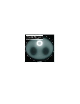
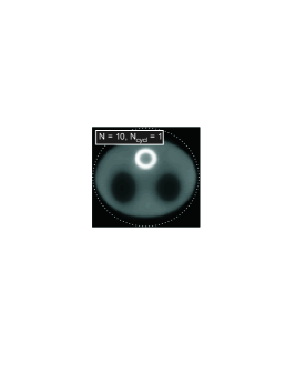
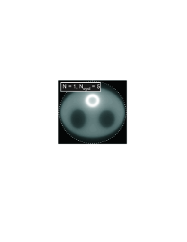
The iterations of the OS-EM method applied to exact data with $N_{t}=N_{r}=100$ and different values of $N$ are depicted in Figure 2. It can be seen that the 5-th iterate with EM has similar quality as the 1-th iterate with OS-EM for $N=5$. As a rough rule one can say that making $N$ cycles with the EM algorithm leads to an improvement similar to $1$ cycle with the OS-EM algorithm. This can also be recognized in the left image in Figure 3, where the evolution of the error is depicted with respect to the KL-distance.

In order to investigate the dependence of the OS-EM iteration on the discretization level, we repeated the experiment with $N_{t}=N_{r}=200$. The right image in Figure 3 shows the corresponding logarithmic error. As expected, the error is relatively independent on the discretization.

In the case of noisy data we apply the loping OS-EM iteration (5.5). The noisy data ${\boldsymbol{y}}_{j}^{\delta}$ is created by adding $5\%$ Poisson distributed noise to the simulated data ${\boldsymbol{y}}_{j}$, such that $4\pi/(N_{r}N_{\varphi})\sum\bigl{|}{\boldsymbol{y}}_{j}[i_{\varphi},i_{r}]-{\boldsymbol{y}}_{j}^{\delta}[i_{\varphi},i_{r}]\bigr{|}\cong 0.05$.

Remark 5.4

Our numerical experiments show that, for large $\delta$ and $\tau\cong 1$, far too many iterations are loped. A significant improvement can be obtained if $\tau=\tau(\delta)$ is chosen in dependence of the noise level, with $\tau(\delta)<1$ for large $\delta$ and $\tau(\delta)$ converging to some $\tau_{\infty}>1$ for $\delta\to 0$. It is clear that the asymptotic convergence analysis (for $\delta\to 0$) remains valid in such a situation.

Figure 4: Noisy data experiment: Iterates without loping (top line) and with loping (bottom line). The loping iterations are stopped automatically whereas their non-loping counterparts are stopped at the iteration cycle where $d(x^{*},x_{k}^{\delta})$ is minimal (which is not available in practice).

Figure 5: Noisy data experiment: Evolution of the relative error $\log\boldsymbol{d}({\boldsymbol{x}}^{*},{\boldsymbol{x}}_{k}^{\delta})$ for loping and non-loping OS-EM iterations.

Figure 6: Noisy data experiment: The $x$-axis shows the number of cycles, while the number of actually performed iterations within each cycle is shown at the $y$-axis.

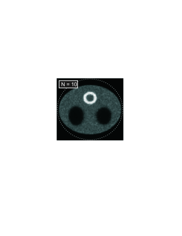
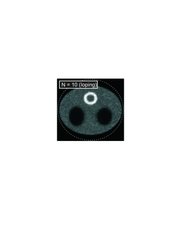
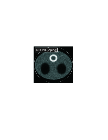
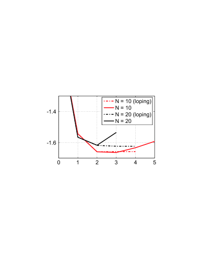
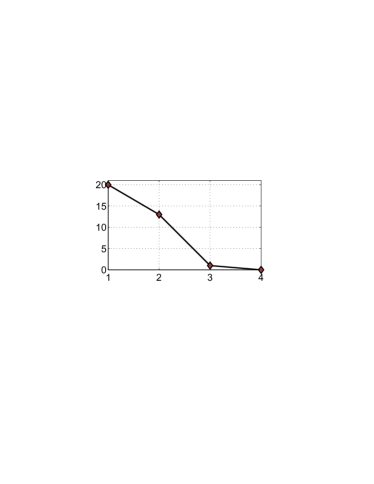
The reconstruction for noisy data with $N_{t}=N_{r}=100$ are depicted in Figure 4. For comparison purposes, results of the OS-EM iteration (without loping strategy) are also included. The loping OS-EM is automatically stopped according to (4.9) whereas their non-loping counterparts are stopped after the cycle with minimal error $\boldsymbol{d}({\boldsymbol{x}}^{*},{\boldsymbol{x}}_{k}^{\delta})$, which is not available in practice. All reconstructions are quite comparable. Figure 5 shows the evolution of the error with respect to the KL-distance. In this figure one also notices the semi-convergence of the non-loping iterations, which happens typically when applying non-regularized iterative schemes to ill-posed problems [2, 7, 10].

	$N$	$N_{\rm cycl}$	time (sec)	$\boldsymbol{d}({\boldsymbol{x}}^{*},{\boldsymbol{x}}_{k}^{\delta})$
loping OS-EM	10	4	13.4	0.022
OS-EM	10	3	9.2	0.022
loping OS-EM	20	4	13.4	0.024
OS-EM	20	2	6.3	0.024

Table 1: Comparison of the performance of different iterative methods. The non-loping iterations are stopped after the cycle with minimal error, whereas the loping OS-EM are automatically stopped according to (4.9).

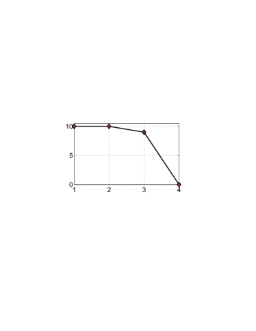
An inspection of Figure 5 shows that the regularized solution of the loping OS-EM methods (automatically stopped) have errors comparable to the optimal solution of their non-loping counterparts when stopped after the cycle with minimal error (which is not available in the practice). Figure 6 shows the number of actually performed iterations. Table 1 summarizes run times and errors with $N_{t}=N_{r}=100$, $N_{\rm angle}=100$ (with non-optimized Matlab implementation on HP Notebook with 2 GHz Intel Core Duo processor).

6 Conclusions

This article is devoted to the investigation of OS-EM type algorithms for solving systems of linear ill-posed equations. We focus on showing regularization properties of the proposed methods.

In the case of exact data, our approach originates an algorithm analog to the OS-EM iteration. We are able to prove monotonicity results with respect to the Kullback-Leibler distance as well as weak convergence in case of boundedness of the iterations. In the noisy data case, we propose a loping OS-EM iteration which differs from the OS-EM method due to the introduction of a loping strategy. This loping strategy renders the proposed iteration a regularization method. We prove monotonicity of the iterates and study stability properties of our method.

What concerns numerical effort, we conjecture that the loping OS-EM algorithm is at least as efficient as the well established OS-EM method. The numerical experiments with (5.5) for inverting the circular Radon transform support this conjecture. In the case of exact data, (5.5) reduces to a discretized version of the continuous OS-EM iteration applied to the system (5.3). However it is slightly different to the discrete OS-EM iteration of [8] since $\operatorname{\mathbf{B}}_{j}$ is not the exact transpose of $\operatorname{\mathbf{M}}_{j}$. Moreover, opposed to [8] our continuous convergence analysis applies independent on the discretization level.

References

- [1] A. De Cesaro, M. Haltmeier, A. Leitao, and O. Scherzer. On Steepest-Descent-Kaczmarz methods for regularizing systems of nonlinear ill-posed equations. Appl. Math. Comput., 202:596–607, 2008.
- [2] P. Deuflhard, H. W. Engl, and O. Scherzer. A convergence analysis of iterative methods for the solution of nonlinear ill–posed problems under affinely invariant conditions. Inverse Probl., 14:1081–1106, 1998.
- [3] P. P. B. Eggermont and V. N. LaRiccia. Maximum penalized likelihood estimation and smoothed EM algorithms for positive integral equations of the first kind. Numer. Funct. Anal. Optim., 17(7-8):737–754, 1996.
- [\hrefhttp://www.ams.org/mathscinet-getitem?mr=14086804] H. W. Engl, M. Hanke, and A. Neubauer. Regularization of inverse problems, volume 375 of Mathematics and its Applications. Kluwer Academic Publishers Group, Dordrecht, 1996.
- [5] M. Haltmeier, R. Kowar, A. Leitao, and O. Scherzer. Kaczmarz methods for regularizing nonlinear ill-posed equations II: Applications. Inverse Probl. Imaging, 1:507–523, 2007.
- [6] M. Haltmeier, A. Leitao, and O. Scherzer. Kaczmarz methods for regularizing nonlinear ill-posed equations I: convergence analysis. Inverse Probl. Imaging, 1:289–298, 2007.
- [7] M. Hanke, A. Neubauer, and O. Scherzer. A convergence analysis of Landweber iteration for nonlinear ill-posed problems. Numer. Math., 72:21–37, 1995.
- [8] H. M. Hudson and R. S. Larkin. Accelerated image reconstruction using ordered subsets projection data. IEEE Trans. Med. Imag., 13:601–609, 1994.
- [9] Alfredo N. Iusem. A short convergence proof of the EM algorithm for a specific Poisson model. Rebrape, 6(1):57–67, 1992.
- [10] B. Kaltenbacher, A. Neubauer, and O. Scherzer. Iterative Regularization Methods for Nonlinear Ill–Posed Problems, volume 6 of Radon Series on Computational and Applied Mathematics. de Gruyter, Berlin, 2008.
- [11] R. Kowar and O. Scherzer. Convergence analysis of a Landweber-Kaczmarz method for solving nonlinear ill-posed problems. Ill posed and inverse problems (book series), 23:69–90, 2002.
- [12] P. Kuchment and L. A. Kunyansky. Mathematics of thermoacoustic and photoacoustic tomography. European J. Appl. Math., 19:191–224, 2008.
- [13] H. N. Mülthei and B. Schorr. On an iterative method for a class of integral equations of the first kind. Math. Methods Appl. Sci., 9(2):137–168, 1987.
- [14] H. N. Mülthei and B. Schorr. On properties of the iterative maximum likelihood reconstruction method. Math. Methods Appl. Sci., 11(3):331–342, 1989.
- [15] G. Paltauf, R. Nuster, M. Haltmeier, and P. Burgholzer. Experimental evaluation of reconstruction algorithms for limited view photoacoustic tomography with line detectors. Inverse Probl., 23(6):81–94, 2007.
- [16] R. A. Redner and H. F. Walker. Mixture densities, maximum likelihood and the EM algorithm. SIAM Rev., 26(2):195–239, 1984.
- [17] E. Resmerita and R. S. Anderssen. Joint additive Kullback–Leibler residual minimization and regularization for linear inverse problems. Math. Methods Appl. Sci., 30(13):1527–1544, 2007.
- [18] E. Resmerita, H. W. Engl, and A. N. Iusem. The expectation-maximization algorithm for ill-posed integral equations: a convergence analysis. Inverse Problems, 23(6):2575–2588, 2007.
- [19] W. H. Richardson. Bayesian-based iterative method of image restoration. J. Opt. Soc. Am., 62:55–59, 1972.
- [20] O. Scherzer, M. Grasmair, H. Grossauer, M. Haltmeier, and F. Lenzen. Variational Methods in Imaging, volume 167 of Applied Mathematical Sciences. Springer, New York, 2008.
- [21] Y. Vardi, L. A. Shepp, and L. Kaufman. A statistical model for positron emission tomography. J. Amer. Statist. Assoc., 80(389):8–37, 1985. With discussion.
- [22] M. Xu and L. V. Wang. Photoacoustic imaging in biomedicine. Rev. Sci. Instruments, 77(4):041101, 2006.