Are low-degree p mode frequencies predictable from one cycle to the next?

Abstract

The Birmingham Solar-Oscillations Network (BiSON) has been collecting data for over $30\,\rm yrs$ and so observations span nearly three $11\,\rm yr$ solar activity cycles. This allows us to address important questions concerning the solar cycle and its effect on solar oscillations, such as: how consistent is the acoustic behaviour from one cycle to the next? We have used the p-mode frequencies observed in BiSON data from one solar activity cycle (cycle 22) to predict the mode frequencies that were observed in the next activity cycle (cycle 23). Some bias in the predicted frequencies was observed when short $108\,\rm d$ time series were used to make the predictions. We also found that the accuracy of the predictions was dependent on which activity proxy was used to make the predictions and on the length of the relevant time series.

¹School of Physics and Astronomy, University of Birmingham, Edgbaston, Birmingham B15 2TT
²Faculty of Arts, Computing, Engineering and Sciences, Sheffield Hallam University, Sheffield S1 1WB
³Astronomy Unit, School of Mathematical Sciences, Queen Mary, University of London, Mile End Road, London E1 4NS

1. Introduction

The frequencies of solar oscillations vary with solar activity (Woodard & Noyes 1985) and the changes in frequency can, in principle, be used to infer solar-cycle related structural changes in the Sun. Methods have been developed to remove solar cycle frequency shifts (e.g. Chaplin et al. 2004) to allow comparisons between the mode frequencies obtained from non-contemporaneous data and to enable accurate activity-independent structural inversions to be performed.

The Birmingham Solar-Oscillations Network (BiSON) has been recording data for over $30\,\rm yrs$, and so observations span nearly three solar cycles. We aim to take advantage of this to answer the following question: can the mode frequencies observed in cycle 22 be used to predict the mode frequencies observed in cycle 23? In other words, is it possible to produce a model that can be used to predict the mode frequencies observed in cycle 23?

Each $11\,\rm yr$ solar cycle is different from the previous one, for example, cycle 23 has been described as magnetically simpler than recent previous cycles (de Toma et al. 2004). Several different activity proxies can be used to measure the level of solar activity and, as each proxy responds to different physical processes, the amplitude and shape of each activity cycle depends upon which activity proxy is considered. With this in mind we aim to determine whether the acoustic behaviour of the Sun is predictable from one cycle to the next.

We begin this paper by describing how we used the mode frequencies, observed in cycle 22, to predict the mode frequencies observed in cycle 23 (Section 2). Then, in Section 3, we compare these predicted frequencies with the actual frequencies observed in cycle 23. Section 4 comprises a discussion of the results.

2. Predicting frequency shifts

An $11\,\rm yr$ BiSON time series is available, which covers the whole of cycle 22. To allow solar cycle frequency shifts to be examined this data set was split into contiguous $108\,\rm d$ time series. A standard likelihood maximization method was used to fit the power spectra of these time series (e.g. Chaplin et al. 1999), enabling the observed mode frequencies to be determined. The weighted mean activity level, $a$, observed during each $108\,\rm d$ time period was also calculated for four activity proxies, namely the $10.7\,\rm cm$ flux $(\rm F_{10.7})$, the HeI equivalent width (HeI EW), the Kitt Peak Magnetic Index (KPMI) and the International Sunspot Number (ISN).

A minimum activity reference set was determined by averaging the frequencies from five $108\,\rm d$ time series that were observed during the minimum activity epoch at the boundary between cycle 22 and cycle 23. We define the solar cycle frequency shifts as the difference between the frequencies given in the minimum activity reference set and the frequencies of the corresponding modes observed at different epochs and, consequently, different levels of activity. The size of a frequency shift has a well-known dependency on frequency and mode inertia and these dependencies were removed in the manner described in Chaplin et al. (2004). We have, therefore, determined the mean frequency shift at a given activity level. We now describe how these shifts were used to predict the mode frequencies observed in cycle 23.

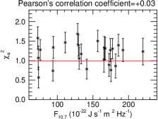
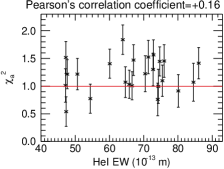
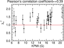
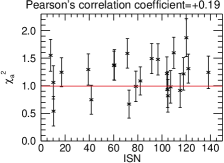
Figure 1.: The $\chi_{a}^{2}$ observed at different activity levels when four different activity proxies were used to predict the frequency shifts.

For low-degree p modes, the relationship between activity and mean frequency shift is approximately linear. A linear least squares fit was performed to determine the coefficients of the relationship between the mean frequency shifts observed during cycle 22 and the corresponding mean activity observed by each of the four activity proxies. These linear relationships were then used to predict the size of the mean frequency shift at a given activity level, which corresponds to a particular time period from cycle 23.

Let $\delta\nu_{1}(a)$ be the mean frequency shift predicted by the linear relationship for a given activity level, $a$. To determine the frequency shift for a particular mode, $\delta\nu_{n,l}(a)$, with degree, $l$, and radial order, $n$, it was necessary to scale $\delta\nu_{1}(a)$ with mode frequency and inertia. This was done using equation 4 of Chaplin et al. (2004). The resulting frequency shift, $\delta\nu_{n,l}(a)$, was added to the corresponding mode frequency stored in the minimum activity reference set to give a predicted frequency, and its associated errors, for a given epoch. The predicted frequencies were compared to the frequencies observed in BiSON data during the same time span and we now go on to describe the results of this comparison.

Table 1.: The weighted mean $\chi_{a}^{2}$ for the different activity proxies

Proxy	Weighted mean $\chi_{a}^{2}$	Distance from $\chi^{2}=1$
$\rm F_{10.7}$	$1.18\pm 0.06$	$3.1\sigma$
HeI EW	$1.20\pm 0.06$	$3.5\sigma$
KPMI	$1.30\pm 0.06$	$5.2\sigma$
ISN	$1.18\pm 0.06$	$3.1\sigma$

3. Analysis of results

To determine how accurate the prediction method is we have compared the predicted frequency of a mode at an activity level, $a$, with the frequency observed in BiSON data at the same activity level. The observed frequencies were determined by fitting the power spectrum of the corresponding $108\,\rm d$ time series using the standard likelihood maximization method (Chaplin et al. 1999).

The reduced $\chi^{2}$ between the predicted and the observed frequencies at a particular activity level was determined. Let $\chi_{a}^{2}$ be the reduced $\chi^{2}$ for all modes for which accurate fits to the data were obtained in a $108\,\rm d$ time series, observed during cycle 23. Errors on the reduced $\chi^{2}$ were taken to be $\sqrt{2/(N-1)}$, where $N$ is the number of data points used to calculate the reduced $\chi^{2}$. Figure 1 shows the variation of $\chi_{a}^{2}$ with activity, where each panel shows the results predicted by a different activity proxy. The vast majority of the observed $\chi_{a}^{2}$ are within $3\sigma$ of unity, which is the expected value if the model is accurate. However, for all activity proxies, the observed $\chi_{a}^{2}$ are predominately greater than unity, which implies there is some bias in the predicted results.

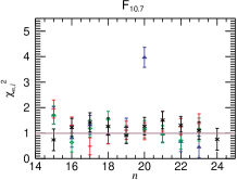
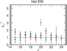
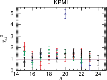
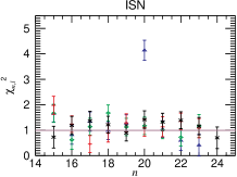
Figure 2.: The $\chi_{n,l}^{2}$ observed at different radial orders, $n$, when four different activity proxies were used to predict the frequencies.

To determine whether there is any correlation between the level of activity and the accuracy of the predicted frequencies the Pearson’s correlation coefficient between activity level and $\chi_{a}^{2}$ was calculated (see the values above the panels in Figure 1). None of the correlation coefficients are significant at a 95% confidence level. However, the correlation coefficient for the $10.7\,\rm cm$ flux result is smaller than for the other activity proxies. The results imply that the accuracy of the predictions made using the HeI EW, the ISN and the KPMI are marginally dependent on activity. We propose that this is true for the following reason. The HeI EW is mainly sensitive to the weak magnetic field and the ISN and KPMI are most sensitive to the strong magnetic field, while the $10.7\,\rm cm$ flux shows good sensitivity to both the strong and the weak magnetic flux. Therefore, we believe that to make accurate predictions at all activity levels it is necessary for the activity proxy to be responsive to both the strong and weak flux.

As a measure of the overall accuracy of the predictions the weighted mean $\chi_{a}^{2}$ was determined, and the results are shown in Table 1. All of the weighted mean $\chi_{a}^{2}$ are more than $3\sigma$ from unity, indicating there is some bias in the predicted frequencies. The weighted mean $\chi_{a}^{2}$ is noticeably larger for the KPMI than when the other proxies are used, which highlights the inadequacies of this proxy as a predictive tool.

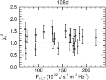
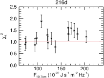
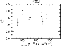
Figure 3.: The variation of $\chi_{a}^{2}$ with activity for time series of different lengths, when $108\,\rm d$ time series were used as the reference set.

We also investigated whether the accuracy of the predicted mode frequencies was dependent on frequency (or $n$). Let $\chi_{n,l}^{2}$ be the reduced $\chi^{2}$ for individual $n$ and $l$ across all activity levels. The results are shown in Figure 2. All of the proxies enable the frequencies to be predicted to a reasonable degree of accuracy as $\chi_{n,l}^{2}$ is within $3\sigma$ of unity for the vast majority of $n$ and $l$. Each panel of Figure 2 contains an outlier, which is observed because the frequency determined by the fitting procedure is inaccurate since at certain times this mode contains little power.

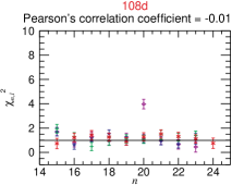
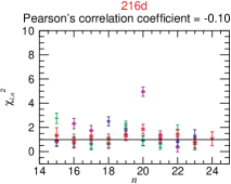
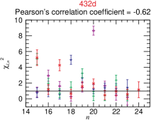
Figure 4.: The variation of $\chi_{n,l}^{2}$ with $n$ for time series of different lengths, when $108\,\rm d$ time series were used as the reference set.

Although not shown here, the Pearson’s correlation coefficients between $\chi_{n,l}^{2}$ and $n$ were found to be approximately zero implying the accuracy of the predictions is not dependent on $n$. However, it should be noted that this is only true for the range of $n$ examined here. Once we move outside this frequency range $(2200\,\rm\mu Hz\leq\nu\leq 3500\,\rm\mu Hz)$ the quality of both the fitted frequencies and the predictions deteriorates significantly.

3.1. Time series of different lengths

Next, we sought to determine whether the data observed in $108\,\rm d$ time series in cycle 22 could be used to predict the acoustic behaviour observed in longer ($216\,\rm d$, $432\,\rm d$) data sets from cycle 23. Figure 3 shows the variation of $\chi_{a}^{2}$ with activity when predictions were made for different length time series. The determined $\chi_{a}^{2}$ increases with the length of the time series, implying that the predictions for longer time series are less accurate. Additionally, the weighted mean $\chi_{a}^{2}$, which are quoted in Table 2 (when the $108\,\rm d$ time series are used to make the predictions), are found to be larger for the longer time series, indicating the $108\,\rm d$ time series can not be used to predict the frequencies observed in longer time series.

Figure 4 shows the variation of $\chi_{l,n}^{2}$ with radial order, $n$, for different length time series. The determined $\chi_{l,n}^{2}$ increase as $n$ decreases, especially in the longer time series, indicating that the predictions for low-$n$ modes are less accurate in long time series. Quoted above each panel in Figure 4 are the Pearson’s correlation coefficients, which become increasingly negative for the long time series and is in fact significant at a 95% confidence level for the $432\,\rm d$ time series. This is probably because it is more difficult to observe low-frequency modes in $108\,\rm d$ time series than in longer data sets and so the predicted frequencies are biased.

Finally we ask whether more accurate predictions are made if the frequencies observed in longer time series are used to define the relationship between frequency shift and activity. For example, we have used the mode frequencies observed in time series of length $216\,\rm d$ during cycle 22 to make predictions of the mode frequencies observed in $216\,\rm d$ time series in cycle 23. The observed weighted mean $\chi_{a}^{2}$, quoted in Table 2, indicate that the most accurate predictions are made when the time series used to make the predictions and the time series for which the predictions are required are both of the same length.

Table 2.: The weighted mean $\chi_{a}^{2}$ between the observed and predicted frequency shifts for different length time series.

Time series length	Weighted mean $\chi_{a}^{2}$	Distance from $\chi_{a}^{2}=1$
$108\,\rm d$ to predict $108\,\rm d$	$1.18\pm 0.06$	$3.1\sigma$
$108\,\rm d$ to predict $216\,\rm d$	$1.24\pm 0.07$	$3.5\sigma$
$216\,\rm d$ to predict $216\,\rm d$	$1.06\pm 0.07$	$0.9\sigma$
$108\,\rm d$ to predict $432\,\rm d$	$1.51\pm 0.10$	$5.3\sigma$
$216\,\rm d$ to predict $432\,\rm d$	$1.13\pm 0.10$	$1.4\sigma$
$432\,\rm d$ to predict $432\,\rm d$	$1.07\pm 0.10$	$0.8\sigma$

4. Discussion

We have shown that, when $108\,\rm d$ time series are used, there may be some evidence for a bias in the predictions, as the weighted mean $\chi_{a}^{2}$ are noticeably greater than unity, indicating that it may be problematic to use the $108\,\rm d$ time series to predict the mode frequencies. The accuracy of the predictions made using the $10.7\,\rm cm$ flux show least dependence on activity, probably because the $10.7\,\rm cm$ flux is sensitive to both the strong and the weak magnetic field. The predictions made using the KPMI were not as accurate as those made using the other models and so this proxy should not be used as a predictive tool.

The accuracy of the predictions decreases when $108\,\rm d$ time series are used to predict mode frequencies for longer time series and so $108\,\rm d$ time series can not be used to predict the acoustic behaviour observed in longer time series. The predicted frequencies were more accurate when longer data sets were used to make the predictions and when the time series from cycle 22, which were used to make the predictions, and the cycle 23 time series were of the same length. Note that this analysis has been performed using the mode frequencies observed in 2 solar cycles only but would ideally use the data from more solar cycles.

Acknowledgments.

We thank past and present members of the BiSON team and all those involved in the data collection process. The authors acknowledge the financial support of the Science and Technology Facilities Council (STFC).

References

- Chaplin et al. (1998) Chaplin W. J., Elsworth Y., Isaak G. R., Lines R., McLeod C. P., Miller B. A., New R., 1998, MNRAS, 300, 1077
- Chaplin et al. (1999) Chaplin W. J., Elsworth Y., Isaak G. R., Miller B. A., New R., 1999, MNRAS, 308, 424
- Chaplin et al. (2004) Chaplin W. J., Elsworth Y., Isaak G. R., Miller B. A., New R., 2004, MNRAS, 352, 1102
- de Toma et al. (2004) de Toma G., White O. R., Chapman G. A., Walton S. R., Preminger D. G., Cookson A. M., 2004, ApJ, 609, 1140
- Woodard & Noyes (1985) Woodard M. F., Noyes R. W., 1985, Nat, 318, 449