Flatband localization in the Anderson-Falicov-Kimball model

Abstract

The insulator-metal-insulator transition caused by a flatband is analyzed within dynamical mean-field theory using the Anderson-Falicov-Kimball model. We observe quantitative disagreement between the present approach and previous results. The presence of interactions enhances delocalization.

I Introduction

Recent studies have shown a new disorder-induced insulator-metal transition (MIT) of one-electron states, called the ”inverse Anderson transition”.inverse ; inverse2 The existence of this transition becomes already visible for non-interacting particles when the system has highly degenerated localized states forming a flatband. In a flatband localized states may melt into extended states due to disorder. For weak disorder, the localization is not a consequence of the strength of disorder but of the flatband. Increasing the degree of disorder localization-delocalization and delocalization-localization transitions appear.

New aspects must appear when we also consider interactions between particles of the system. The present work addresses this issue. The investigation of this problem is particularly rich. The interaction causes a Mott-Hubbard metal-insulator transition (MIT)Mott that competes with the Anderson transition.Anderson

The inverse Anderson transition has been studied using various numerical techniques, among them, level statistics,level $f(\alpha)$ characteristics of wave functionsfalfa and the participation radiusraio framework. However, these powerful tools are not adequate for interacting systems in which matrices of high order must be exactly diagonalized restricting the study to extremely small systems.

The dynamical mean-field theory (DMFT)pap4 is a good tool to investigate the Mott-Hubbard-Anderson MIT in lattice electrons with local interactions and disorder. The Anderson transition has for example been explored on the Bethe lattice considering the Hubbardpap1 and Falikov-Kimball models.Freer The metal and the insulator phases are detected by analyzing directly the local density of states (LDOS). The averaged LDOS can vanish in the band center at a critical disorder strength for a wide variety of averages.nos ; nos2 In particular, the arithmetic mean of this random one-particle quantity is non-critical at the Anderson transition and hence cannot help to detect the localization transition. By contrast, the geometric mean gives a better estimate of the averaged value of the LDOS,pap1 ; pap2 as it vanishes at a critical disorder strength and hence provides an explicit criterion for the Anderson localization.Mon2 ; pap3 ; pap4 We have adopted the Hölder mean and analyzed how the averaged LDOS depends on the Hölder parameter.

In this paper, we investigate the disorder-induced insulator-metal transition in a flatband of the Falikov-Kimball model using the DMFT. We present the ground-state phase diagram for different values of a parameter measuring the disorder strength and the dependence of the MIT transition on the Coulomb repulsion between fermions. Recently, we have applied the DMFT to this model. First, we showed that not only the geometric mean can offer a good approximation for the averaged LDOS providing an explicit criterion for Anderson localization. We found that the averaged LDOS can vanish in the band center at a critical disorder strength for a wide variety of generalized Hölder mean.nos Second, we have analyzed how the presence of the next-nearest-neighbor hopping influences the phase diagram of the ground state of this model, and, third, we studied the main effects of the long-range correlated disorder.nos2

This paper is organized as follows. In the next section II we introduce the Anderson-Falikov-Kimball model. The DMFT approach is described in section III. In section IV we present the results concerning the phase diagram. Finally in section V we conclude.

II Model

The Anderson-Falicov-Kimball modelpap2 is a tight binding model having two species of fermionic particles, mobile and immobile, which interact with each other when both are on the same lattice site. We introduce a local random potential for the mobile particles, giving rise to a competition between interaction and disorder. This model has been applied to mixed valence compounds of rare earth, transition metal oxides, binary alloys and metal ammonia solutions.Leu-Csa Its Hamiltonian is

$$H=\sum_{i}\epsilon_{i}c_{i}^{+}c_{i}-t\sum_{(ij)}c_{i}^{+}c_{j}+U\sum_{i}f_{i}^{+}f_{i}c_{i}^{+}c_{i},$$ (1)

where $c_{i}^{+}$ ($c_{i}$) and $f_{i}^{+}$ ($f_{i}$) are, respectively, the creation (annihilation) operators for the mobile and immobile fermions at lattice site $i$. $\epsilon_{i}$ is a random potential describing the local disorder, $t$ is the electron transfer integral connecting nearest-neighbor sites, and $U$ is the Coulomb repulsion when mobile and immobile particles occupy the same site. We consider that the occupation of immobile particles is site independent having a probability $p=1/2$. The number of mobile particles on site $i$ is given by $n_{i}=c_{i}^{+}c_{i}$. A chemical potential $\mu$ is introduced for the mobile subsystem to fix the system in the half-filled band ($\overline{n_{i}}=1/2$). Here, the energy will be given in units of the hopping element $t$ (i.e., $t=1$).

III Dynamical Mean-Field Equations

The DMFT is calculated from the Hilbert transform

$$G(E)=\int\frac{d\omega N_{0}(\omega)}{\eta(E)-\omega+1/G(E)}\;,$$ (2)

where $N_{0}(\epsilon)$ is the non-interacting density of states, $G(E)$ the translationally invariant Green function, and $\eta(E)$ a hybridization function describing the coupling of a selected lattice site with the rest of the system.pap3 For the flatband the non-interacting density of states is

$$N_{0}(E)=\frac{1}{2}[\delta(E-E_{0})+\delta(E+E_{0})]\;,$$ (3)

where the highly degenerated energies are $\pm E_{0}$. The relation between $G(E)$ and $\eta(E)$ is obtained in a straightforward way from Eq. (2) and Eq. (3)

$$\eta(E)=\sqrt{\frac{1}{4G(E)^{2}}+E_{0}^{2}}-\frac{1}{2G(E)}\;.$$ (4)

The LDOS is given bypap2

$$P(E,\epsilon_{i})=-\frac{1}{\pi}~{}Im~{}G(E,\epsilon_{i})\;,$$ (5)

where $G(E,\epsilon_{i})$ is the local $\epsilon_{i}$-dependent Green function. For the Anderson-Falicov-Kimball model we obtain thatnos

$$P(E,\epsilon_{i})=-\frac{s}{\pi}\frac{\alpha_{i}^{2}+s^{2}+(U/2)^{2}}{[\alpha_{i}^{2}+s^{2}+(U/2)^{2}]^{2}-U^{2}\alpha_{i}^{2}}\;,$$ (6)

where $\alpha_{i}=E-\epsilon_{i}-r$ and $r$ and $s$ are, respectively, the real and imaginary parts of $\eta(E)$.

We consider that $\epsilon_{i}$ is an independent random variable characterized by a probability function $p(\epsilon_{i})=\Phi(\Delta/2-|\epsilon_{i}|)/\Delta$, with $\Phi$ being the step function. The parameter $\Delta$ is a measure for the disorder strength. The self-consistent DMFT equations are closed inserting

$$G(E)=\int d\omega^{\prime}\frac{P_{q}(\omega^{\prime})}{E-\omega^{\prime}},$$ (7)

where

$$P_{q}(E)=\left\{\sum_{i}[P(E,\epsilon_{i})]^{q}\right\}^{1/q}\;.$$ (8)

The parameter $q$ defines the $q$-Hölder average. The arithmetic and geometric mean are found, respectively, using $q=1$ and $q\to 0$.

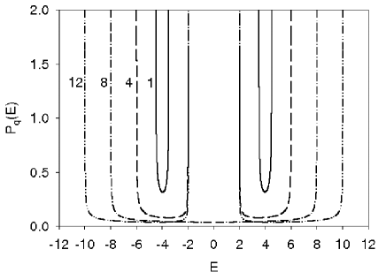
Figure 1: Density of states for disorder strength $\Delta=0$ and $U=1$, $4$, $8$ and $12$.

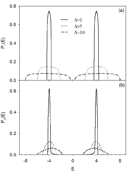
Figure 2: Averaged local density of states at $U=0$ and disorder strength $\Delta=1$, $5$, and $10$ for (a) $q=1$ and (b) $q=0$.

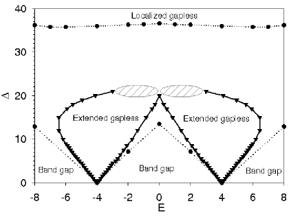
Figure 3: Ground-state phase diagram as a function of energy for $U=0$. The circles were taken from Ref. [1]. The triangles are determined from the numerical solution of the DMFT equations for $q=0$. The dashed region is the energy area in which we cannot estimate the transition points accurately. Lines are guides to the eye.

IV Results

First, we investigate the case without disorder. In this limit, where $\Delta=0$, we find, independently of $q$, that the analytical expression for the density of states of the flatband is

$$P_{q}(E)=\frac{E}{\pi\sqrt{[E^{2}-(E_{0}+U/2)^{2}][(E_{0}-U/2)^{2}-E^{2}]}},$$ (9)

if $|(E_{0}-U/2)|<|E|<|(E_{0}+U/2)|$ and $P_{q}(E)=0$, otherwise. Typical results are shown in Fig. 1. In order to compare our results with Refs. [1] and [2], we have set the highly degenerated state at $E_{0}=4$. Below $U=8$ we have two bands of bandwidth $U$. For $U>8$ we have also two bands, but now the bandwidth is constant and equal to $8$. The bandgap is always $|8-U|$. This bandgap for $U\gg 1$ exhibits the Mott insulator relationship between the bandgap and the repulsive Coulomb potential (bandgap $\sim U$). Note that for $U=8$ the system presents only one band of bandwidth $8$, and only for this case $P_{q}(0)\neq 0$.

Next, let us explore the case $\Delta\neq 0$. Here, the results are obtained numerically. We considered as initial $P_{q}(E)$ a uniform distribution with bandwidth greater than the Lifshitz band edge. Then we determined $G(E)$ in order to obtain $\eta(E)$ and finally the new values of $P_{q}(E)$. This procedure is repeated until we find the stable configuration.

Fig. 2 shows the energy dependence of the averaged LDOS for $U=0$ and typical values of $\Delta$. Note that the inclusion of the disorder (i.e., $\Delta\neq 0$) suppresses the highly degenerated localized states. We obtain the Anderson localization for a fixed $q$ varying the disorder strength $\Delta$ for each value of $U$, and then determining the values of $\Delta$ when $P_{q}(E)=0$. For the highly degenerated energy state, the arithmetic mean($q=1$) of the LDOS does not vanish at a finite critical disorder strength. Hence, we consider it to be non-critical at the Anderson transition. Using the geometric average ($q=0$), the LDOS vanishes at the highly degenerated energy state for a finite value of $\Delta$. The detection of the Anderson localization is obtained using $q=0$.

Fig. 3 presents the phase diagram of the ground state for the Anderson-Falikov-Kimball model as a function of energy for $U=0$ using the geometrical average. Our results are represented by triangles. The results of Ref. [1] are marked by circles. As we use an iterative process, our $P_{q}(E)$ not always converges to a stable value for large $\Delta$. Within the dashed area of Fig. 3 we cannot estimate the transition points accurately. We can observe three phases: extended gapless, localized gapless and band gap.pap2

The DMFT gives different results from the ones obtained in Refs. [1] and [2]. The DMFT approach reduces the extended phase, increasing the critical disorder $\Delta_{c}$ for the localization-delocalization transition and decreasing the one for the delocalization-localization transition. The considerable quantitative disagreement between both approaches requires new investigations to better understand these differences.

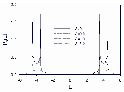
Figure 4: Averaged local density of states at $U=1$ and disorder strength $\Delta=0.1$, $0.5$, $1.0$ and $5.0$ for $q=0$.

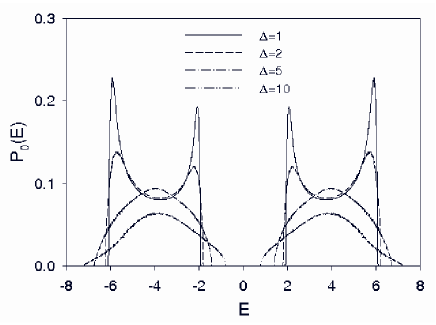
Figure 5: Averaged local density of states at $U=4$ and disorder strength $\Delta=1$, $2$, $5$ and $10$ for $q=0$.

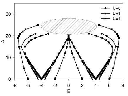
Figure 6: Ground-state phase diagram as function of energy for $U=0$, $1$ and $4$ obtained from the numerical solution of the DMFT equations. The dashed region is the energy area in which we cannot estimate the transition points accurately. Lines are guides to the eye.

We now consider the influence of the Coulomb repulsion $U$ on the results. Fig. 4 shows the averaged LDOS for $\Delta=0.1$, $0.5$, $1.0$ and $5.0$ at $U=1$. The results for $U=4$ are exhibited in Fig. 5, for $\Delta=1$, $2$, $5$ and $10$. As already observed for $U=0$, we find two symmetric bands. However, for small $\Delta$, the LDOS at the end bands, corresponding to the smallest and largest energies, are higher than those at the band centers. The band centers correspond to the highly degenerated states for $U=0$. Large $\Delta$ destroy the influence of the flatband and favour higher LDOS values at band centers and smaller ones at the edge bands. When $\Delta$ is large enough, the LDOS vanish and the extended phase disappears. For fixed $\Delta$, the bandwidth grows with increasing $U$.

Finally, in Figure 6 we present a complete ground-state phase diagram for three different values of $U$, namely $U=0$, $1$ and $4$. With $U$ increases the extended phase, showing that the interaction may enhance delocalization.

V Conclusions

In the present paper, we studied the solutions of the Anderson-Falicov-Kimball model involving a highly degenerated localized states forming a flatband. We have shown that the new disorder-induced insulator-metal transition of one-electron states, called ”inverse Anderson transition” can be obtained within dynamical mean field theory. However, we observed a considerable quantitative disagreement between the present approach and the previous results.inverse ; inverse2 The DMFT reduces the extended phase, increasing the critical disorder $\Delta_{c}$ for the localization-delocalization transition and decreasing $\Delta_{c}$ for the delocalization-localization transition.

We also studied the dependence of the MIT transition on the interaction between particles of the model and showed that increasing the interaction parameter reduces the extended phase for $U=0$.

As the doping of an impurity in the flatband has the same characteristics of the impurity states in the quantum Hall systeminverse2 , it would be interesting to do similar calculations for such a system.

VI Acknowledgments

Financial support of Conselho Nacional de Pesquisas Cientificas (CNPq) is acknowledged.

References

- (1) M. Goda, S. Nishino, and H. Matsuda, Phys. Rev. Lett. 96, 126401 (2006).
- (2) S. Nishino, and H. Matsuda, and M. Goda, J. Phys. Soc. Japan 76, 024709 (2007).
- (3) N. F. Mott, Proc. Phys. Soc. London, Sect. A 62, 416 (1949).
- (4) P. W. Anderson, Phys. Rev. 109, 1492 (1958).
- (5) E. Hofstetter and M. Schreiber, Phys. Rev. B 48, 16979 (1993).
- (6) A. Chhabra and R. V. Jensen, Phys. Rev. Lett. 62, 1327 (1989).
- (7) M. Schreiber, Phys. Rev. B 31, 6146 (1985).
- (8) V. Dobrosavljevic and G. Kotliar, Phys. Rev. Lett. 78, 3943 (1997).
- (9) K. Byczuk, W. Hofstetter and D. Vollhardt, Phys. Rev. Lett. 94, 056404 (2005).
- (10) J. K. Freericks and V. Zlatic, Rev. Mod. Phys. 75, 1333 (1993).
- (11) A. M. C. Souza, D. O. Maionchi, and H. J. Herrmann, Phys. Rev. B 76, 035111 (2007).
- (12) D. O. Maionchi, A. M. C. Souza, H. J. Herrmann, and R. N. da Costa Filho, Phys. Rev. B 77, 245126 (2008).
- (13) K. Byczuk, Phys. Rev. B 71, 205105 (2005).
- (14) M. Romeo, V. Da Costa and F. Bardou, Eur. Phys. J B 32, 513 (2003).
- (15) V. Dobrosavljevic, A. A. Pastor and B. K. Nikolic, Europhys. Lett. 62, 76 (2003).
- (16) K. Leung and F. S. Csajkall, J. Chem. Phys. 108, 9050 (1998).