Time-dependent angular analysis of the decays $B_{d}^{0}\to J/\psi K^{*0}$ and $B_{s}^{0}\to J/\psi\phi$

Abstract

In this paper we present the description of the flavor-untagged decays $B_{d}^{0}\to J/\psi K^{*0}$ and $B_{s}^{0}\to J/\psi\phi$ in the transversity basis. The study of these $B$ mesons in that basis makes it possible to extract information about flavor SU(3) symmetry and to verify if the factorization assumption is feasible for the decay $B_{d}^{0}\to J/\psi K^{*0}$. The lifetime ratio $\bar{\tau}_{s}/\tau_{d}$ is also extracted with this description.

I INTRODUCTION

Both decays considered in the present analysis, $B_{d}^{0}\to J/\psi K^{*0}$ and $B_{s}^{0}\to J/\psi\phi$, are decays of a pseudo-scalar to a vector-vector intermediate state. The observables of the angular distributions, the linear polarization amplitudes and the strong relative phases of the $B$ mesons that decay in such a way, can be extracted by their description in the transversity basis fleischer . By measuring those observables, we can obtain important information about flavor SU(3) symmetry and the factorization assumption related with these decays. The former requires that the linear polarization amplitudes and the strong relative phases characterizing these decays should have the same values fleischer ; gronau . Factorization states that, in the absence of final-state interactions (FSI), the strong phases are 0 (mod $\pi$) fleischer ; browder for the $B_{d}^{0}\to J/\psi K^{*0}$. In this paper we describe the flavor-untagged decays $B_{d}^{0}\to J/\psi K^{*0}$ and $B_{s}^{0}\to J/\psi\phi$ in the transversity basis. The final measurements of these analyses are reported in Ref. bd.bs.untagged .

II THE ANGULAR DESCRIPTION OF THE DECAYS $B_{d}^{0}\to J/\psi K^{*0}$ AND $B_{s}^{0}\to J/\psi\phi$

Due to the same 4-track topology, the decays under study can be described by the same transversity basis (see Fig. 1). We denote by $\boldmath{\omega}=\left\{\varphi,\cos\theta,\cos\psi\right\}$ the set of the angular variables for this basis.

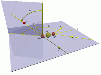
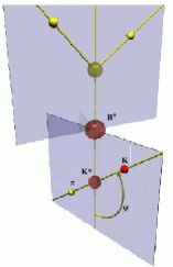
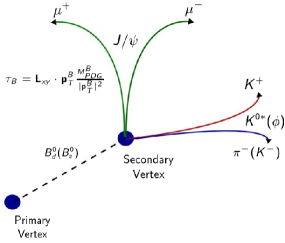
Figure 1: The angular variables of the transversity basis $\varphi$ and $\cos\theta$ are defined in the $J/\psi$ rest frame (left), and $\cos\theta$ in the $K^{*0}$ rest frame relative to the negative direction of the $J/\psi$ in that frame (center). The translation of this basis to the decay $B_{s}^{0}\to J/\psi\phi$ is straightforward due to the same 4-vertex track topology for the decays (right).

For the $B_{d}^{0}$ system, we take into account the interference between the $K\pi$ $P$- and $S$-wave amplitudes as described in Ref. babar . Therefore, the differential decay rate for the untagged decay $B_{d}^{0}\to J/\psi K^{*0}$ is given by fleischer ; babar :

$$\frac{d^{4}{\cal P}}{d\boldmath{\omega}\;dt} \propto e^{-t/\tau_{d}}\left\{\cos^{2}\lambda\left[|A_{0}|^{2}f_{1}(\boldmath{\omega})+|A_{\parallel}|^{2}f_{2}(\boldmath{\omega})+|A_{\perp}|^{2}f_{3}(\boldmath{\omega})-\zeta\;\mathrm{Im}(A_{\parallel}^{*}A_{\perp})f_{4}(\boldmath{\omega})+\mathrm{Re}(A_{0}^{*}A_{\parallel})f_{5}(\boldmath{\omega})\right.\right.$$

$$+ \left.\zeta\;\mathrm{Im}(A_{0}^{*}A_{\perp})f_{6}(\boldmath{\omega})\right]+\sin^{2}\lambda\cdot f_{7}(\boldmath{\omega})+\frac{1}{2}\sin 2\lambda\left[f_{8}(\boldmath{\omega})\cos\left(\delta_{2}-\delta_{1}-\delta_{s}\right)|A_{\parallel}|\right.$$

$$+ \left.f_{9}(\boldmath{\omega})\sin\left(\delta_{2}-\delta_{s}\right)|A_{\perp}|+\left.f_{10}(\boldmath{\omega})\cos\delta_{s}\cdot|A_{0}|\right]\right\},$$

where $\tau_{d}$ is the $B_{d}^{0}$ lifetime, $\zeta=+1(\zeta=-1)$ is for an initially produced $K^{+}(K^{-})$; $\lambda,\delta_{s}$, and $f_{i}(\boldmath{\omega})$ are defined in Refs. fleischer ; babar . If any of the strong phases, $\delta_{1}\equiv\arg[A_{\parallel}^{*}A_{\perp}]$ and $\delta_{2}\equiv\arg[A_{0}^{*}A_{\perp}]$, are not consistent with $0($mod$\thinspace\pi)$, then the factorization assumption is not valid for the decay $B_{d}^{0}\to J/\psi K^{*0}$.

In the $B_{s}^{0}$ system, since the standard model predicts a very small CP-violating phase lenz , we assume CP conservation for simplicity. From this, the differential decay rate for the untagged decay $B_{s}^{0}\to J/\psi\phi$ is given by fleischer :

$$d^{4}{\cal P}/\left(d\omega\;dt\right)\propto e^{-\Gamma_{L}t}\left[|A_{0}|^{2}f_{1}(\omega)+|A_{\parallel}|^{2}f_{2}(\omega)+\mathrm{Re}(A_{0}^{*}A_{\parallel})f_{5}(\omega)\right]+e^{-\Gamma_{H}t}|A_{\perp}|^{2}f_{3}(\omega),$$ (2)

where $\Gamma_{L(H)}\equiv 1/\tau_{L(H)}$ is the inverse of the lifetime corresponding to the light (heavy) mass eigenstate. For this decay, we have access to the same linear polarization amplitudes as for the $B_{d}^{0}$ and the phase $\delta_{\parallel}$, which is related with $\delta_{1}$ and $\delta_{2}$ by means of the relation $\delta_{\parallel}=\delta_{2}-\delta_{1}$. In this analysis, we also measure the mean lifetime $\bar{\tau}_{s}\equiv 1/\bar{\Gamma}=2/\left(\Gamma_{L}+\Gamma_{H}\right)$. If flavor SU(3) fleischer (or U(3) gronau ) symmetry is valid, then the linear amplitudes and the strong phases should be consistent with being equal for both the $B_{d}^{0}$ and $B_{s}^{0}$ mesons.

III THE MONTE CARLO REWEIGHTING

The distributions of certain kinematic variables in the Monte Carlo (MC) simulation, such as the transverse momentum $p_{T}$ of the particles, do not agree well with data. The D0 Detector run2det has a tracking and a muon systems such that the muon reconstruction is well understood. Because of this, we choose the $p_{T}(J/\psi)$ distribution to weight the generated MC distributions to agree with that of data. The comparison of some kinematic distributions before and after reweighting is shown in Fig. 2.

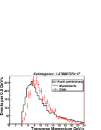
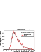
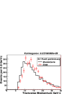
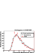
Figure 2: $p_{T}(J/\psi)$ (top) and $p_{T}(B_{d}^{0})$ (bottom) distributions before (left) and after (right) reweighting for the decay $B_{d}^{0}\to J/\psi K^{*0}$ using the histogram of the $p_{T}(J/\psi)$ distribution. The reweighting method improves the MC distributions, as can be seen from the Kolmogorov tests. Similar histograms are obtained for the decay $B_{s}^{0}\to J/\psi\phi$

IV THE ANGULAR EFFICIENCY $\epsilon({\boldmath\omega})$

We need to take into account the effect of the detector in the theoretical distributions Eqs. (II) and (2). We model this effect assuming that it can be written as a product of three polynomials $\epsilon(\omega)=p_{1}(\varphi)p_{2}(\cos\theta)p_{3}(\cos\psi)$. The coefficients of these polynomials are obtained by fitting the angular distributions of the reweighted MC. For the $B_{d}^{0}$ decays, the polynomials that give us the best modeling for $\epsilon(\omega)$ are those shown in Fig. 3. We follow the same procedure to obtain the polynomials for the decay $B_{s}^{0}\to J/\psi\phi$.

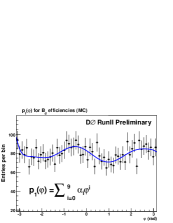
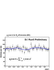
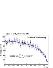
Figure 3: Polynomials $p_{i}$ for the $B_{d}^{0}$ angular efficiencies.

V THE ANGULAR PROBABILITY DISTRIBUTION FUNCTIONS

To extract the angular and lifetime parameters that describe the flavor-untagged decays $B_{d}^{0}\to J/\psi K^{*0}$ and $B_{s}^{0}\to J/\psi\phi$, we need to write the Eqs. (II) and (2) as probability distribution functions (pdf). The angular pdfs for the $j$-th $B_{d}^{0}$ and $B_{s}^{0}$ candidates are given by:

$$\mathcal{F}_{B_{d}^{0}}(|A_{0}|^{2},|A_{\parallel}|^{2},\delta_{1},\delta_{2},\tau_{d}) = \frac{\varepsilon(\omega_{j})}{N_{B_{d}^{0},sig}}\sum_{i=1}^{10}g_{i}f_{i}(\omega_{j}),$$ (3)

$$\mathcal{F}_{B_{s}^{0}}(|A_{0}|^{2},|A_{\parallel}|^{2},\delta_{\parallel},\bar{\tau}_{s}) = \frac{\epsilon_{s}(\omega_{j})}{N_{B_{s}^{0},sig}}\left[\mathcal{T}_{sig}^{L}\sum_{i=1,2,5}h_{i}f_{i}(\omega_{j})+\mathcal{T}_{sig}^{H}h_{3}f_{3}(\omega_{j})\right],$$ (4)

respectively, where $g_{i}(h_{i})$ are the coefficients of Eq.(II) [Eq.(2)] and $N_{B_{d(s)},sig}$ is the normalization factor. The complete description of the log-likehood functions for both decays is reported in Ref. bd.bs.untagged .

References

• (1) A.S.Β Dighe, I.Β Dunietz, and R.Β Fleischer, Eur. Phys. J. C6, 647 (1999).
• (2) M.Β Gronau and J.L.Β Rosner, arXiv:0808.3761 [hep-ex] (2008), submitted to Phys. Lett. B.
• (3) T.E.Β Browder, K.Β Honscheid, and D.Β Pedrini, Annu. Rev. Nucl. Part. Sci. 46, 395 (1996).
• (4) V.Β Abazov et al. [D0 Collaboration], arXiv:0810.0037 [hep-ex] (2008), submitted to Phys.Β Rev.Β Lett.
• (5) B. Aubert et al. [BaBar Collaboration], Phys. Rev. D 71, 032005 (2005).
• (6) A. Lenz and U. Nierste, JHEP 06, 072 (2007).
• (7) V. Abazov et al. [D0 Collaboration], Nucl. Instr. and Meth. Phys. Res. A 565, 463 (2006).