Hierarchical bag of paths for kernel based shape classification

Abstract

Graph kernels methods are based on an implicit embedding of graphs within a vector space of large dimension. This implicit embedding allows to apply to graphs methods which where until recently solely reserved to numerical data. Within the shape classification framework, graphs are often produced by a skeletonization step which is sensitive to noise. We propose in this paper to integrate the robustness to structural noise by using a kernel based on a bag of path where each path is associated to a hierarchy encoding successive simplifications of the path. Several experiments prove the robustness and the flexibility of our approach compared to alternative shape classification methods.

1 Introduction

The skeleton of a $2D$ shape is defined as the location of the singularities of the signed distance function to the border of the shape. This structure has several interesting properties: it is thin, homotopic to the shape, invariant under rigid transformations of the plane and most importantly it has a natural interpretation as a graph. The representation of a shape by a skeletal (or shock) graph has become popular owing the good properties of this representation inherited from the properties of the skeleton. However, beside all this good properties, the skeletonization is not continuous and small perturbations of the boundary insert structural noise within the graph encoding the shape.

Several graph based methods have been proposed to compute a distance between shapes robust to such a structural noise. Sharvit et al. [1] propose a graph matching method based on a graduated assignment algorithm. Siddiqi [2] proposes to transform the shock graph into a tree and then applies a tree matching algorithm. Pellilo [3] uses the same tree representation but transforms the tree matching problem into a maximal clique problem within a specific association graph.

All the above graph methods operate directly on the space of graphs which contains almost no mathematical structure. This lack of mathematical structure forbids the use of basic statistical tools such as the mean or the variance. Graph kernels provide an elegant solution to this problem. Using appropriate kernels, graphs can be mapped either explicitly or implicitly into a vector space whose dot product corresponds to the kernel function. All the “natural” operations on a set of graphs which were not defined in the original graph space are now possible into this transformed vector space. In particular, graph kernels may be combined with the kernelised version of robust classification algorithms such as the Support Vector Machine (SVM).

A Graph kernel used within the shape representation framework should take into account the structural noise induced by the skeletonization process. Bunke [4] proposes to combine edit distance and graph kernels by using a set of $n$ prototype graphs $\{g_{1},\dots,g_{n}\}$. Given a graph edit distance $d(.,.)$, Bunke associates to each graph $g$ the vector $\phi(g)=(d(g,g_{1})\dots,d(g,g_{n}))$. The kernel $k(g_{1},g_{2})$ between the two graphs $g_{1}$ and $g_{2}$ is then defined as the dot product $<\phi(g_{1}),\phi(g_{2})>$.

Neuhaus [5] proposes a similar idea by defining for a prototype graph $g_{0}$, the kernel: $k_{g_{0}}(g,g^{\prime})=\frac{1}{2}\left(d^{2}(g,g_{0})+d^{2}(g_{0},g^{\prime})-d^{2}(g,g^{\prime})\right)$, where $d(.,.)$ denotes the graph edit distance. Several graph prototypes may be incorporated by summing or multiplying such kernels. Using both Neuhaus [5] and Bunke [4] kernels two close graphs should have close edit distance to the different graph prototypes. The metric induced by such graph kernels is thus relative both to the weights used to define the edit distance and to the graph prototypes. This explicit use of prototype graphs may appear as artificial in some application. Moreover, the definite positive property of these kernels may not in general be guaranteed.

Suard [6] proposes to use the notion of bag of paths of finite length for shape matching. This method associates to each graph all its paths whose length is lower than a given threshold. The basic idea of this approach is that two close shapes should share a large amount of paths. A kernel between these sets should thus reflect this proximity. However, small perturbations may drastically reduce the number of common paths between two shapes (Section 3.2). Moreover, the straightforward definition of a kernel between set of paths does not lead to a definite positive kernel (Section 2.1).

This paper proposes a new definite positive kernel between set of paths which takes into account the structural noise induced by the skeletonization process. We first present in Section 2 the bag of paths approach for shape similarity. Our contributions to this field are then presented in Section 3. The effectiveness of our method is demonstrated through experiments in Section 4.

2 Kernels on bag of paths

Let us consider a graph $G=(V,E)$ where $V$ denotes the set of vertices and $E\subset V\times V$ the set of edges. As mentioned in Section 1 a bag of paths $P$ of length $s$ associated to $G$ contains all the paths of $G$ of length lower than $s$. We denote by $\left\lvert P\right\rvert$ the number of paths inside $P$. Let us denote by $K_{path}$ a generic kernel between paths. Given two graphs $G_{1}$ and $G_{2}$ and two paths $h_{1}\in P_{1}$ and $h_{2}\in P_{2}$ of respectively $G_{1}$ and $G_{2}$, $K_{path}(h_{1},h_{2})$ may be interpreted as a measure of similarity between $h_{1}$ and $h_{2}$ and thus as a local measure of similarity between these two graphs. The aim of a kernel between bags of paths consits to agregate all these local measures between pairs of paths into a global similarity measure between the two graphs.

2.1 The max kernel

This first method, proposed by Suard [6], uses the kernel $K_{path}$ as a measure of similarity and computes for each path $h_{1}\in P_{1}$ the similarity with its closest path in $P_{2}$($\max_{h_{j}\in P_{2}}~\mbox{$K_{path}$}(h_{1},h_{j})$). A first global measure of similarity between $P_{1}$ and $P_{2}$ is then defined as:

$$\hat{K}_{max}(G_{1},G_{2})=\hat{K}_{max}(P_{1},P_{2})=\frac{1}{\left\lvert P_{1}\right\rvert}\sum_{h_{i}\in P_{1}}\max_{h_{j}\in P_{2}}K_{path}(h_{i},h_{j}).$$ (1)

The function $\hat{K}_{max}(G_{1},G_{2})$ is however not symmetric according to $G_{1}$ and $G_{2}$. Suard obtains a symmetric function interpreted as a graph kernel by taking the mean of $\hat{K}_{max}(G_{1},G_{2})$ and $\hat{K}_{max}(G_{2},G_{1})$:

$$\mbox{$K_{max}$}(G_{1},G_{2})=\tfrac{1}{2}\left[\hat{K}_{max}(G_{1},G_{2})+\hat{K}_{max}(G_{2},G_{1})\right].$$ (2)

This kernel is not positive definite in general. However as shown by Haasdonk [7], SVM with indefinite kernels have in some cases a geometrical interpretation as the maximization of distances between convex hulls. Moreover, experiments (section 4, and [6]) show that this kernel usually leads to valuable results.

2.2 The matching kernel

The non definite positiveness of the kernel $K_{max}$ is mainly due to the max operator. Suard [6] proposes to replace the kernel $K_{path}$ by a kernel which decreases abruptly when the two paths are different. The resulting kernel is defined as:

$$\mbox{$K_{matching}$}(G_{1},G_{2}) = \mbox{$K_{matching}$}(P_{1},P_{2})=$$

$$\frac{1}{\left\lvert P_{1}\right\rvert}\frac{1}{\left\lvert P_{2}\right\rvert}\sum_{h_{i}\in P_{1}}\sum_{h_{j}\in P_{2}}\exp\left(\frac{-d^{2}_{path}(h_{i},h_{j})}{2\sigma^{2}}\right).$$

where $d_{path}$ is the distance associated to the kernel $K_{path}$ and defined by: $d_{path}^{2}(h_{1},h_{2})=K_{path}(h_{1},h_{1})+K_{path}(h_{2},h_{2})-2K_{path}(h_{1},h_{2})$.

The resulting function defines a definite positive kernel. This kernel relies on the assumption that using a small value of $\sigma$, the couple of paths with the smallest distance will predominate the others in equation 2.2. This kernel may thus lead to erroneous results if the distance are of the same order of magnitude than $\sigma$ or if several couples of paths have nearly similar distances.

2.3 The change detection kernel

Desobry [8] proposed a general approach for the comparison of two sets which has straightforward applications in the design of a kernel between bags (sets) of paths. Desobry models the two sets as the observation of two sets of random variables in a feature space and proposes to estimate a distance between the two distributions without explicitly building the pdf of the two sets.

The feature space considered by Desobry is based on the normalised kernel ($K(h,h^{\prime})=K_{path}(h,h^{\prime})/\sqrt{(K_{path}(h,h)K_{path}(h^{\prime},h^{\prime}))}$). Using such a kernel we have $\|h\|^{2}_{K}=K(h,h)=1$ for any path. The image in the feature space of our set of paths lies thus on an hypersphere of radius $1$ centered at the origin (Fig. 1). Desobry defines a region on this sphere by using a single class $\nu$-SVM. This region corresponds to the density support estimate of the unknown pdf of the set of paths [8].

Using Desobry’s method, two set of vectors are thus map onto two regions of the unit sphere and the distance between the two regions corresponds to a distance between the two sets. Several kernels based on this mapping have been proposed:

(a) Sets on the unit sphere

(b) original

(c) edge protrusion

(d) node insertion

Figure 1: Separating two sets using one-class SVM (a). The symbols $(w_{1},\rho_{1})$ and $(w_{2},\rho_{2})$ denote the parameters of the two hyperplanes which are represented by dashed lines. Influence of small perturbations on the bag of paths ((b), (c) and (d))

1. Desobry proposed [8] to define the distance between the two spherical arcs as a contrast measure defined by: $d_{Desobry}^{2}(P_{1},P_{2})=\frac{\arccos\left(\frac{w_{1}K_{1,2}w_{2}}{\left\|w_{1}\right\|\left\|w_{2}\right\|}\right)}{\arccos\left(\frac{\rho_{1}}{\left\|w_{1}\right\|}\right)+\arccos\left(\frac{\rho_{2}}{\left\|w_{2}\right\|}\right)}.$ This distance is connected to the Fisher ratio (see [8, Section IV]). However, the definite positiveness of the Gaussian RBF kernel based on this distance remains to be shown.

2. Suard [6] proposed the following kernel: $K_{Suard}(G_{1},G_{2})=K_{Suard}(P_{1},P_{2})=\rho_{1}\rho_{2}\sum_{h_{i}\in P_{1}}\sum_{h_{j}\in P_{2}}\alpha_{1,i}\ K_{path}(h_{i},h_{j})\alpha_{2,j}$ with $w_{1}=(\alpha_{1,1},\ldots,\alpha_{1,\left\lvert P_{1}\right\rvert})$ and $w_{2}=(\alpha_{2,1},\ldots,\alpha_{2,\left\lvert P_{2}\right\rvert})$.

   This kernel is definite positive, but does not correspond to any straightforward geometric interpretation.

2.4 Path kernel

All the kernels between bags of paths defined in Section 2 are based on a generic kernel $K_{path}$ between paths. A kernel between two paths $h_{1}=(v_{1},\dots,v_{n})$ and $h^{\prime}=(v^{\prime}_{1},\dots,v^{\prime}_{p})$ is classically [9] built by considering each path as a sequence of nodes and a sequence of edges. This kernel denoted $K_{classic}$ is then defined as $0$ if both paths have not the same size and as follows otherwise:

$$\begin{split}K_{classic}(h,h^{\prime})=K_{v}(\varphi(v_{1}),\varphi(v^{\prime}_{1}))\overset{\left\lvert h\right\rvert}{\underset{i=2}{\prod}}K_{e}(\psi(e_{v_{i-1}v_{i}}),\psi(e_{v^{\prime}_{i-1}v^{\prime}_{i}}))K_{v}(\varphi(v_{i}),\varphi(v^{\prime}_{i}))\end{split}$$ (4)

where $\varphi(v)$ and $\psi(e)$ denote respectively the vectors of features associated to the node $v$ and the edge $e$. The terms $K_{v}$ and $K_{e}$ denote two kernels between respectively nodes and edge’s features. For the sake of simplicity, we have used Gaussian RBF kernels between the attributes of nodes and edges (Section 4).

3 Hierarchical kernels

Since the main focus of this paper is a new kernel method for shape classification, the construction of skeletal graphs from shapes has been adressed using classical methods. We first build a skeleton using the method proposed by Siddiqi [2]. However the graph we build from the skeleton does not correspond to the shock graph proposed by Siddiqi. Indeed, this graph provides a precise description of the shape but remains sensitive to small perturbations of the boundary. We rather use the construction scheme proposed by Suard [6] and Ruberto [10] which consists to select as node all the pixels of the skeleton which correspond to end points or junctions. These nodes are then connected by edges, each edge being associated to one branch of the skeleton. Given a skeletal graph $G$ we valuate each of its edge by an additive weight measure and we consider the maximal spanning tree $T$ of $G$. The bag of path associated to $G$ is built on the tree $T$. Note that, the skeletonization being homotopic we have $G=T$ if the $2D$ shape does not contain any hole.

3.1 Bag of path kernel

None of the bag of path kernels proposed by Desobry or Suard (Section 2) is both definite positive and provides a clear geometrical interpretation. We thus propose a new kernel based on the following distance:

$$d_{change}^{2}(P_{1},P_{2})=\arccos\left(\frac{w_{1}K_{1,2}w_{2}}{\left\|w_{1}\right\|\left\|w_{2}\right\|}\right).$$ (5)

This distance corresponds to the angle $\alpha$ between the two mean vectors $w_{1}$ and $w_{2}$ of each region (Fig. 1). Such an angle may be interpreted as the geodesic distance between two points on the sphere and has thus a clear geometrical interpretation. Based on this distance we use the Gaussian RBF kernel:

$$K_{change}(G_{1},G_{2})=K_{change}(P_{1},P_{2})=\exp\left(\frac{-d^{2}_{change}(P_{1},P_{2})}{2\sigma^{2}}\right).$$ (6)

This kernel is definite positive since the normalized scalar product is positive definite and $\arccos$ is bijective on $[0,1]$. The Gaussian RBF kernel based on this distance is thus definite positive (see [11] for further details).

3.2 Hierarchical kernel between paths

A mentioned in Section 1, the use of kernels between bags of paths within the shape matching framework relies on the assumption that the graphs associated to two similar shapes share a large amount of similar paths. This assumption is partially false since a small amount of structural noise may have important consequences on the set of paths. Let us for example, consider the small deformation of the square (Fig. 1(b)) represented on Fig. 1(c). This small deformation transforms the central node in Fig. 1(b) into an edge (Fig. 1(c)). Consequently graphs associated to these two shapes only share two paths of length $2$ (the ones which connect the two corners on the left and right sides). In the same way, a small perturbation of the boundary of the shape may add branches to the skeleton(Fig. 1(d)). Such additional branches i) split existing edges into two sub edges by adding a node and ii) increase the size of the bag of path either by adding new paths or by adding edges within existing paths.

The influence of small perturbations of the shape onto an existing set of paths may thus be modeled by node and edge insertions along these paths. In order to get a path kernel robust against structural noise we associate to each path a sequence of successively reduced paths, thus forming a hierarchy of paths. Our implicit assumption is that, if a path has been elongated by structural noise one of its reduced version should corresponds to the original path.

The reduction of a path is performed either by node removal or edge contraction along the path. Such a set of reduction operations is compatible with the taxinomy of topological transition of the skeleton compiled by Giblin and Kimia [12]. Note that, since all vertices have a degree lower than $2$ along the path these operations are well defined. In order to select both the type of operation and the node or the edge to respectively remove or contract we have to associate a weight to each node and edge which reflects its importance according to the considered path and the whole graph.

Let us consider a skeletal graph $G$, its associated maximal spanning tree $T$ and a path $h=(v_{1},\dots,v_{n})$ within $T$. We valuate each operation on $h$ as follows:

Node removal :

Let us denote by $v_{i}$, $i\in\{2,\dots,n-1\}$ the removed node of the path $h$. The node $v_{i}$ has a degree greater than $2$ in $T$ by construction. Our basic idea consists to valuate the importance of $v_{i}$ by the total weight of the additional branches which justify its existence within the path $h$. For each neighbor $v$ of $v_{i}$ not equal to $v_{i-1}$ nor $v_{i+1}$ we compute the weight $W(v)$ defined as the addition of the weight of the tree rooted on $v$ in $T-\{e_{v_{i}v}\}$ and the weight of $e_{v_{i}v}$. This tree is unique since $T$ is a tree. The weight of the node $v_{i}$ (and the cost of its removal) is then defined as the sum of weight $W(v)$ for all neighbors $v$ of $v_{i}$ (excluding $v_{i-1}$ and $v_{i}$).

After the removal of this node the edges $e_{v_{i-1}v_{i}}$ and $e_{v_{i}v_{i+1}}$ are concatenated into a single edge in the new path $h^{\prime}$. The weight of this new edge is defined as the sum of the weight of the edges $e_{v_{i-1}v_{i}}$, $e_{v_{i}v_{i+1}}$ and the weight of the node $v_{i}$ (Fig. 2(a) and (b)).

Edge contraction :

The cost of an edge contraction is measured by the relevance of the edge which is encoded by its weight. Let us denote by $e_{v_{i}v_{i+1}}$, $i<n$ the contracted edge of the path $h=(v_{1},\dots,v_{n})$. In order to preserve the total weight of the tree after the contraction, the weight of the edge $e_{v_{i}v_{i+1}}$ is equally distributed among the edges of $T$ incident to $v_{i}$ and $v_{i+1}$:

$$\forall e\in\iota(v_{i})\cup\iota(v_{i+1})-\{e_{v_{i}v_{i+1}}\}\quad w^{\prime}(e)=w(e)+\frac{w(e_{v_{i}v_{i+1}})}{d(v_{i})+d(v_{i+1})-2}$$

where $\iota(v)$ and $d(v)$ denote respectively the set of edges incident to $v$ and the cardinal of this set (the vertex’s degree). The symbol $w(e)$ denotes the weight of the edge $e$.

For example, the contraction of the edge $e_{2,3}$ in Fig. 2(a) corresponds to a cost of $w(e_{2,3})=.5$. The contraction of this edge induces the incrementation of the edge’s weights $w(e_{2,1})$,$w(e_{2,6})$,$w(e_{3,4})$ by $.5/3\approx.16$

Any additive measure encoding the relevance of a branch of the skeleton may be used as a weight. We choose to use the measure defined by Torsello [13] which associates to each branch of the skeleton (an thus to each edge) the length of the boundaries which contributed to the creation of this branch. Such a measure initially defined for each pixel of the skeleton is trivially additive.

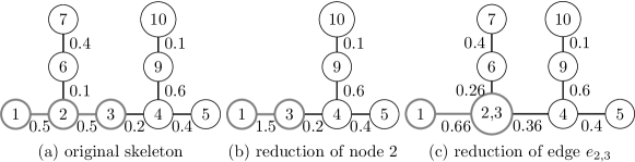
Figure 2: Different reductions of a path (in gray) within a skeletal tree.

Let us denote by $\kappa$ the function which applies the cheapest operation on a path. The successive applications of the function $\kappa$ associate to each path $h$ a sequence of reduced paths $(h,\kappa(h),\dots,\kappa^{D}(h))$ where $D$ denotes the maximal number of reductions. Using $K_{classic}$ for the path comparison, we define the kernel $K_{edit}$ as the mean value of kernels between reduced paths of equal length. Given two paths $h$ and $h^{\prime}$, this kernel is thus equal to $0$ if $||h|-|h^{\prime}||>D$. Indeed, in this case the maximal reduction of the longuest path remains longuer than the shortest one. Otherwise, $||h|-|h^{\prime}||\leq D$, and $K_{edit}(h,h^{\prime})$ is defined as:

$$K_{edit}(h,h^{\prime})=\frac{1}{D+1}\sum_{k=0}^{D}\sum_{l=0}^{D}K_{classic}(\kappa^{k}(h),\kappa^{l}(h^{\prime}))$$ (7)

This kernel is proportional (by a factor $D+1$) to a sum of $R$-convolution kernels [14, Lemma 1] and is thus definite positive.

Since $K_{classic}$ is equal to $0$ for paths of different lengths, $K_{edit}$ is indeed equal to a sum of kernels between reduced paths of equal length. For example, given two paths $h$ and $h^{\prime}$ whose respective length is equal to $4$ and $3$ we have for $D=2$:

$$\mbox{$K_{edit}$}(h,h^{\prime})=\frac{1}{3}\left[\mbox{$K_{classic}$}(\kappa(h),h^{\prime})+\mbox{$K_{classic}$}(\kappa^{2}(h),\kappa(h^{\prime}))\right]$$

4 Experiments

We used the following features for our experiments: Each node is weighted by its distance to the gravity center of the shape and each edge is assocated to a vector of two features: The first feature corresponds to the edge’s weight (section 3.2). The second feature is the angle between the straight line passing through the two nodes of the edge and the principal axis of the shape. These experiments are based on the LEMS [15] database which consists of 99 objects divided into 9 classes.

We defined three kernels for these experiments: The kernel $K_{max,classic}$ based on a conjoint use of the kernels $K_{max}$ (equation 2) and $K_{classic}$ (equation 4) has been introduced by Suard [6]. The kernel $K_{change,classic}$ based on a conjoint use of the kernels $K_{change}$ (equation 6) and $K_{classic}$ allows to evaluate the performances of the kernel $K_{change}$ compared to the kernel $K_{max}$. Finally, the kernel $K_{new}$ is based on a conjoint used of the two kernels $K_{edit}$ and $K_{change}$ proposed in this paper. The kernel $K_{classic}$ is defined by the two parameters $\sigma_{edge}$ and $\sigma_{vertex}$ respectively used by the Gaussian RBF kernels on edges and vertices. The kernel $K_{max,classic}$ does not require additional parameters while $K_{change,classic}$ is based on a $\nu$-SVM and requires thus the parameter $\nu$. It additionally requires the parameter $\sigma_{change}^{classic}$ used by the RBF kernel in  equation 6. The kernel $K_{edit}$ requires the two parameters $\sigma_{edge}$ and $\sigma_{vertex}$ used by $K_{classic}$ together with the maximal number of edition ($D$). Finally, the kernel $K_{new}$ requires as $K_{change}$ the two additional parameters $\nu$ and $\sigma_{change}^{new}$(equation 6). These parameters have been fixed to the following values in the experiments described below: $D=2$, $\sigma_{edge}=\sigma_{vertex}=0.1$, $\nu=0.9$, $\sigma_{change}^{new}=0.3$ and $\sigma_{change}^{classic}=1.0$. The parameters $\sigma_{edge}$ and $\sigma_{vertex}$ are common to all kernels. The remaining parameters have been been set in order to maximize the performances of each kernel on the experiments below.

Our first experiment compares the distance induced by each kernel $k$ and defined as $d^{2}(x,x^{\prime})=k(x,x)+k(x^{\prime},x^{\prime})-2k(x,x^{\prime})$. The mean number of matches for each class is defined as follows: For each shape of the selected class we sort all the shapes of the database according to their distances to the selected shape using an ascending order. The number of good matches of the input shape is then defined as the number of shapes ranked before the first shape which belongs to a different class than the selected one. For example, the $10$ nearest neighbors of a hand sorted in an ascending order are represented in Fig. 3(b), the number of good matches of each shape is indicated on the right of the figure. Note that the greater number of good match being obtained for the kernel $K_{new}$. The mean number of good matches of a class is defined as the mean value of the number of good matches for each shape of the class. The different values represented in Tab. 1(a) represent the mean values of these number of good matches for the classes: hands, tools and dudes (Fig. 3(a)). As indicated by Tab. 1(a), the kernel $K_{max,classic}$ provides stable results but is sensitive to slight perturbations of the shapes as the ones of the class dudes and cannot handle the severe modifications of the hands. The kernel $K_{change,classic}$ leads to roughly similar results on the different classes. Though not presented here, the kernel $K_{matching,classic}$ (equation 2.2) gives worst results than the others kernels. This result may be explained by the drawbacks of this kernel (Section 2.2). The kernel $K_{new}$ always provides the best results with a good robustness to perturbation on dudes and hands.

(a) hands,tools,dudes

(1)		$\eta=7$
(2)		$\eta=7$
(3)		$\eta=9$

(b) sorted distances to the hand

Figure 3: Five representative shapes of the classes hands, tools and dudes of the LEMS database (a), and (b) the 10 closest shapes from an hand using the distances induced by the kernels $K_{max,classic}$ (1), $K_{change,classic}$ (2) and $K_{new}$ (3).

	Hands	Tools	Dudes
$K_{max,classic}$	4.81	6.18	6.36
$K_{change,classic}$	5.27	5.45	6.36
$K_{new}$	7.09	9.82	6.36

(a) Mean number of good matches.

	Hands	Tools	Dudes
$K_{max,classic}$	7	11	10
$K_{change,classic}$	7	10	10
$K_{new}$	9	11	11

(b) Number of recognized shapes in one class.

Table 1: Kernels evaluation based on distance (a) and classification (b) criteria.

Our second experiment evaluates performances of each kernel within a classification framework. To this end, we have trained a SVM on 5 shapes of each of the three classes: dudes, hands, tools on one side and one model of each of the 6 remaining classes on the other side. The SVM margin parameter was selected in order to maximize the number of true positive while having no false positive. Tab. 1(b) shows the number of well classified shapes for each class. The kernel $K_{new}$ gives the best performances especially for the hands where the two missing shapes are the more perturbed ones. The two others kernels present good results and are competitive when shapes are not strongly deformed. This experiment confirms the robustness of our kernel against perturbed shapes.

5 Conclusion

The bag of path approach is based on a decomposition of the complex graph structure into a set of linear objects (paths). Such an approach benefits of recent advances in both string and vectors kernels. Our graph kernel based on a hierarchy of paths is more stable to small perturbations of the shapes than kernels based solely on a bag of paths. Our notion of path’s hierarchy is related to the graph edit distance through the successive rewritings of a path. Our kernel is thus related to the ones introduced by Neuhaus and Bunke.

References

- [1] Sharvit, D., Chan, J., Tek, H., Kimia, B.: Symmetry-based indexing of image databases. Journal of Visual Communication and Image Representation 9(4) (Dec. 1998) 366–380
- [2] Siddiqi, K., Shokoufandeh, A., Dickinson, S.J., Zucker, S.W.: Shock graphs and shape matching. Int. J. Comput. Vision 35(1) (1999) 13–32
- [3] Pelillo, M., Siddiqi, K., Zucker, S.: Matching hierarchical structures using association graphs. IEEE Trans. on PAMI 21(11) (Nov 1999) 1105–1120
- [4] Bunke, H., Riesen, K.: A family of novel graph kernels for structural pattern recognition. In: CIARP. (2007) 20–31
- [5] Neuhaus, M., Bunke, H.: Edit distance based kernel functions for structural pattern classification. Pattern Recognition 39 (2006) 1852–1863
- [6] Suard, F., Rakotomamonjy, A., Bensrhair, A.: Kernel on bag of paths for measuring similarity of shapes. In: European Symposium on Artificial Neural Networks, Bruges-Belgique (April 2007)
- [7] Haasdonk, B.: Feature space interpretation of svms with indefinite kernels. IEEE PAMI 27(4) (April 2005) 482–492
- [8] Desobry, F., Davy, M., Doncarli, C.: An online kernel change detection algorithm. IEEE TSP 53(8) (August 2005) 2961–2974
- [9] Kashima, H., Tsuda, K., Inokuchi, A.: Marginalized kernel between labeled graphs. In: In Proc. of the Twentieth International conference on machine Learning. (2003)
- [10] Ruberto, C.D.: Recognition of shapes by attributed skeletal graphs. Pattern Recognition 37(1) (2004) 21–31
- [11] Berg, C., Christensen, J.P.R., Ressel, P.: Harmonic Analysis on Semigroups. Springer-Verlag (1984)
- [12] Giblin, P.J., Kimia, B.B.: On the local form and transitions of symmetry sets, medial axes, and shocks. In: Seventh Internat. Conf. on Computer Vision. (1999) 385–391
- [13] Torsello, A., Handcock, E.R.: A skeletal measure of 2d shape similarity. CVIU 95 (2004) 1–29
- [14] Haussler, D.: Convolution kernels on discrete structures. Technical report, Department of Computer Science, University of California at Santa Cruz (1999)
- [15] LEMS: shapes databases. http://www.lems.brown.edu/vision/software/index.html