Eight-Dimensional Mid-Infrared/Optical Bayesian Quasar Selection

Abstract

We explore the multidimensional, multiwavelength selection of quasars from mid-IR (MIR) plus optical data, specifically from Spitzer-IRAC and the Sloan Digital Sky Survey (SDSS). Traditionally quasar selection relies on cuts in 2-D color space despite the fact that most modern surveys (optical and infrared) are done in more than 3 bandpasses. In this paper we apply modern statistical techniques to combined Spitzer MIR and SDSS optical data, allowing up to 8-D color selection of quasars. Using a Bayesian selection method, we catalog 5546 quasar candidates to an $8.0\mu$m depth of $56\mu$Jy over an area of $\sim 24$ deg². Roughly 70% of these candidates are not identified by applying the same Bayesian algorithm to 4-color SDSS optical data alone. The 8-D optical+MIR selection on this data set recovers $97.7$% of known type 1 quasars in this area and greatly improves the effectiveness of identifying $3.5<z<5$ quasars which are challenging to identify (without considerable contamination) using MIR data alone. We demonstrate that, even using only the two shortest wavelength IRAC bandpasses (3.6 and 4.5$\mu$m), it is possible to use our Bayesian techniques to select quasars with 97% completeness and as little as 10% contamination (as compared to $\sim$60% contamination using colors cuts alone). We compute photometric redshifts for our sample; comparison with known objects suggests a photometric redshift accuracy of 93.6% ($\Delta z\pm 0.3$), remaining roughly constant when the two reddest MIR bands are excluded. Despite the fact that our methods are designed to find type 1 (unobscured) quasars, as many as 1200 of the objects are type 2 (obscured) quasar candidates. Coupling deep optical imaging data, with deep mid-IR data could enable selection of quasars in significant numbers past the peak of the quasar luminosity function (QLF) to at least $z\sim 4$. Such a sample would constrain the shape of the QLF both above and below the break luminosity ($L^{*}_{Q}$) and enable quasar clustering studies over the largest range of redshift and luminosity to date, yielding significant gains in our understanding of the physics of quasars and their contribution to galaxy evolution.

1 Introduction

Enormous progress has been made in the last decade on understanding the nature of active galactic nuclei (AGNs) and their role in the lifecycle of galaxies. The co-evolutionary behaviour of black holes and spheroids, as implied by the $M-\sigma$ relation (e.g., Ferrarese & Merritt, 2000; Gebhardt et al., 2000; Tremaine et al., 2002), suggests that most massive galaxies hosted an AGN at some time. Indeed, energy injection from AGN through so-called “feedback” mechanisms (e.g., Silk & Rees, 1998; Fabian, 1999; Begelman, 2004; Hopkins et al., 2006) may be the linchpin connecting the blue, star forming and massive red, dead elliptical galaxies, whether through direct energy input (e.g., Ball et al., 2006; Croton et al., 2006), or as a somewhat more coincident product of the main quenching mechanism (e.g., major mergers could drive both AGN and quenching; Kauffmann & Haehnelt 2000; Hopkins et al. 2008).

Although feedback provides a key clue as to how galaxies evolve, there is a great deal of degeneracy in quenching prescriptions (e.g., Cattaneo et al., 2006). A promising avenue is constraining feedback models by examining the luminosity dependence to AGN clustering in combination with the AGN luminosity function (e.g., Lidz et al. 2006). However, current large quasar surveys typically track only the peak of the quasar luminosity function (QLF) at $z<2$ and only probe the brightest quasars at $z>3$, for example the Sloan Digital Sky Survey (SDSS; York et al. 2000) and the 2-Degree Field Quasar Survey (2QZ; Croom et al. 2004). Consequently, quasar clustering measurements (e.g., Porciani & Norberg, 2006; Myers et al., 2007; da Ângela et al., 2008) detect little luminosity dependence at $z<2$, and provide incomplete constraints at $z>3$.

If we wish to have a complete picture of the true role of feedback in quenching star formation and black hole growth in galaxies, then an important tool is to probe AGN (in statistically significant numbers) to luminosities below $L^{*}_{Q}$ at high redshift and below host galaxy depths at low redshift. In the long-term, the next generation of survey facilities such as LSST (e.g., Ivezic et al., 2008), Pan-STARRS (Kaiser et al., 2002), DES (The Dark Energy Survey Collaboration, 2005), and VST/VISTA (Arnaboldi et al., 2007), should produce sufficiently deep optical and near-IR photometry with which to address this goal. In the near-term, any sufficiently large-area survey of AGN that probes a wider luminosity range will blaze important observational and theoretical trails. This is particularly true of a large-area survey that contains the necessary color baseline (typically mid-IR through optical/UV) with which to simultaneously study AGN host galaxies at $z\lesssim 1$ and to characterize quasar photometric redshifts (e.g., Richards et al., 2001; Rowan-Robinson et al., 2008) out to $z\sim 3$ and beyond. As such, herein we describe a novel method for efficient selection of AGN from the combination of optical and mid-IR data that allows one to probe to the depths (and areas) that are required to compile the sort of data set that we have highlighted. As the existing overlap between SDSS and mid-IR imaging grows, so too will our ability to collect statistically significant samples of faint high-$z$ quasars that are needed to probe the influence of quasar feedback on galaxy evolution.

In principle, differentiating quasars from stars using mid-IR (MIR) colors is straightforward. At MIR wavelengths, stars (excepting the coolest brown dwarfs) are well-described by the Rayleigh-Jeans portion of a blackbody spectrum ($f_{\nu}\propto\nu^{2}$), resulting in quite blue colors, whereas quasars are much redder (steeper/softer; $f_{\nu}\propto\nu^{0\;{\rm to}\;-2}$). For MIR colors from Spitzer (Werner et al., 2004), it is not, in practice, quite this simple because Spitzer’s (comparatively) large pixels ($1\farcs 2$) makes it difficult to distinguish point from extended sources, and thus a simple color cut to select AGN suffers from considerable contamination from quiescent galaxies. However, judicious use of additional color cuts such as applied by Lacy et al. (2004a) and Stern et al. (2005) can be used to select quasars (both obscured and unobscured) with good efficiency and completeness for relatively bright MIR sources. See Donley et al. 2008 for a recent review of AGN selection techniques in the MIR.

In this paper we explore ways to improve upon color selection of AGNs using MIR colors. We particularly concentrate on 1) using sophisticated Bayesian selection methods, to probe to fainter limits (without additional contamination) than allowed by standard color selection, 2) incorporating optical morphology information, and 3) combining MIR and optical photometry, performing up to 8-D color selection. The latter approach increases completeness to high-redshift quasars (particularly $3.5<z<5.0$) where standard MIR color cuts are incomplete (or heavily contaminated). In addition, we will show that coupling deep optical and MIR data can overcome the loss of the two longest wavelength IRAC bandpasses when Spitzer’s coolant is depleted. Indeed, selection of quasars (both type 1 and type 2) and photometric redshift estimation for type 1 quasars suffer relatively little from this loss. Future coupling with deep UV, near-IR, and far-IR data from GALEX, UKIDSS, Akari, WISE, and Herschel will allow for further improvements in both selection and photometric redshift estimation.

We structure the paper as follows. § 2 describes our sources of data. We review our Bayesian selection algorithm in § 3, where we also describe the training sets designed for this selection. Application of our algorithm to combined SDSS and Spitzer data sets is discussed in § 4. The resulting catalog is presented in § 5. Obscured quasars are discussed in § 6 and we present our conclusions in § 7. Throughout this paper we report photometry either in flux density (in Jy) or AB magnitudes (denoted by square brackets). For the latter, Spitzer-IRAC Channels 1-4 are given by $[3.6]$, $[4.5]$, $[5.8]$ and $[8.0]$, which are the nominal wavelengths of the bandpasses in microns. The conversion between AB and Vega ($[{\rm Vega}]-[AB]$) is taken to be to be 2.779, 3.264, 3.748 and 4.382 mag for the four IRAC bandpasses. For example $[3.6]-[4.5]({\rm Vega})=[3.6]-[4.5]({\rm AB})+0.485$. Cosmology-dependent parameters are computed assuming $H_{o}=70\,{\rm km\,s^{-1}\,Mpc^{-1}}$, $\Omega_{m}=0.3$ and $\Omega_{\Lambda}=0.7$, in general agreement with the most recent WMAP results (Dunkley et al., 2008). Unless otherwise specified, the term “quasar” will refer to type 1 (broad-line) quasars/AGNs, regardless of their luminosity.

2 The Data

2.1 Samples

The selection methods described in this paper will make use of a variety of data sets. The MIR data are drawn from publicly available catalogs/images from all of the largest area Spitzer surveys using the Infrared Array Camera (IRAC; Fazio et al. 2004) where there exists overlap with optical data from the SDSS. We include Spitzer-IRAC data from the XFLS (Lacy et al., 2005); SWIRE (Lonsdale et al., 2003), specifically the ELAIS-N1, ELAIS-N2, and Lockman Hole fields; the NOAO-Boötes area from the IRAC Shallow Survey (Eisenhardt et al., 2004); and S-COSMOS (Sanders et al., 2007). The properties of these fields are summarized in Table 1. It is important to note that these Spitzer-IRAC data sets have very different depths, as indicated in Table 1. As the SWIRE data represent the largest fraction of objects in our analysis, we adopt their 95% completeness limit of 56$\mu$Jy at 8.0$\mu$m as the cutoff for our analysis. This choice excludes some high signal-to-noise data from the COSMOS field and keeps lower signal-to-noise data from the XFLS field, but is a good compromise for common analysis of all the data sets. The specific IRAC catalogs used are: XFLS (main_4band.cat; Lacy et al. 2005), SWIRE ELAIS-N1, -N2, and Lockman Hole (SWIRE2_N1_cat_IRAC24_16jun05.tbl, SWIRE2_N2_cat_IRAC24_16jun05.tbl, SWIRE2_Lockman_cat_IRAC24_10Nov05.tbl; Surace et al. 2005), and COSMOS (COSMOS_IRAC_0407_IRSA.tbl; Sanders et al. 2007). At the time of writing there were no publicly available MIR source catalogs for the NOAO-Boötes data, so we extracted photometry from the publicly available images when constructing the quasar training set; see § 2.3. In all there exists $\sim 32$ deg² of overlap between wide-area Spitzer fields and SDSS, with another $\sim 30$ deg² of SWIRE data lacking SDSS coverage.

Our primary goal herein is to perform 8-dimensional selection of quasars (primarily type 1) using optical and MIR data sets. The eight dimensions refer to the 8 unique colors afforded by SDSS $ugriz$ magnitudes (Fukugita et al., 1996) and Spitzer-IRAC Channel 1-4 flux densities. In addition, we perform 6-D selection of quasars using all 5 SDSS filters and the 2 short wavelength IRAC bandpasses (since the long wavelength bandpasses will not be available during Spitzer’s warm mission after its coolant is exhausted; Storrie-Lombardi et al. 2007). As such, we compile two combined MIR+optical data sets. One includes all objects detected in both IRAC Channels 1 and 2 that are matched to SDSS sources (95% completeness at $g=22.2$, $i=21.3$), for 6-D color classification. The second is a subset of the first where the objects are additionally detected in both IRAC Channels 3 and 4 (for 8-D color classification). IRAC upper limits are not considered as our selection algorithm is currently not equipped to handle them. Note, however, that the SDSS’s use of asinh magnitudes (Lupton et al., 2001) means that any object detected in one SDSS bandpass will have meaningful magnitude measurements in all the other bandpasses (even if they are nominally below the “flux limit”). Unless otherwise specified, all SDSS magnitudes herein are PSF magnitudes that have been corrected for Galactic extinction according to Schlegel et al. (1998).

2.2 SDSS-Spitzer Matching

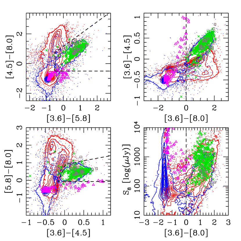
Figure 1: Comparison of MIR colors of point (blue contours/dots) and extended (red contours/dots) for various MIR color and flux combinations. Green points depicts known type 1 quasars, while open grey squares are type 2 quasars. Open magenta triangles indicate brown dwarfs (Patten et al., 2006). Comparison of these panels with Table 1 demonstrates that point sources with red MIR colors are robust AGNs candidates. The dashed lines depict the Lacy wedge region (upper left), Stern wedge region (lower left) and a simple $[3.6]-[8.0]$ color+morphology cut (right panels); see § 3. Statistical errors are generally less than 1%, but systematic errors can be $\sim 10$%.

Matching the combined 2-band IRAC data to the SDSS optical imaging catalog from the 6th SDSS data release (DR6; Adelman-McCarthy et al. 2007) with a $2\arcsec$ matching radius (IRAC has $1\farcs 2$ pixels and the median SDSS seeing is $\sim 1\farcs 3$) yields 324,618 objects. Of these, 486 objects are duplicates (243 pairs) where more than one SDSS source matched an IRAC source. To avoid any contamination, both objects in all of these duplicates were rejected. Spot checking of a few duplicates revealed that they tended to be galaxies that were improperly deblended in the SDSS. The 324,132 matches obtained after rejecting duplicates compose “Sample A”. Further limiting Sample A to objects detected in all 4 IRAC bands leaves 95,181 objects; we refer to this sample hereafter as “Sample B”. Sample B will be used for our 8-D classifications (and in the construction of our training sets). The MIR colors of Sample B are shown in Figure 1.

In Figure 1, the red contours/dots denote objects classified as extended sources, while the blue contours/dots are point sources. The extended vs. point-like classification is obtained on the basis of SDSS optical data by comparing PSF magnitudes with measures of extended flux for all bands in which the object is detected (Stoughton et al., 2002). For faint optical sources, star-galaxy separation begins to break down and galaxies become significant “stellar” contaminants. At $i\sim 20.8\;(S_{8\mu\rm m}\sim 115\mu{\rm Jy}$ at $z=1.5$ for a type 1 quasars), roughly 10% of SDSS point sources are likely to actually be galaxies.

The colors of the extended sources are concentrated in three clumps in Figure 1 (red contours/dots); understanding their origins is important for optimal object classification. The spectral energy distribution of extragalactic sources in the 1-8$\mu$m range is composed of three main components: (1) The combined light of stellar photospheres has a peak at 1.6$\mu$m (Sawicki, 2002) and declines according to the Rayleigh-Jeans law at longer wavelengths; (2) star-formation activity in the galaxy results in polycyclic aromatic hydrocarbon (PAH) emission from dust with strongest features at 3.3, 6.2, 7.7 and 8.6$\mu$m; and (3) circumnuclear dust may be heated by the central AGN resulting in continuum emission at MIR wavelengths, which is typically well-represented by a power-law since the dust is emitting at a wide range of temperatures. The relative contributions of these components to the total spectrum determines the IRAC colors of extragalactic objects. The colors of star-dominated and PAH-dominated galaxies at a wide range of redshifts (0–1.6) are quite distinct in the IRAC bands from the colors of the thermal emission of circumnuclear dust allowing color separation of AGNs from galaxies of all types. See Brodwin et al. (2006) and Donley et al. (2008) for more details regarding how galaxies track through MIR color space with redshift.

2.3 Quasars

In addition to matching the IRAC catalogs to the full SDSS optical catalogs, we have also explicitly matched it to the 77,429 spectroscopically confirmed quasars from the SDSS-DR5 quasar catalog Schneider et al. (2007). As the density of these known quasars is much smaller than the full SDSS object catalog, it is not too cumbersome to extract IRAC photometry from the publicly available IRAC images of Boötes field. While our Boötes data reduction was simplistic compared to the XFLS, SWIRE, and COSMOS data reductions, our analysis is substantiated by the lack of any difference in color as a function of redshift for the quasars in the Boötes region.

In all, matching the SDSS-DR5 quasar catalog to the IRAC data sets (again using a $2\arcsec$ matching radius) resulted in 425 matches. The relative IRAC and SDSS limits are such that all SDSS quasars are detected in the MIR. The additional 166 quasars as compared with Richards et al. (2006) come from the COSMOS and Boötes fields. We supplement these quasars with additional spectroscopically-confirmed quasars with both Spitzer-IRAC and SDSS photometry from Lacy et al. (2004a), Papovich et al. (2006), and Jiang et al. (2006), where the latter objects are $z\sim 6$ quasars and the two former samples were restricted to broad-line, type 1 AGNs. In all we have compiled 515 known type 1 quasars with both SDSS and IRAC detections; the MIR colors of these quasars are shown in Figure 1 as green points.

The SDSS-DR5 quasar catalog covers nearly all of the areas of overlap between SDSS and the SWIRE fields. Therefore, with the exception of several small-area fields and a part of the SWIRE/ELAIS-N1 area, these objects represent essentially all of the spectroscopically confirmed quasars that have been covered by both IRAC data and the final SDSS data release (DR7). The next major opportunity to obtain a large sample of spectroscopically confirmed quasars with MIR follow-up observations is with WISE (Mainzer et al., 2006), scheduled to launch in late 2009. WISE’s 120$\mu$Jy depth at 3.3$\mu$m will be sufficiently sensitive to detect all of the $i<19.1$ quasars in the SDSS catalog (but generally not the $z>3$ objects that extend as faint as $i=20.2$) and will significantly increase the number of quasars with MIR flux density measurements.

In addition to type 1 quasars, our selection is potentially sensitive to obscured (type 2) quasars. As such, it is important to know where type 2 quasars lie in the MIR+optical color space that we explore herein, so we have compiled a sample of type 2 quasars from literature with measured redshifts (either photometric or spectroscopic). These include samples from Zakamska et al. (2003, 291 objects); Reyes et al. (2008, 887 objects); Lacy et al. (2007c, 6 objects from XFLS); Lacy et al. (2007a, type 2 objects from Table 3, 30 objects from XFLS and SWIRE); Norman et al. (2002, one object at $z=3.7$); Mainieri et al. (2002, 20 objects from their Table 2, type 2 and unidentified objects (their type 9) with $\log(N_{H})>21.8$); Stern et al. (2002, one object at $z=3.288$); Sturm et al. (2006, 7 objects); Polletta et al. (2006, 125 objects); Tajer et al. (2007, 104 XMM-DS objects classified as AGN2 and starburst/AGN); Polletta et al. (2007, 21 objects from SWIRE/NDWFS/FLS, their Table 1 with redshifts from their Table 3); and Zheng et al. (2004, 141 objects from CDFS). We then matched this combined sample with all the available IRAC catalogs (including and in addition to those above) to extract Spitzer-IRAC photometry. Only objects detected at both 3.6$\mu$m and 4.5$\mu$m were selected in the matched output. This final output table was then matched to the SDSS DR6 catalog to select objects with both SDSS and Spitzer-IRAC photometry. This filtering/matching process was used to generate a final list of 43 type 2 quasars/candidates from literature with both SDSS and Spitzer-IRAC photometry. The MIR colors these type 2 quasars are given by open gray squares in Figure 1.

3 Bayesian Selection Overview

Our selection method follows that of Richards et al. (2004) and is detailed therein. For multi-band imaging surveys (such as the SDSS) it is possible to perform object classification beyond traditionally adopted 2-D color cuts. In particular, if the parameter space of interest is sufficiently populated by known objects, then these objects can be used as a “training set” to derive classifications within the parameter space (e.g., Hastie et al., 2001; Richards et al., 2004; Ball et al., 2006; Gao et al., 2008). Our algorithm of choice is based on kernel density estimation (KDE), weighted by a Bayesian “prior”. The KDE aspect is that the probability distribution function (pdf) that is used to evaluate the classification is smoothed by some appropriate kernel function (e.g., a Gaussian). Our algorithm uses two training sets, one that represents the objects to be classified and one that represents everything else. We compute the N-dimensional Euclidean color distance between some new object that we wish to classify and each of the training set objects. The new object is then classified based on how consistent its colors are with each training set (e.g., Gray et al., 2005). One limitation of our current algorithm is that error information is not explicitly included (cf., Ptak et al. 2007), although it is implicitly included by virtue of the training sets’ inherent error distribution.

Our Bayesian selection algorithm is guided by four considerations. First are the so-called “wedge” diagrams for MIR selection of AGNs. These are regions of color space that tend to be occupied by AGNs. Lacy et al. (2004a) select AGNs using color cuts in non-adjacent bandpasses to isolate AGNs, specifically $[3.6]-[5.8]$ and $[4.5]-[8.0]$; we refer to these color cuts as the “Lacy wedge”. Stern et al. (2005, 2007) instead utilize adjacent bandpasses, specifically $[3.6]-[4.5]$ and $[5.8]-[8.0]$; we refer to these color cuts as the “Stern wedge”. The exact color-cuts that describe these regions have changed slightly over time as more Spitzer data have been obtained. Thus we will refer to them in the abstract sense throughout the paper, but we visually illustrate them in Figure 1. The Lacy wedge region is given by the dashed lines in the top left-hand panel and the Stern wedge region is given by the dashed lines in the bottom left-hand panel.

The second diagnostic considers the mean colors for stars and quasars in the IRAC photometric system; Table 2 gives both the observed and theoretical (power-law approximated) values. For stars the $[3.6]-[8.0]$ color is $\sim-1.7$, while for quasars it ranges from $\sim 0$ to $1.7$. Thus, well-measured point sources can be grouped into stars and quasars in a straightforward manner, based on MIR colors alone.

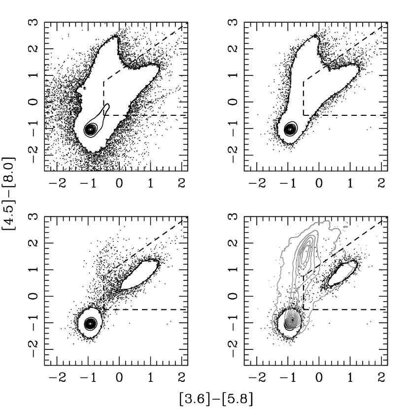
Figure 2: Illustration of the power of combining Spitzer data with morphology information. Top left: All 4-band data. Top-right: Removed very faint and saturated objects. Bottom-left: Limited to SDSS point sources. Bottom-right: Limited to SDSS point sources with $g<21.5$ (grey contours indicate extended sources). Dashed lines in each panel show the Lacy wedge. In short, MIR-only quasar selection is robust only for relatively bright sources or when coupled with accurate morphologies. Similar results would be seen for the Stern wedge (albeit with somewhat less contamination from galaxies at the price of reduced completeness to high-$z$ quasars).

Third, we consider the utility of having morphology information in addition to photometry and the effects of over-reliance on morphology as when star-galaxy separation fails to be robust. Figure 1 shows that AGNs are readily identified as point sources with red MIR colors (even using only the two shortest IRAC bandpasses). However, photometric errors complicate clean AGN identification at faint limits. Using just the Lacy wedge as an example, we demonstrate in Figure 2 how using a brighter MIR flux limit or morphology information can improve the efficiency of MIR color selection. Removing faint objects, saturated objects, and/or extended objects significantly reduces contamination.

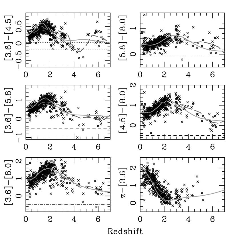
Figure 3: MIR colors of known broad-line, type 1 quasars (black x’s). The solid light gray and dashed dark gray curves show theoretical color redshift relation for a broad-band SED (Richards et al., 2006) and for the higher-resolution (Glikman et al., 2006) IR spectral template, respectively, the latter more accurately representing the effects of the H$\alpha$ emission line. In the upper two panels the dotted lines show the blue limits of the selection criteria for the Stern wedge (see Fig. 1, objects redder than these lines being inside the Stern wedge; the $[3.6]-[4.5]$ blue limit is a function of $[5.8]-[8.0]$, here only the extrema are plotted). In the middle two panels the dashed lines shows the same for the color combination used in the Lacy wedge (objects redder than these lines being inside the Lacy wedge). The bottom left-hand panel shows that, when coupled with morphology (see Fig 1), relatively complete and efficient selection is possible using only the $[3.6]-[8.0]$ color (dash-dot line). The bottom right-hand panels shows the 1$\mu$m inflection induced color change in $z-[3.6]$, which is extremely beneficial for photo-z’s.

Finally, we consider the color-redshift distribution for known quasars. Six color combinations are shown in Figure 3 as a function of redshift for the known quasar samples described above and for two template quasar spectra. The Stern (dotted) and Lacy (dashed) wedge color cuts (see Fig. 1) are included in order to show their effects on completeness with redshift. Cuts in $[3.6]-[4.5]$ can introduce incompleteness to $3.5<z<5.0$ quasars. The $z-[3.6]$ color changes rapidly between redshift 0 and 2 due primarily to a minimum in the SED, the so-called “$1\mu$m inflection” (e.g., Elvis et al., 1994).

3.1 Training Sets

The core of our quasar training set is the 515 optically-selected, spectroscopically-confirmed quasars that have existing Spitzer-IRAC photometry as discussed in § 2.3; this set is dominated by the 425 quasars from the SDSS-DR5 quasar catalog. Due to some photometric errors (bad deblending, etc.) objects with $[3.6]-[4.5]<-0.7$ or $[5.8]-[8.0]<-0.5$ are rejected. As our primary goal is efficient N-dimensional selection of type 1 (broad-line) quasars, we have not explicitly included obscured or intrinsically weak AGNs in the training set, although doing so would be a logical next step for future investigation.

Since the number of known quasars with optical and MIR photometry is relatively small in comparison with the size of the sample that we wish to classify, we further include IRAC 4-band matches to SDSS sources that are highly likely to be quasars. Below we describe two such classes of objects that are included. For these samples to be as clean as possible, we require that the sources satisfy $56\mu{\rm Jy}<f_{8.0\mu{\rm m}}<10{\rm mJy}$, and $i>14.0$ to exclude saturated objects and to limit the samples to the approximate 8.0$\mu$m 95% completeness limit of the SWIRE data.

First, given the power of combining morphology with MIR colors shown in Figure 2, we identify point sources with red (AGN-like) MIR colors as quasar candidates that are sufficiently robust to be included in the training set. As SDSS star-galaxy separation begins to break down at faint magnitudes ($r\sim 21$; Scranton et al. 2002) with faint extended sources being more likely to be classified as point-like, clean point source identification should be restricted to $i\lesssim 20.8$ (0.5 mag brighter than the nominal SDSS $i$-band flux limit). Thus, point sources with $i<20.8$ are classified as quasars if they have $[3.6]-[8.0]>0$, see Table 1. However, for the XFLS data, the MIR photometric errors are large enough that a simple cut in $[3.6]-[8.0]$ is insufficient to cleanly identify quasars; for these objects we also require $[3.6]-[5.8]>-0.5$ and $[4.5]-[8.0]>-0.5$ (akin to the Lacy wedge). Finally true point source quasars do not typically have MIR colors outside of $-0.4<[5.8]-[8.0]<1.4$ and $[3.6]-[4.5]<-0.6$, so we exclude such objects to further limit any contamination by misclassified galaxies and by normal stars.

Second, in addition to the above red MIR point sources, we capitalize on the work of Lacy et al. (2004a) and Stern et al. (2005) by including objects that can be robustly identified as quasar candidates based on their location in the MIR wedge diagrams. While selection using these wedges is relatively clean at bright limits, the colors of quasars may change with flux (indeed Fig. 1 suggests that at fainter limits the quasar contribution weakens with respect to the galaxy contribution, making the MIR colors bluer on average), thus additional constraints are needed to exclude contaminants. In particular, we include in the quasar training set any point sources that are in any of 1) the Lacy wedge, 2) the Stern wedge, or 3) a modified Stern wedge (which excludes a region near the galaxy locus, see § 3.2 below). We further include extended sources that lie in both the Lacy wedge and our modified Stern wedge. In addition to relatively robust MIR point source candidates, these criteria select point sources near the quasar/galaxy boundary in $[3.6]-[4.5]$ (between the original and modified Stern wedges), but reject extended sources in this same “buffer zone” where it may be difficult to distinguish true galactic contaminants from host-dominated quasars.

For these two MIR-selected training set populations, we have not utilized any optical magnitude or color information since optical quasar selection is known to be incomplete in certain redshift ranges (e.g., $z\sim 2.7$, Richards et al. 2006), and the inclusion of these MIR-identified sources is our attempt to mitigate this effect. However, roughly half of these objects are UV-excess sources that would be included using optical selection alone. Similar to the $z\sim 2.7$ redshift incompleteness in the optical, MIR-only selection is incomplete in a different redshift range ($3.5<z<5$), thus the inclusion of optical-only selection objects in the training set helps recover such objects in our higher dimensional selection. Having a training set comprised of both optical-only (the above 515 known quasars) and MIR-only identified sources aids in the creation of a photometric quasar sample that is as complete as possible at all redshifts. While no MIR-only or optical-only quasar samples are fully complete at all redshifts, by combining the two and then performing quasar selection simultaneously on both MIR and optical colors, we overcome the limitations inherent to each method separately.

Due to photometric errors (bad deblending, etc.), a handful of the quasar training set objects are outliers from the quasar color-redshift distribution. We only retain objects that are in the intersection of the following criteria: $[3.6]-[8.0]>-0.5$, $[3.6]-[4.5]>-0.5$, $[4.5]-[5.8]>-0.7$, and $[5.8]-[8.0]>-0.5$. In summary, the final quasar training set is the combination of 1) known quasars, 2) red MIR objects with point-like optical morphologies, 3) point/extended sources identified in two distinct MIR color wedges, and 4) excluding some photometric error induced outliers and some extended sources on the border between known quasars and galaxies.

As was the case for our purely optical selection (Richards et al., 2004), a more difficult task is to define the non-quasar training set (here both stars and normal galaxies) as we do not have a sufficiently large (and representative) sample of spectroscopically confirmed objects. While there are many thousands of SDSS spectra of galaxies and stars, the galaxy sample extends only to $r=17.77$ and the star spectra cover only specific regions of color parameter space. Furthermore, optical spectra may not reveal the AGN nature of a galaxy as well as the MIR colors would. Thus, we are essentially left with identifying the leftovers from our quasar training set as the non-quasar training set, with the exception of borderline objects that we exclude from either training set. Objects in the non-quasar training set satisfy the following conditions. First, they must not be in the quasar training set. Second, they are rejected if they lie in the Lacy wedge and also either the original or modified Stern wedges. The remaining objects that meet our magnitude and flux limits constitute the non-quasar training set.

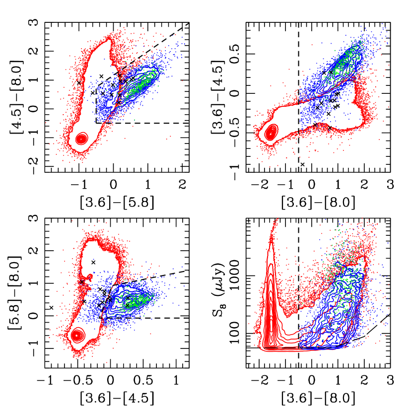
Figure 4: MIR color-color and color-mag distributions for the quasar (blue contours/dots) and non-quasar (red contours/dots) training sets. Green points indicate known quasars; black crosses mark $z>3.5$ quasars. The long dashed line in the bottom right-hand panel shows our adopted $8.0\mu$m flux limit and how it is affected by the $3.6\mu$m and $5.8\mu$m limits.

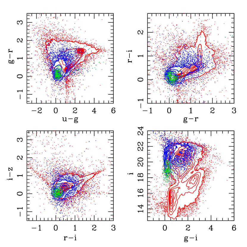
Figure 5: SDSS color-color and color-mag distribution for the quasar (blue contours/dots) and non-quasar (red contours/dots) training sets. Green points indicate known quasars.

Figure 4 shows the MIR color distribution of the objects in the quasar and non-quasar training sets. The SDSS colors of the same objects are shown in Figure 5. The training set has 53332 objects; 5627 labeled as quasars and 47705 as non-quasars. For our Bayesian classification method, we need to estimate a “prior” that indicates the a priori probability of any given object in our samples not being a quasar. We adopt the fraction determined from the training sets as a reasonable value, specifically 89%.

3.2 The Modified Stern Wedge Region

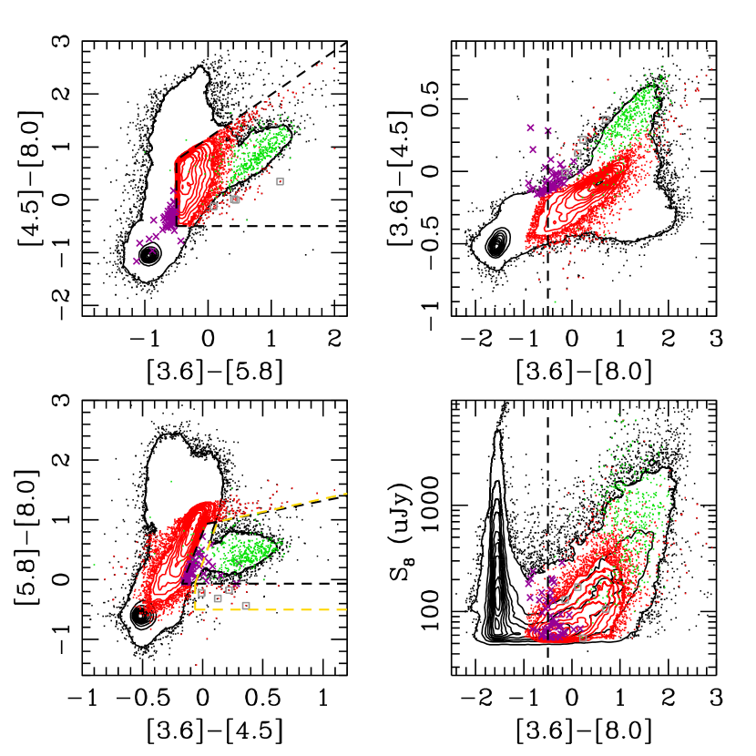
Figure 6: Comparison of the two standard MIR “wedge” color selection algorithms. The top left panel shows that of Lacy et al. (2004a) (dashed lines). The bottom left panel that of Stern et al. (2005), again as dashed lines. Black contours and dots are all sources detected in all 4 IRAC bands that have matches to SDSS sources. Green points indicate known quasars. Red contours/dots show objects inside the Lacy wedge, but outside the Stern wedge. Purple crosses indicate objects in the Stern wedge, but outside the Lacy wedge. The right panels show additional regions of color-color and flux-color space. The dashed line in the right-hand panels indicates a logical dividing line between stars and AGNs among point sources. The region enclosed by yellow dashed lines in the lower left-hand panel indicates our modified Stern wedge, which is more conservative on the galaxy/AGN boundary in $[3.6]-[4.5]$, but is more inclusive to potential AGNs that have blue $[5.8]-[8.0]$ colors. Open grey squares indicate the colors of 3 confirmed and one likely AGN resulting from spectroscopic follow-up of 9 random sources with $[5.8]-[8.0]<-0.07$.

In Figure 6 we compare and contrast the two primary MIR color selection techniques in use today; see also Donley et al. (2008). By exploring the color space occupied by objects selected by the Stern wedge, but not the Lacy wedge, and vice versa, we hope to create a more robust quasar training set from MIR colors. Examination of Figure 6 reveals the following

• The Stern wedge is relatively clean (few objects are outside of the Lacy wedge).

• The Lacy wedge is very clean to the 1 mJy flux limit for which it was defined but is quite contaminated at fainter MIR fluxes (it contains many objects outside of the Stern wedge).

• The Stern wedge’s lack of contamination comes largely from its cut on $[3.6]-[4.5]$. Although very effective over a wide range of redshifts, this cut makes the Stern wedge incomplete to quasars with $3.5<z<5.0$ (see Fig. 3).

Furthermore, we note that the Stern wedge’s blue cut in $[5.8]-[8.0]$ excludes objects that are in the Lacy wedge. Such objects are rejected nominally to exclude high-redshift galaxies (see Fig. 1 in Stern et al. 2005); however, as these objects are found by Hickox et al. (2006) to be strong soft X-ray sources, the AGN population likely crosses this dividing line.

Indeed, during a 2008 June observing run on the Mayall 4-m telescope at Kitt Peak National Observatory, we were able to make observations of 9 randomly chosen sources blueward of the Stern wedge’s $[5.8]-[8.0]$ cut. Of the six sources redder than $[3.6]-[4.5]=-0.1$, three are clearly quasars ($z=0.91,1.61,1.64$) and a 4th may also be a quasar at low signal-to-noise; their MIR colors are shown in Figure 6.

These objects are all in the region of strong soft X-ray sources (and thus likely quasars) as indicated by Hickox et al. (2006) and have two similar features. All are flagged as color selected quasar candidates (Richards et al., 2002) in the SDSS database, but were too faint to be targeted for spectroscopy. They also have very similar appearances in the optical, being extended, but centrally concentrated bluish-white objects. When coupled with MIR data, these characteristics may help to identify additional quasars in the SDSS database that are nominally outside of the Stern wedge, but that may nevertheless be AGNs.

Thus, as mentioned above, we implement a “modified Stern wedge” that is adjusted from the original Stern wedge as follows. We first make a more conservative cut on the AGN/galaxy border in $[3.6]-[4.5]$ color. Second, we allow objects bluer than $[5.8]-[8.0]<-0.07$ if they have $[3.6]-[4.5]>-0.0626$ (the intersection of our modified $[3.6]-[4.5]$ and the original $[5.8]-[8.0]$ cuts). This modified Stern wedge is defined by the following set of color cuts (see Fig. 6)

$$(([5.8]-[8.0])>-0.07\;\&\&\;([3.6]-[4.5])>0.18*([5.8]-[8.0])-0.05\;\&\&$$

$$([3.6]-[4.5])>2.5*([5.8]-[8.0])-2.295)\;||\;$$

$$([3.6]-[4.5]>-0.0626\;\&\&\;(-0.5<[5.8]-[8.0]\leq-0.07)).$$ (1)

No modifications have been made to the Lacy wedge because coupling it with the Stern wedge already removes spurious sources. We are not suggesting that this modified wedge be used in place of the Stern wedge for MIR AGN selection, rather we use it to minimizing contamination from normal galaxies in our training sets, while attempting to maximize completeness to quasars with $3.5<z<5$.

4 Application of the Algorithm

Once the training sets are defined, we follow the techniques described in Richards et al. (2004) for utilizing these training sets to select objects from a sample of data. We shall perform this selection for two sets of color space: 8-D (MIR+optical) to attempt a more complete type 1 quasar selection than can be accomplished with MIR-only or optical-only selection; and 6-D, anticipating the operation of Spitzer post-cryogen, when only IRAC Channels 1 and 2 will be operational. We have additionally attempted a 3-D MIR-only Bayesian selection. Although this approach adds an extra color dimension that is otherwise being wasted by the 2-D MIR wedge selection methods, we find that it does not work significantly better (e.g., it is still rather incomplete to $3.5<z<5.0$ quasars as is the Stern wedge) and do not discuss it further here.

In addition to a prior (as discussed above) our algorithm also uses a leave-one-out cross-validation process to determine the optimal bandwidths (kernel smoothing parameter) for the AGN and non-AGN samples, respectively. These bandwidths are essentially the resolution of the pdf, akin to the bin size for a histogram. See Richards et al. (2004) for details, but, in brief, the algorithm examines a range of bandwidths and chooses the one that maximizes our completeness to known quasars while minimizing contamination. The adopted training set bandwidths notated as (star, quasar) were $(0.2,0.11)$ and $(0.195,0.05)$ magnitudes, for the 8-D and 6-D selection, respectively. The selection is reasonably robust to small ($\sim 0.05$ mag) changes from these values.

4.1 8-D

Quasar selection is essentially an algorithm that identifies outliers from the stellar locus in the optical or the galaxy locus in the MIR. Thus, one might expect that combining optical and MIR photometry together will yield more robust quasar selection than optical or MIR photometry alone as objects only need to be outliers in one dimension. In particular, our desire is to combine the 5 SDSS and all 4 IRAC bandpasses together to recover the $2.5<z<3.0$ quasars lost by optical selection due to stellar locus contamination and the $3.5<z<5.0$ quasars lost by MIR selection due to galaxy locus contamination.

We have applied our Bayesian selection method to the 8 unique colors afforded by SDSS plus IRAC photometry in Sample B. As with the training sets, we limit Sample B to $56\mu{\rm Jy}<f_{8.0\mu{\rm m}}<10{\rm mJy}$, and $i>14.0$, which reduces the sample from 95,181 objects to 52,659 objects. In all, 5468 quasar candidates were found.

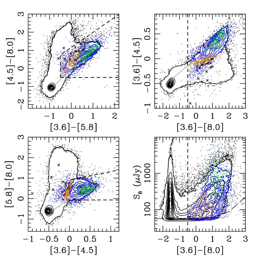
Figure 7: MIR colors/flux densities of Bayesian selected quasars. Black contours/dots show the full sample. Blue contours/dots show objects selected by both the 8-D and 6-D Bayesian algorithms. Gold (red) points are objects selected only by the 8-D (6-D) algorithm. Known quasars are shown in green with $z>3.5$ quasars shown by black crosses. Theoretical power-law colors ($-2<\alpha_{\nu}<2$) are given by the grey line (where we assume a delta function filter curve at the nominal effective wavelength). Deviations from power-laws are seen in the Stern wedge due to the use of adjacent bandpasses where the small-wavelength structure can dominate the overall shape of the MIR SED.

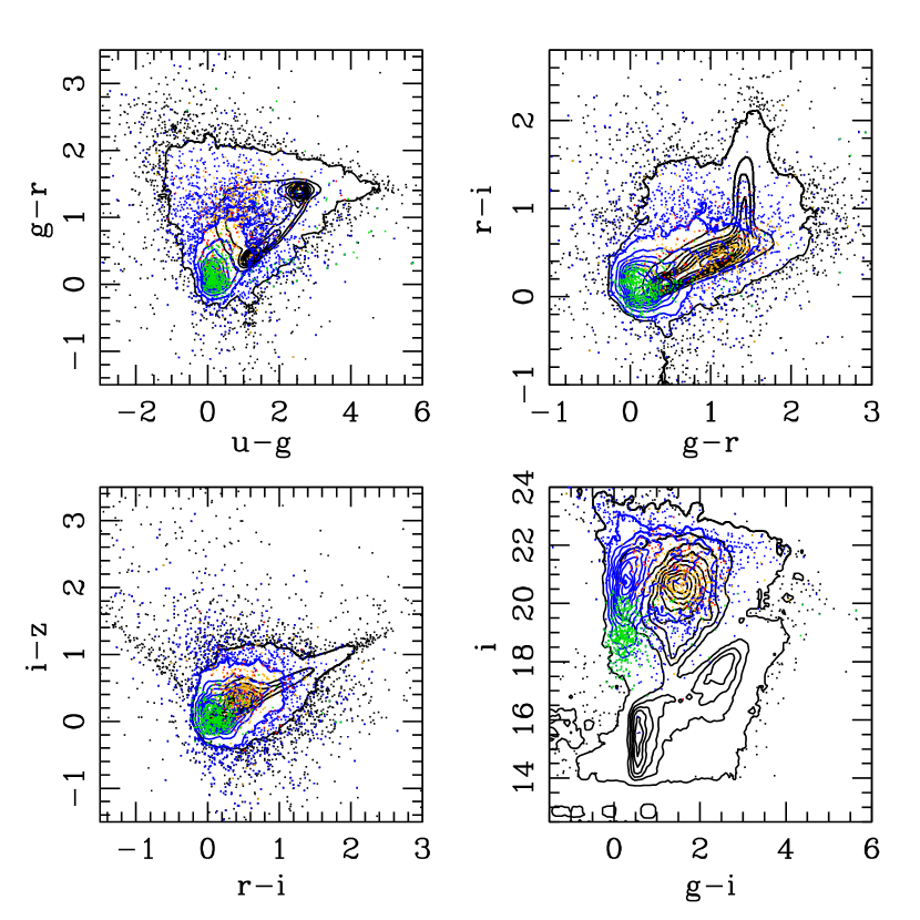
Figure 8: Optical colors/mags of Bayesian selected quasars. Black contours/dots show the full sample. Blue contours/dots show objects selected by both the 8-D and 6-D Bayesian algorithms. Gold (red) points are objects selected only by the 8-D (6-D) algorithm. Again, known quasars are shown in green.

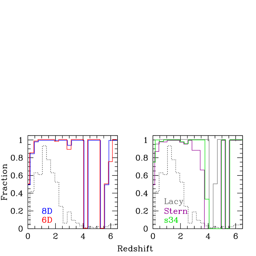
Figure 9: Fraction of known (type 1) quasars recovered. Left: Our 8-D (blue) and 6-D(red) Bayesian selection algorithms. Right: The Lacy wedge (gray), the Stern wedge (purple) and a $[3.6]-[4.5]$ color cut (green). The dashed black line in each panel indicates the number of known objects in each redshift bin. The peak at $z=1.2$ has 89 objects. $z=5.4$ has 0 objects and $z=4.2$ and $z=4.8$ have only one each, thus statistics are poor in these bins.

The MIR and optical color distributions of these 8-D selected objects are shown in Figures 7 and 8, respectively. Here we have added theoretical power-law colors to the MIR color-color plots, which demonstrates that the most robust objects tend to have power-law colors in the MIR (e.g., Donley et al., 2008). The primary differences between these and 2-D MIR wedge selection are that 541 objects outside of the Stern wedge are now selected and the left (blue) part of the Lacy wedge is more represented. The redshift completeness (to known type 1 quasars) is given in the left-hand panel of Figure 9. As compared to MIR-only selection using the Stern wedge (right-hand panel), it is clear that that 8-D MIR+optical selection performs better over $3.5<z<5$. Overall the completeness to spectroscopically confirmed type 1 quasars is 97.7%. This high completeness suggests that it should be possible to attempt to classify fainter sources and still maintain a reasonably high completeness — although clearly photometric errors limit how faint the method can be applied.

4.2 6-D

These results from our 8-D Bayesian selection are promising; however, once Spitzer has exhausted its coolant, it will no longer be able to observe in the two longest IRAC bands. Thus an interesting question is how well our methods will work when only IRAC Channels 1 and 2 are operational.

As such, we have also performed a 6-D Bayesian selection using the 5 SDSS bandpasses and only the 2 shortest wavelength IRAC bandpasses. Instead of using Sample A here (which includes object rejected from Sample B due to lack of Channel 3/4 detections), we instead have only considered the same 52,659 magnitude/flux-limited sources from Sample B above, simply ignoring the color information from Channels 3/4. We have made this choice in order to provide the most direct and unbiased comparison between 8-D and 6-D selection. However, we emphasize that, similarly limiting sample A to unsaturated sources and the SWIRE 95% completeness limit at 3.6$\mu$m (Table 1) [allowing non-detections in Channels 3/4], we can potentially apply our 6-D algorithm to over 290,000 sources.

Overall our 6-D algorithm selects 5222 objects and is not significantly worse than 8-D, with a completeness of 97.1% with respect to the type 1 quasars in the training set. The completeness as a function of redshift (red line in the left-hand panel of Fig. 9) is consistent with that for 8-D selection. The drop in $z>5.5$ completeness is not statistically significant given the small number of objects considered. In all, 324 (6%) objects that were selected by the 8-D algorithm are not 6-D candidates. There are also 78 (1%) 6-D selected sources that are not 8-D candidates. Figures 7 and 8 show the locations of objects selected by both the 8-D and 6-D algorithms and also those selected by only one.

4.3 Comparison of Selection Methods

Table 3 shows a comparison between our Bayesian selection methods, the Lacy and Stern wedges, and a simple $[3.6]-[4.5]>-0.1$ color cut. For bright flux limits ($f_{8.0\mu{\rm m}}>1\,{\rm mJy}$) our Bayesian method agrees well with the Lacy and Stern wedges, with the $[3.6]-[4.5]>-0.1$ cut being about 50% contaminated. At fainter limits the Lacy wedge is seen to be contaminated by inactive galaxies, the $[3.6]-[4.5]$ cut somewhat less so. Of 8-D Bayesian selected quasars candidates, 99% are within the Lacy wedge and 90% are within the Stern wedge; thus we expect the Bayesian sample to be quite clean.

In terms of completeness, Figure 9 demonstrates that the Lacy wedge and either of our 8-D or 6-D Bayesian algorithms are quite complete to type 1 quasars at nearly all redshifts. The comparison sample is the set of spectroscopically-confirmed type 1 quasars that were used to construct our quasar training set. Thus, Figure 9 represents the self-selection completeness. As an additional check, we find that our algorithm recovers all 51 of the type 1 quasars cataloged by Trump et al. (2007) in the COSMOS field (to $i<21.3$ and $f_{8.0\mu{\rm m}}<56\,\mu$Jy). The Lacy wedge is much more contaminated (Table 3) than our Bayesian-selected samples. The Stern wedge would appear to be the least contaminated, but is also the least complete, particularly for $3.5<z<5.0$. A simple $[3.6]-[4.5]$ color cut is somewhat more complete than Stern wedge selection, but suffers from considerable contamination. While a $[3.6]-[8.0]$ color cut might be expected to be cleaner than $[3.6]-[4.5]$, the presence of PAH features at $8\mu$m causes contamination from low-redshift PAH-dominated galaxies that overwhelms the loss of stellar contaminants due to the longer baseline.

A particularly interesting question is how well our MIR+optical selection performs above optical-only selection algorithm. For this comparison, we utilize our optical-only Bayesian-selected quasar catalog (Richards et al., 2008), which includes unresolved SDSS quasar candidates to the nominal SDSS magnitude limit of $i<21.3$. We find that 1702 of 2426 (70%) of our optical+MIR selected targets are also selected by the optical-only algorithm (for $i<21.3$ point sources). However, our MIR+optical selection benefits by adding 2117 extended sources and 1003 points sources with $i>21.3$ (i.e., nominally fainter than the SDSS magnitude limit). Thus, using the same SDSS dataset as a basis, our MIR+optical selection improves quasar selection by a factor of 3.25 (5546/1702).

It is instructive to consider the future of MIR-based selection of quasars in general, even without the benefit of our Bayesian selection method. Indeed, while the wedge selection methods rely on IRAC Channels 3 and 4, it is actually Channels 1 and 2 that are most needed — in terms of separating AGNs from stars and normal galaxies. As can be seen in Figure 1, in the absence of accurate morphological classification, quasars selected with a $[3.6]-[4.5]$ cut will have less contamination from galaxies than a $[3.6]-[8.0]$ cut, yet be similarly effective in removing stars. Using a $[3.6]-[4.5]$ color cut alone, we find that for $[3.6]-[4.5]>0.1$, 91% of known quasars are recovered. Relaxing the cut to $[3.6]-[4.5]>-0.1$ recovers 98% of quasars, although the missing objects are predominantly high-$z$. However, we must also consider the level of contamination. Figure 10 shows the tradeoff between (type 1) completeness and contamination. Here we have made the simplifying assumption that any object lying outside either the Lacy and Stern wedges are not quasars and that objects lying inside both the Lacy and Stern wedges are quasars. For $[3.6]-[4.5]>-0.1$ the contamination fraction is nearly 60%, though we caution that this number depends significantly on the flux limit. More importantly, if we desire to recover all of the high-$z$ quasars, we must instead use $[3.6]-[4.5]>-0.4$, which has over 85% contamination. On the other hand, our 6-D Bayesian selection (which also uses only Channels 1 and 2) is 97.1% complete to known type 1 quasars (including high-$z$), with only 10% contamination, using the same criteria.

5 Catalog

Our catalog is presented in Tables 4 and 5, where Table 4 describes the columns in Table 5. For the sake of completeness, we also tabulate the 593 objects that were not selected by our Bayesian algorithms but that otherwise meet our flux/magnitude criteria and are in both the Lacy and Stern wedges; these objects are given in Table 6. The numbering of objects is common to Tables 5 and 6 and are sorted by right ascension.

The first 25 columns in the data tables merely repeat the publicly available optical and MIR information on these sources, see Adelman-McCarthy et al. (2008) and the references above for more information. Columns 26–30 deal with object selection as discussed in § 4. Columns 31–38 give photometric redshift information as discussed in the next section. Columns 39-41 provide information on previous identification of these objects, whether photometric (Richards et al., 2008), or spectroscopic (DR5x, Schneider et al. 2007; DR6x, Adelman-McCarthy et al. 2008; T07x, Trump et al. 2007; P06x; Papovich et al. 2006). For the spectroscopic identifications we have simply repeated the classifications from the indicated references.

In all there are 5546 objects cataloged in Table 4. Note that this number is similar to the number of objects in our quasar training set. This similarity is a result of our using the same flux limit for both our training and test sets, while we could have performed 6-D selection to much fainter limits (nearly 6$\times$ as many objects). As we consider our work here to be a “proof-of-concept”, we save fainter 6-D quasar selection as an exercise for the future after the current catalog has been more fully validated with spectroscopic observations.

Thus our procedure has essentially thrown out some wedge-selected quasar candidates and has included some objects outside of the quasar color wedges in the MIR. That this is a worthwhile process can be seen by noting that quasars make up 92% of the known objects in among our Bayesian selected targets (Table 5), while the fraction of quasars among our rejected targets (Table 6) is only 29%. In addition, our Bayesian algorithm was shown to be more robust than MIR-only color section over $3.5<z<5.0$ (Fig. 9), and is less contaminated at fainter flux limits (Table 3). These properties will be particularly beneficial to the deeper census that can be performed with objects detected in only the 2 bluest IRAC bandpasses.

5.1 Photometric Redshifts

While the errors on the IRAC flux densities ($\sim 10$% for IRAC [but see Hora et al. 2008] vs. $\sim 2$% for SDSS) are generally too large to permit accurate MIR-only photometric redshift estimation, the combination of SDSS and IRAC photometry allows for considerable leverage in estimating redshifts of AGNs. We have updated the algorithm described by Richards et al. (2001) and Weinstein et al. (2004) to operate on any number of color dimensions. In essence, quasar photometric redshift estimation relies on the small, but distinct, color changes produced as broad emission lines move through photometric bandpasses. At $z\gtrsim 2.3$, Lyman-$\alpha$ forest absorption mimics the Balmer break that is so useful in reducing galaxy photometric redshift estimates to the 2% level (e.g., Connolly et al., 1995). However, quasar emission lines are generally strong enough that they also produce measurable features in the color-redshift relations that can be used to estimate photometric redshifts (photo-$z$’s). The mean SDSS colors as a function of redshift were shown most recently by Schneider et al. (2007), while the redshift dependence of IRAC colors for SDSS quasars was given by Hatziminaoglou et al. (2005) and Richards et al. (2006, Fig. 3); see also Figure 3.

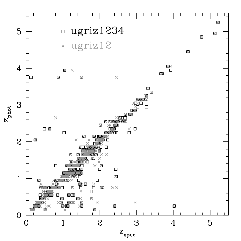
Figure 11: Left: Photometric vs. spectroscopic redshift for 399 known quasars. Open black squares show photometric redshifts determined from 8 colors. Grey crosses show photometric redshifts determined from 6 colors. Right: Histogram of the fractional error in photometric redshift. 8-color photo-z results are shown by the solid line; 6-color by the dashed line. Little accuracy is lost by going from 8 to 6 colors. The bin size is 0.05 in redshift.

Using the IRAC-detected, spectroscopically-confirmed quasars noted above, we have updated the quasar color-redshift relations and computed the photometric redshifts for all of our quasar candidates. In addition, Table 4 provides not only the most likely photometric redshifts, but also a range and the probability that the actual redshift is within that range. We compute photometric redshifts both using both 8 colors and 6 colors (dropping the 2 reddest IRAC bandpasses to simulate the Spitzer warm mission data). In the left-hand panel of Figure 11, we show both the 8-D and 6-D photometric redshifts versus spectroscopic redshifts. The 6-color photo-z’s are not significantly worse than the 8-color photo-z’s. This is perhaps not surprising given that most of the information that comes from adding the IRAC bandpasses is provided by the $z-[3.6]$ color which, due to the 1 micron inflection, spans an impressive 2 magnitudes over $0<z<2$ (see the bottom right-hand panel in Fig. 3) and serves to break most of the redshift degeneracies seen when computing photometric redshifts from SDSS photometry alone. Within $\pm 0.3$ in redshift, we find that both the 8-color and 6-color photo-z’s are accurate 93.6% of the time. In addition, the majority of the photo-z’s are considerably more accurate than $\pm 0.3$; 82–84% are accurate to $\pm 0.1$ in redshift. This accuracy is illustrated in the right-hand panel of Figure 11, where we show a histogram of the fractional redshift errors. Most of the outliers are fainter objects with $i>19.1$, but even for those the fraction of 6-color photoz’s accurate to $\pm 0.3$ is 92%.

In principle, any deep optical imaging data can be used to determine photometric redshifts, but in practice the SDSS filter set is nearly ideal for photometric redshifts of quasars due to the more “top-hat” nature of the SDSS filters than the traditional Johnson-Morgan/Kron-Cousins filters. We emphasize that our goal here is primarily to find type 1 quasars for which our photometric redshift algorithm should work quite well. However, at faint flux limits and/or larger host galaxy contribution, our templates fail to yield accurate photo-z’s — necessitating more careful photometric redshift techniques. For example, if the multi-wavelength coverage is large enough (e.g., UV, optical, near-IR, and MIR), it is also possible to determine photometric redshifts through SED template fitting (e.g., Brodwin et al., 2006; Rowan-Robinson et al., 2008; Salvato et al., 2008) which also enables simultaneous photometric redshift estimation for inactive galaxies and type 2 quasars.

5.2 Bulk Properties

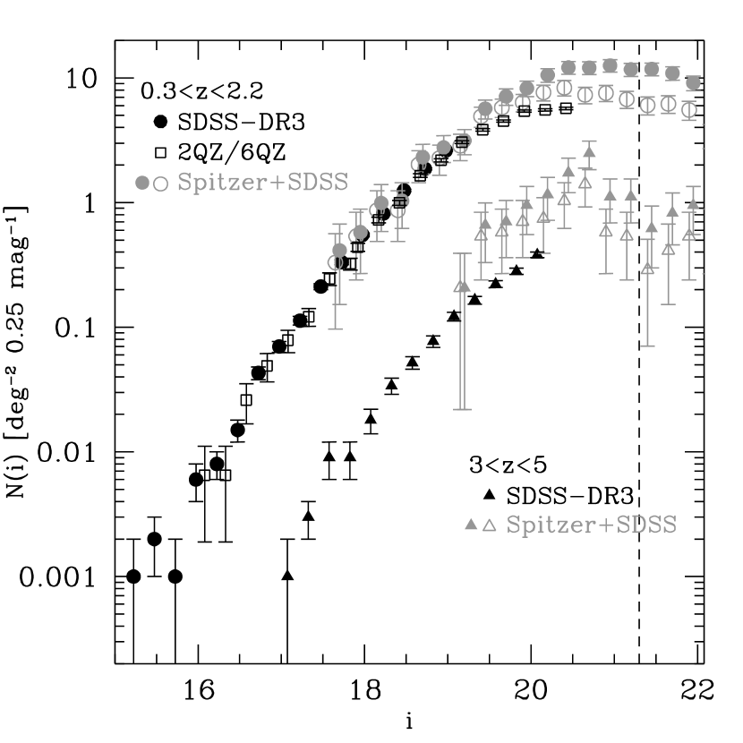
Figure 12: Number counts ($i$-band) of Spitzer+SDSS selected quasars as compared to SDSS and 2QZ number counts. Two redshift bins are shown: $0.3<z<2.2$ as circles/squares and $3<z<5$ as triangles. Our new results are shown for two extreme cases: objects selected by either the 6-D or 8-D algorithms and with photometric redshift probability larger than 0.5 (closed points) and for objects selected by both the 6-D and 8-D algorithms and with photometric redshift probability larger than 0.8 (open points). For objects brighter than the nominal SDSS flux limit of $i=21.3$, these extremes should bracket the true values. Points are truncated at the bright end where the errors become large due to the lack of area.

With the aid of photometric redshifts, we can examine other properties of the catalog. Figure 12 shows the number counts of our sample as compared to the SDSS-DR3 (Richards et al., 2006) and 2QZ results (Croom et al., 2004). Two extreme cuts on our catalog are shown to give the reader the range of possible values as objects get fainter and classification (and redshift estimation) become less robust. The number counts are just slightly above those of the SDSS spectroscopic sample for relatively bright $z<2.2$ sources, which is consistent with the fact that fully or partially obscured quasars in our sample have not been corrected for internal extinction (and thus will be shifted to fainter bins). As such, even in the presence of a significant population of obscured sources, we would not expect the number counts as a function of observed magnitude to be much higher than for the SDSS spectroscopic sample in this range. For $3<z<5$ quasars, we see a marked increase in our sample as compared to the SDSS spectroscopic sample. This is likely a combination of the inclusion of obscured quasars that are intrinsically brighter and also due to dust reddened quasars having a greater tendency to (incorrectly) have higher photometric redshifts (since high-$z$ quasars have redder colors at short wavelengths).

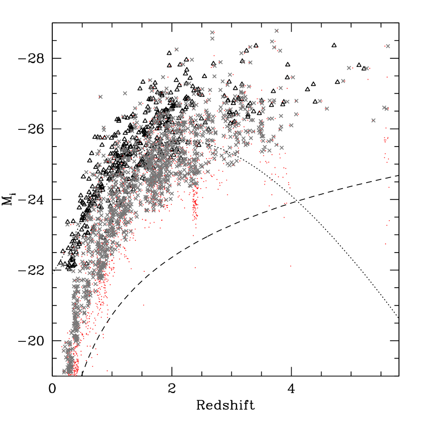
Figure 13: Absolute $i$-band magnitude vs. redshift. Known SDSS quasars are shown as black triangles. Robust MIR+optical quasar candidates are shown by grey crosses. These are objects detected by both the 8-D and 6-D Bayesian methods, that have point-like SDSS morphologies, $i<21.3$ (the SDSS flux limit), and photometric redshift probabilities greater than 90%. The remaining quasar candidates are plotted as red dots and more likely to include contaminants and erroneous photometric redshifts. The dotted black line shows the approximate division between the bright and faint ends of the quasar luminosity function (i.e., $L^{*}_{Q}$) as derived from Hopkins et al. (2007). This demonstrates that SDSS quasars only probe the bright end of the QLF, while adding MIR information enables us to probe the faint end of the QLF. The dashed black line indicates the depth that can be reached if optical+MIR selection could be performed to $i=23$ (e.g., SDSS Stripe 82). At that depth, the faint end of the QLF can be probed to nearly $z=4$, and there is sufficient dynamic range in luminosity at $z<3$ to determine the luminosity dependence of quasar clustering as a function of redshift.

Figure 13 shows the distribution of our objects in the absolute magnitude vs. redshift plane, and demonstrates how this sample can be used to help break luminosity-redshift degeneracies inherent to any flux-limited survey. For example, $z\sim 3.5$ quasars can now be compared to $z\sim 2.5$ quasars at the same luminosity. Note that our $f_{8.0\mu{\rm m}}<56\,\mu$Jy restriction corresponds roughly to 15–20$\,\mu$Jy at 3.6$\mu$m, which is about a factor of 3 shallower than (5-$\sigma$) SWIRE-depth (120s) IRAC data, thus there is room for further improvements in dynamic range. Similarly, the dashed line shows the improvement that can be expected from using the SDSS southern equatorial stripe (“Stripe 82”), which has up to 100 epochs of SDSS imaging data, yielding a co-added flux limit of $i\sim 23$ (Annis et al., 2006). For luminous sources ($M_{i}\lesssim-23$) the central engine dominates over the host galaxy, but for less luminous sources (with $z\lesssim 2.5$) we will have to account for a more significant host galaxy contribution. The need for more dynamic range in luminosity is illustrated by the dotted black line which traces the ”break” luminosity in the quasar luminosity function (QLF) using the multi-wavelength bolometric determination of Hopkins et al. (2007). As discussed in the introduction, the ability to determine the luminosity dependence of quasars clustering (particularly at $z>2.5$), and the slope evolution of the faint end of the quasar luminosity function are among the most important near-future constraints on feedback models of galaxy evolution. Our selection algorithm will help to enable the creation of a quasar sample that can be used the address these issues.

6 Obscured Quasars

Note that, while morphology was used in the creation of the training sets, no optical morphology information is used in the actual Bayesian selection. Thus we expect that our selection includes some type 2 quasars in addition to the type 1 quasars. This simply reflects the fact that type 2 quasars have similar colors in the MIR as type 1 quasars. This is true for redshifts low enough ($z\lesssim 2$) that the IRAC bands probe thermal emission of circumnuclear dust. At higher redshifts, as rest-frame optical and NIR emission moves into the IRAC passbands, MIR colors of type 2 quasars deviate significantly from those of type 1 quasars; our procedure is not expected to be sensitive to such objects.

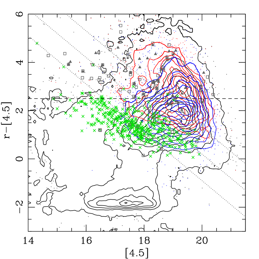
Figure 14: Optical/MIR color-mag relationship showing the separation of type 1 and type 2 quasars in this plane, similar to Hickox et al. (2007). Known type 1 quasars are shown by green crosses. Known type 2 quasars are open grey squares; filled gray triangles indicate those recovered by our algorithm. Our point source quasar candidates are shown in blue. Extended quasar candidates are shown in red. The separation between these populations is similar to that seen by Hickox et al. (2007) for type 1 and type 2 AGNs using a dividing line of $r-[4.5]=2.5$. Note however, that optical magnitude and redshift must be considered to some extent. The dotted lines show $i=19.1,20.2$, and $22$ from bottom to top and demonstrates that the apparent diagonal locus of type 1 sources is artificial.

As Hickox et al. (2007) have shown, type 1 and type 2 quasars are relatively well separated in optical-to-MIR flux ratio; we examine this distribution for our sources. Figure 14 shows the $r-[4.5]$ vs. $[4.5]$ color-mag distribution of our Bayesian-selected quasar candidates with known type 1 (green) and type 2 (gray) quasars. While Hickox et al. (2007) use luminosity in their plots, our photometric redshifts will be in error for type 2 quasars, so we have made the plot in flux units. This choice has no effect on the vertical axis which is used by Hickox et al. (2007) to separate type 1 and type 2 quasars (modulo the change in units used herein), but it does cause a different distribution along the horizontal axis. Point sources (blue) and extended sources (red) have well-separated mean values that are bifurcated along $r-[4.5]$, similar to the type 1/2 dividing line advocated by Hickox et al. (2007). This comparison suggests that our sample contains a significant number of type 2 quasars — despite the fact that we have only attempted type 1 selection (and have required matching to the relatively shallow single-epoch SDSS photometric catalog).

While our sample is certainly not complete to type 2 quasars, we note that type 2 quasars are more likely to have extended morphologies and that Figure 14 shows a “valley” between point (peak $r-[4.5]\sim 2$) and extended (peak $r-[4.5]\sim 3$) morphology quasar candidates at a color of $r-[4.5]\sim 2.5$. As such, the most logical place to look for type 2 quasars among our quasars candidates would be those extended sources with $r-[4.5]>2.5$ of which there are 1252 in all. In all 28 of 47 (60%) known type 2 quasars that we recover are extended sources with $r-[4.5]>2.5$. Comparing to the type 2 quasars cataloged by Trump et al. (2007) in the COSMOS field, our algorithm recovers 20 of 66 (30%) with $i<21.3$ and $f_{8.0\mu{\rm m}}<56\,\mu$Jy.

However, this dividing line in $r-[4.5]$ is not absolute and the optical magnitude and redshift play a significant role in the location of objects in this diagram. Nevertheless, it seems likely that $r-[4.5]$ can be used as a crude diagnostic of type 1 vs. type 2 AGNs as suggested by Hickox et al. (2007). On the other hand, point sources with $r-[4.5]\leq 2.5$ are quite likely to be type 1 quasars and there are 2536 such objects in our catalog.

In addition to quasars whose central engines are fully obscured in the optical, there also exist quasars that are simply heavily reddened, but still exhibit broad-line emission features that are characteristic of type 1 quasars. Predictions of the size of this population range from $\sim 15$% (Richards et al., 2003) to $\sim 60$% or more (e.g., White et al., 2003; Glikman et al., 2007). Most recently Maddox et al. (2008) have used UKIDSS data to argue that the fraction of type 1 quasars missing from $i$-band selected surveys (i.e., SDSS) is $\sim$30%. Recent work suggests that some of this dust reddening may come from the host galaxy (e.g., Malkan et al., 1998; Spoon et al., 2007; Deo et al., 2007; Polletta et al., 2008) rather than the putative dusty torus. Thus a complete census is needed to fully understand the demographics of black hole fueling (and how it affects galaxy evolution), and these quasars represent a important, but under-studied population. As with type 2 quasars, our emphasis on unobscured type 1 quasars should allow for more complete selection of quasars that have been extincted or reddened out of purely optically selected samples. Indeed, we are able to recover 6 of the 7 reddened type 1 quasars in the XFLS area cataloged by Lacy et al. (2007b).

7 Conclusions

In this paper we present a method to select type 1 quasars from a combination of optical and MIR photometric data. The method is based on Bayesian analysis techniques in multi-dimensional MIR+optical color space. We demonstrate that our algorithm presents a significant improvement over MIR-only and optical-only selection procedures. Both the completeness of selection (i.e., the percentage of true quasars recovered by the method) and the robustness of selection (i.e., the percentage of objects recovered that are quasars rather than contaminants) are increased. In all, we catalog 5546 quasar candidates detected in all four bands of IRAC in $\sim 24$ deg² ($>200$ deg^-2), yielding a factor of $\sim 20$ increase in density compared to that of SDSS spectroscopic quasar catalog. Relaxing our requirement for detections in IRAC Channels 3 and 4 would increase the quasar density by more than a factor of 5 ($\sim 1000$ deg^-2).

Comparison with existing samples shows that the catalog is more than 95% complete to known type 1 quasars at all redshifts. By combining the 5 SDSS and the 4 IRAC bandpasses, we recover the $2.5<z<3.0$ quasars lost by optical selection due to contamination by stars and the $3.5<z<5.0$ quasars lost by the MIR selection due to contamination by star-forming galaxies. Furthermore, we find that combining optical and MIR data allows selection of quasar candidates to much fainter fluxes than those afforded by the MIR cuts currently in use in the literature. At the same time, working in the optical+MIR color-color space greatly helps with rejecting contaminants (stars and inactive galaxies) in an efficient manner.

Inclusion of MIR data significantly improves photometric redshift estimation for type 1 quasars. The fraction of quasars with redshifts within 0.3 of the true values increases from $\sim 80\%$ for the optical-only photo-$z$ to $\sim 94$% for optical+MIR photo-$z$. Much of this improvement is due to a rapid change of $z-[3.6]$ color of quasars as a function of redshift at $z\lesssim 2$.

We demonstrate that removing the two longest wavelength IRAC channels has little detrimental effect on the selection procedure and on the quality of photometric redshift estimates. Therefore our method can be successfully used on data collected during the warm extension of the Spitzer mission. A wide-area sample of overlapping deep optical and MIR data would make groundbreaking contributions to our understanding of quasar feedback and the evolution of galaxies by breaking the redshift-luminosity degeneracy inherent to current quasars surveys (Fig 13).

Although the algorithm was primarily designed to be complete for selection of type 1 quasars, it is also sensitive to at least some type 2 quasars. This is possible because MIR colors of low-redshift quasars are dominated by the thermal emission of circumnuclear dust and are therefore similar for type 1 and type 2 objects. We estimate that as many as 1200 of our quasar candidates are type 2 quasars. Although our procedure is not complete for type 2 quasars, our work lays the foundation for identification of type 2 quasars using modern statistical methods.

Appendix A X-ray Observations

We have reduced data from XMM-Newton on 2 fields in the XFLS area, which is contained in this catalog (Table 5). As the programs that these fields were part of were not completed, the data has not appeared elsewhere, but they are nevertheless useful and we catalog them in Table 7. Five of the 24 detected sources are quasar candidates in our catalog and 12 of the sources have known spectroscopic redshifts. We have used the XAssist package (Ptak & Griffiths, 2003) to reduce the data from these observations. As this is a fully automated processing routine, it is possible that more accurate results could be obtained with more careful data reduction; however, the XAssist results are more than suitable for our purposes here given the incomplete nature of the observations. In addition to the coordinates and exposure times (ks), Table 7 gives the total flux, soft- and hard-band counts (background corrected), hardness ratio (h-s)/(h+s) and its error. We also denote which X-ray sources appear in our quasar catalog (by the catalog ID number) along with any previous identifications (see the references in § 5, with two additional objects matched to Lacy et al. 2005 and Fadda et al. 2006).

Figure 10: Completeness vs. contamination for quasar selection based on a cut in $[3.6]-[4.5]$ alone. Crosses indicate the fraction of known (type 1) quasars recovered as a function of $[3.6]-[4.5]$ color. For $z\lesssim 2$, type 2 quasars have similar $[3.6]-[4.5]$ colors and should be equally included/excluded. The squares show the contamination fraction for the same color cut.

Table 1: Wide-area MIR Field Parameters

Field	RA	Dec	Area	Exp	$3.6$/$8.0\mu$m $5\sigma$ Depth	$3.6$/$8.0\mu$m $95\%$ Comp. Depth
	(deg)	(deg)	(deg2)	(s)	($\mu$Jy)	($\mu$Jy)
XFLS	259.5	59.5	4	60	$\cdots$/$\cdots$	20(77%)/100(94%)
Boötes	218.02	34.28	8.5	90	6.4/56	$\cdots$/$\cdots$
ELAIS-N1	242.75	55.0	9.3	120	3.7/37.8	14/56
ELAIS-N2	249.2	41.029	4.2	120	3.7/37.8	14/56
Lockman	161.25	58.0	11.1	120	3.7/37.8	14/56
COSMOS	150.62	2.21	2.0	1200	0.9/14.6	$\cdots$/$\cdots$

Table 2: Mean Observed and Theoretical Star and Quasar MIR Colors

Color	Star($\alpha=2$)	Star(obs.)	QSO($\alpha=-1$)	QSO(obs.)
$[3.6]-[4.5]$	$-$0.485	$-$0.497	0.242	0.287
$[5.8]-[8.0]$	$-$0.698	$-$0.604	0.349	0.454
$[3.6]-[8.0]$	$-$1.734	$-$1.534	0.867	1.162
$[3.6]-[5.8]$	$-$1.036	$-$0.926	0.518	0.703
$[4.5]-[8.0]$	$-$1.249	$-$1.031	0.625	0.853

Note. — For $\alpha$ we adopt the nomenclature: $f_{\nu}\propto\nu^{\alpha}$.

Table 3: MIR Color Selection Comparison

	All	Point	Extended	Bright
N Objects	52659	22473	30186	2225
N 8-D	5468	3426	2042	273
N 6-D	5222	3426	1796	271
N Lacy	15776	3424	12352	299
N Stern	5659	2981	2678	268
N Ch1/2 Cut	12360	3207	9153	474

Table 4: MIR/Optical Quasar Candidate Catalog Format

Column	Format	Description
1	I7	Unique catalog number
2	F10.6	Right ascension in decimal degrees (J2000.0)
3	F10.6	Declination in decimal degrees (J2000.0)
4	A18	Name: SDSS J$hhmmss.ss+ddmmss.s$ (J2000.0)
5	A19	SDSS Object ID
6	F6.3	$u$ PSF asinh magnitude (corrected for Galactic extinction)
7	F6.3	$g$ PSF asinh magnitude (corrected for Galactic extinction)
8	F6.3	$r$ PSF asinh magnitude (corrected for Galactic extinction)
9	F6.3	$i$ PSF asinh magnitude (corrected for Galactic extinction)
10	F6.3	$z$ PSF asinh magnitude (corrected for Galactic extinction)
11	F8.3	Spitzer-IRAC Channel 1 $3.6\mu$m flux density ($\mu$Jy)
12	F8.3	Spitzer-IRAC Channel 2 $4.5\mu$m flux density ($\mu$Jy)
13	F8.3	Spitzer-IRAC Channel 3 $5.8\mu$m flux density ($\mu$Jy)
14	F8.3	Spitzer-IRAC Channel 4 $8.0\mu$m flux density ($\mu$Jy)
15	F6.3	Error in PSF $u$ asinh magnitude
16	F5.3	Error in PSF $g$ asinh magnitude
17	F5.3	Error in PSF $r$ asinh magnitude
18	F5.3	Error in PSF $i$ asinh magnitude
19	F5.3	Error in PSF $z$ asinh magnitude
20	F6.3	Error in $3.6\mu$m flux density ($\mu$Jy)
21	F6.3	Error in $4.5\mu$m flux density ($\mu$Jy)
22	F6.3	Error in $5.8\mu$m flux density ($\mu$Jy)
23	F6.3	Error in $8.0\mu$m flux density ($\mu$Jy)
24	F6.3	$u$-band Galactic extinction, $A_{u}$ (mag); $A_{u}/A_{g}/A_{r}/A_{i}/A_{z}=5.155/3.793/2.751/2.086/1.479\times E(B-V)$
25	I1	SDSS Morphology (point$=6$, extended$=3$)
26	I1	Lacy wedge flag (in$=1$, out$=0$)
27	I1	Stern wedge flag (in$=1$, out$=0$)
28	I1	Modified Stern wedge flag (in$=1$, out$=0$)
29	I1	8-D Bayesian classification (in$=1$, out$=0$)
30	I1	6-D Bayesian classification (in$=1$, out$=0$)
31	F6.3	8-D Photometric redshift (see Weinstein et al. 2004)
32	F6.3	Lower limit of 8-D photometric redshift range
33	F6.3	Upper limit of 8-D photometric redshift range
34	F6.3	8-D Photometric redshift range probability
35	F6.3	6-D Photometric redshift (see Weinstein et al. 2004)
36	F6.3	Lower limit of 6-D photometric redshift range
37	F6.3	Upper limit of 6-D photometric redshift range
38	F6.3	6-D Photometric redshift range probability
39	F5.3	Optical selection flag (from Richards et al. 2008)
40	F5.3	Previous catalog identification
41	F5.3	Previous catalog object redshift

Table 5: Bayesian Quasar Candidates

	R.A.	Decl.	Name							$f_{3.6}$	$f_{4.5}$
Number	(deg)	(deg)	(SDSS J)	ObjID	$u$	$g$	$r$	$i$	$z$	($\mu$Jy)	($\mu$Jy)
(1)	(2)	(3)	(4)	(5)	(6)	(7)	(8)	(9)	(10)	(11)	(12)
1…	149.326148	2.713954	095718.27+024250.2	587727944570503405	20.378	20.151	19.805	19.581	19.705	126.810	185.392
2…	149.335600	2.488276	095720.54+022917.7	587726033308877340	22.961	22.082	21.033	20.779	20.784	37.673	35.500
3…	149.349168	1.937556	095723.80+015615.2	587727943496761583	19.998	20.076	19.893	19.914	19.977	61.660	103.770
5…	149.358575	2.750292	095726.05+024501.0	587727944570569013	20.661	20.946	20.572	20.453	20.477	58.928	81.784

Table 6: Wedge Quasar Candidates

	R.A.	Decl.	Name							$f_{3.6}$	$f_{4.5}$
Number	(deg)	(deg)	(SDSS J)	ObjID	$u$	$g$	$r$	$i$	$z$	$\mu$Jy	$\mu$Jy
(1)	(2)	(3)	(4)	(5)	(6)	(7)	(8)	(9)	(10)	(11)	(12)
4…	149.351001	1.955768	095724.24+015720.7	587727943496762081	24.292	21.987	20.286	19.699	19.323	146.039	131.027
17…	149.390413	2.919368	095733.69+025509.7	587726033845813857	23.405	23.41 5	22.363	21.831	22.037	137.255	125.932
26…	149.404266	1.737216	095737.02+014413.9	587726032235135314	22.585	21.36 8	20.113	19.658	19.406	110.340	100.392
30…	149.413157	1.668670	095739.15+014007.2	587726032235135709	24.339	22.69 9	21.685	21.067	20.674	42.732	42.716

Table 7: XMM-Newton Objects in the XFLS Area

Name	RA	Dec	Exp.	Total Flux	Soft Cnts	Hard Cnts	HR	$\sigma_{\rm HR}$	CATID	Ref/ID	z
X171007.10+591127.7	257.529588	59.191014	12.8	6.98477e-14	23.1	8.8	-0.45	0.34		Lacy05
X171029.30+590833.7	257.622073	59.142688	12.8	2.53155e-13	86.2	27.0	-0.52	0.12		DR5QSO	0.864
X171049.65+590802.9	257.706889	59.134134	12.8	8.59703e-14	43.6	11.0	-0.60	0.21	5606	P06QSO	1.234
X171126.68+585541.8	257.861152	58.928266	12.8	2.86859e-13	123.3	24.9	-0.66	0.11	5629	DR5QSO	0.537
X171136.73+590115.7	257.903044	59.021019	12.8	4.43253e-14	21.1	15.7	-0.15	0.23
X171156.98+591220.0	257.987412	59.205546	12.8	6.17736e-14	21.3	9.2	-0.40	0.34	5648	P06QSO	2.043
X171159.26+590433.1	257.996904	59.075852	12.8	4.83567e-14	18.8	11.4	-0.24	0.25	5651
X171231.71+591217.6	258.132137	59.204879	12.8	1.13168e-13	22.0	10.2	-0.37	0.29
X171634.82+594310.9	259.145078	59.719695	9.3	1.15027e-13	15.6	21.1	0.15	0.57
X171638.06+594514.6	259.158591	59.754067	11.5	5.98434e-14	-0.7	23.4	1.00	1.77
X171641.88+593758.7	259.174511	59.632980	9.3	2.5577e-13	39.4	20.2	-0.32	0.37
X171652.39+593543.6	259.218298	59.595450	9.3	3.81194e-14	-5.1	13.1	1.00	2.36
X171712.89+593828.7	259.303714	59.641318	11.5	2.6894e-13					5845	P06QSO	0.233
X171717.25+594640.4	259.321867	59.777894	9.3	2.13858e-13	51.9	27.6	-0.31	0.23
X171736.53+593010.9	259.402214	59.503022	11.5							P96QSO	0.599
X171737.02+593011.1	259.404248	59.503075	8.4	1.73472e-13	35.0	8.6	-0.61	0.35	5854	DR5QSO	0.599
X171746.28+594123.7	259.442816	59.689926	1.1	3.24386e-13	40.0	18.4	-0.37	0.25		Fadda06
X171747.39+593258.9	259.447471	59.549688	9.3	4.64486e-13	97.3	51.9	-0.30	0.16	5858	P06Sy1	0.248
X171802.80+594001.0	259.511675	59.666935	11.5	1.59579e-13
X171806.56+593312.6	259.527341	59.553487	9.3	8.9476e-13	227.2	51.9	-0.63	0.10	5878	P06QSO	0.273
X171839.19+593402.0	259.663301	59.567217	9.3	3.81391e-13	101.4	49.4	-0.34	0.14	5899	P06QSO	0.383
X171902.17+593715.7	259.759039	59.621019	9.3	9.07265e-13	306.9	92.8	-0.54	0.08	5914	DR5QSO	0.179
X171943.91+594100.0	259.932958	59.683335	9.3	5.13025e-13	27.1	-6.2	-1.00	1.50		P06QSO	0.129

References

- Adelman-McCarthy et al. (2007) Adelman-McCarthy, J. K., et al. 2007, ArXiv e-prints, 707, 0707.3413
- Adelman-McCarthy et al. (2008) — 2008, ApJS, 175, 297, arXiv:0707.3413
- Annis et al. (2006) Annis, J. T., et al. 2006, in Bulletin of the American Astronomical Society, vol. 38 of Bulletin of the American Astronomical Society, 1197–+
- Arnaboldi et al. (2007) Arnaboldi, M., Neeser, M. J., Parker, L. C., Rosati, P., Lombardi, M., Dietrich, J. P., & Hummel, W. 2007, The Messenger, 127, 28
- Ball et al. (2006) Ball, N. M., Brunner, R. J., Myers, A. D., & Tcheng, D. 2006, ApJ, 650, 497, arXiv:astro-ph/0606541
- Begelman (2004) Begelman, M. C. 2004, in Coevolution of Black Holes and Galaxies, ed. L. C. Ho, 374–+
- Brodwin et al. (2006) Brodwin, M., et al. 2006, ApJ, 651, 791, arXiv:astro-ph/0607450
- Cattaneo et al. (2006) Cattaneo, A., Dekel, A., Devriendt, J., Guiderdoni, B., & Blaizot, J. 2006, MNRAS, 370, 1651, arXiv:astro-ph/0601295
- Connolly et al. (1995) Connolly, A. J., Csabai, I., Szalay, A. S., Koo, D. C., Kron, R. G., & Munn, J. A. 1995, AJ, 110, 2655, arXiv:astro-ph/9508100
- Croom et al. (2004) Croom, S. M., Smith, R. J., Boyle, B. J., Shanks, T., Miller, L., Outram, P. J., & Loaring, N. S. 2004, MNRAS, 349, 1397, arXiv:astro-ph/0403040
- Croton et al. (2006) Croton, D. J., et al. 2006, MNRAS, 365, 11, arXiv:astro-ph/0508046
- da Ângela et al. (2008) da Ângela, J., et al. 2008, MNRAS, 383, 565, arXiv:astro-ph/0612401
- Deo et al. (2007) Deo, R. P., Crenshaw, D. M., Kraemer, S. B., Dietrich, M., Elitzur, M., Teplitz, H., & Turner, T. J. 2007, ApJ, 671, 124, arXiv:0709.3076
- Donley et al. (2008) Donley, J. L., Rieke, G. H., Perez-Gonzalez, P. G., & Barro, G. 2008, ArXiv e-prints, 806, 0806.4610
- Dunkley et al. (2008) Dunkley, J., et al. 2008, ArXiv e-prints, 803, 0803.0586
- Eisenhardt et al. (2004) Eisenhardt, P. R., et al. 2004, ApJS, 154, 48
- Elvis et al. (1994) Elvis, M., et al. 1994, ApJS, 95, 1
- Fabian (1999) Fabian, A. C. 1999, MNRAS, 308, L39, arXiv:astro-ph/9908064
- Fadda et al. (2006) Fadda, D., et al. 2006, AJ, 131, 2859
- Fazio et al. (2004) Fazio, G. G., et al. 2004, ApJS, 154, 10
- Ferrarese & Merritt (2000) Ferrarese, L. & Merritt, D. 2000, ApJ, 539, L9, arXiv:astro-ph/0006053
- Fukugita et al. (1996) Fukugita, M., Ichikawa, T., Gunn, J. E., Doi, M., Shimasaku, K., & Schneider, D. P. 1996, AJ, 111, 1748
- Gao et al. (2008) Gao, D., Zhang, Y.-X., & Zhao, Y.-H. 2008, MNRAS, 386, 1417
- Gebhardt et al. (2000) Gebhardt, K., et al. 2000, ApJ, 539, L13, arXiv:astro-ph/0006289
- Glikman et al. (2006) Glikman, E., Helfand, D. J., & White, R. L. 2006, ApJ, 640, 579, arXiv:astro-ph/0511640
- Glikman et al. (2007) Glikman, E., Helfand, D. J., White, R. L., Becker, R. H., Gregg, M. D., & Lacy, M. 2007, ApJ, 667, 673, arXiv:0706.3222
- Gray et al. (2005) Gray, A. G., Richards, G., Nichol, R., Brunner, R., & Moore, A. W. 2005, in Proceedings of PhyStat 05 (Statistical Problems in Particle Physics, Astrophysics and Cosmology)
- Hao et al. (2005) Hao, L., et al. 2005, ApJ, 625, L75 arXiv:astro-ph/0504423
- Hastie et al. (2001) Hastie, T., Tibshiani, R., & Friedman, J. 2001 (Springer-Verlag: New York)
- Hatziminaoglou et al. (2005) Hatziminaoglou, E., et al. 2005, AJ, 129, 1198
- Hickox et al. (2006) Hickox, R. C., et al. 2006, ArXiv Astrophysics e-prints, astro-ph/0603678
- Hickox et al. (2007) — 2007, ApJ, 671, 1365, arXiv:0708.3678
- Hopkins et al. (2006) Hopkins, P. F., Hernquist, L., Cox, T. J., Di Matteo, T., Robertson, B., & Springel, V. 2006, ApJS, 163, 1, arXiv:astro-ph/0506398
- Hopkins et al. (2008) Hopkins, P. F., Hernquist, L., Cox, T. J., & Kereš, D. 2008, ApJS, 175, 356, 0706.1243
- Hopkins et al. (2007) Hopkins, P. F., Richards, G. T., & Hernquist, L. 2007, ApJ, 654, 731, arXiv:astro-ph/0605678
- Hora et al. (2008) Hora, J. L., et al. 2008, ArXiv e-prints, 809, 0809.3411
- Ivezic et al. (2008) Ivezic, Z., Tyson, J. A., Allsman, R., Andrew, J., Angel, R., & for the LSST Collaboration 2008, ArXiv e-prints, 805, 0805.2366
- Jiang et al. (2006) Jiang, L., et al. 2006, AJ, 132, 2127, arXiv:astro-ph/0608006
- Kaiser et al. (2002) Kaiser, N., et al. 2002, in Survey and Other Telescope Technologies and Discoveries. Edited by Tyson, J. Anthony; Wolff, Sidney. Proceedings of the SPIE, Volume 4836, pp. 154-164 (2002)., eds. J. A. Tyson & S. Wolff, vol. 4836 of Presented at the Society of Photo-Optical Instrumentation Engineers (SPIE) Conference, 154–164
- Kauffmann & Haehnelt (2000) Kauffmann, G. & Haehnelt, M. 2000, MNRAS, 311, 576, %****␣ms.tex␣Line␣1775␣****arXiv:astro-ph/9906493
- Lacy et al. (2007a) Lacy, M., Petric, A. O., Sajina, A., Canalizo, G., Storrie-Lombardi, L. J., Armus, L., Fadda, D., & Marleau, F. R. 2007a, AJ, 133, 186, arXiv:astro-ph/0609594
- Lacy et al. (2007b) — 2007b, AJ, 133, 186, arXiv:astro-ph/0609594
- Lacy et al. (2007c) Lacy, M., Sajina, A., Petric, A. O., Seymour, N., Canalizo, G., Ridgway, S. E., Armus, L., & Storrie-Lombardi, L. J. 2007c, ApJ, 669, L61, arXiv:0709.4069
- Lacy et al. (2004a) Lacy, M., et al. 2004a, ApJS, 154, 166
- Lacy et al. (2005) — 2005, ApJS, 161, 41
- Lidz et al. (2006) Lidz, A., Hopkins, P. F., Cox, T. J., Hernquist, L., & Robertson, B. 2006, ApJ, 641, 41, arXiv:astro-ph/0507361
- Lonsdale et al. (2003) Lonsdale, C. J., et al. 2003, PASP, 115, 897
- Lupton et al. (2001) Lupton, R. H., Gunn, J. E., Ivezić, Z., Knapp, G. R., Kent, S., & Yasuda, N. 2001, in ASP Conf. Ser. 238: Astronomical Data Analysis Software and Systems X, vol. 10, 269
- Maddox et al. (2008) Maddox, N., Hewett, P. C., Warren, S. J., & Croom, S. M. 2008, MNRAS, 386, 1605, arXiv:0802.3650
- Mainieri et al. (2002) Mainieri, V., Bergeron, J., Hasinger, G., Lehmann, I., Rosati, P., Schmidt, M., Szokoly, G., & Della Ceca, R. 2002, A&A, 393, 425, arXiv:astro-ph/0207166
- Mainzer et al. (2006) Mainzer, A. K., Eisenhardt, P., Wright, E. L., Liu, F.-C., Irace, W., Heinrichsen, I., Cutri, R., & Duval, V. 2006, in Space Telescopes and Instrumentation I: Optical, Infrared, and Millimeter. Edited by Mather, John C.; MacEwen, Howard A.; de Graauw, Mattheus W. M.. Proceedings of the SPIE, Volume 6265, pp. 626521 (2006)., vol. 6265 of Presented at the Society of Photo-Optical Instrumentation Engineers (SPIE) Conference
- Malkan et al. (1998) Malkan, M. A., Gorjian, V., & Tam, R. 1998, ApJS, 117, 25, arXiv:astro-ph/9803123
- Myers et al. (2007) Myers, A. D., Brunner, R. J., Nichol, R. C., Richards, G. T., Schneider, D. P., & Bahcall, N. A. 2007, ApJ, 658, 85, arXiv:astro-ph/0612190
- Norman et al. (2002) Norman, C., et al. 2002, ApJ, 571, 218, arXiv:astro-ph/0103198
- Papovich et al. (2006) Papovich, C., et al. 2006, AJ, 132, 231, arXiv:astro-ph/0512623
- Patten et al. (2006) Patten, B. M., et al. 2006, ApJ, 651, 502, arXiv:astro-ph/0606432
- Polletta et al. (2008) Polletta, M., Weedman, D., Hönig, S., Lonsdale, C. J., Smith, H. E., & Houck, J. 2008, ApJ, 675, 960, arXiv:0709.4458
- Polletta et al. (2007) Polletta, M., et al. 2007, ApJ, 663, 81
- Polletta et al. (2006) Polletta, M. d. C., et al. 2006, ApJ, 642, 673, arXiv:astro-ph/0602228
- Porciani & Norberg (2006) Porciani, C. & Norberg, P. 2006, MNRAS, 371, 1824, arXiv:astro-ph/0607348
- Ptak & Griffiths (2003) Ptak, A. & Griffiths, R. 2003, in Astronomical Data Analysis Software and Systems XII, eds. H. E. Payne, R. I. Jedrzejewski, & R. N. Hook, vol. 295 of Astronomical Society of the Pacific Conference Series, 465–+
- Ptak et al. (2007) Ptak, A., Mobasher, B., Hornschemeier, A., Bauer, F., & Norman, C. 2007, ApJ, 667, 826
- Reyes et al. (2008) Reyes, R., et al. 2008, ArXiv e-prints, 801, 0801.1115
- Richards et al. (2001) Richards, G. T., et al. 2001, AJ, 122, 1151, arXiv:astro-ph/0106038
- Richards et al. (2002) — 2002, AJ, 123, 2945
- Richards et al. (2003) — 2003, AJ, 126, 1131
- Richards et al. (2004) — 2004, ApJS, 155, 257
- Richards et al. (2006) Richards, G. T., et al. 2006, AJ, 131, 2766
- Richards et al. (2006) Richards, G. T., et al. 2006, ApJS, 166, 470, arXiv:astro-ph/0601558
- Richards et al. (2008) — 2008, ArXiv e-prints, 0809.3952
- Rowan-Robinson et al. (2008) Rowan-Robinson, M., et al. 2008, MNRAS, 386, 697, arXiv:0802.1890
- Salvato et al. (2008) Salvato, M., et al. 2008, ArXiv e-prints, 809, 0809.2098
- Sanders et al. (2007) Sanders, D. B., et al. 2007, ApJS, 172, 86, arXiv:astro-ph/0701318
- Sawicki (2002) Sawicki, M. 2002, AJ, 124, 3050, arXiv:astro-ph/0209437
- Schlegel et al. (1998) Schlegel, D. J., Finkbeiner, D. P., & Davis, M. 1998, ApJ, 500, 525
- Schneider et al. (2007) Schneider, D. P., et al. 2007, AJ, 134, 102, arXiv:0704.0806
- Scranton et al. (2002) Scranton, R., et al. 2002, ApJ, 579, 48, arXiv:astro-ph/0107416
- Silk & Rees (1998) Silk, J. & Rees, M. J. 1998, A&A, 331, L1, arXiv:astro-ph/9801013
- Spoon et al. (2007) Spoon, H. W. W., Marshall, J. A., Houck, J. R., Elitzur, M., Hao, L., Armus, L., Brandl, B. R., & Charmandaris, V. 2007, ApJ, 654, L49, arXiv:astro-ph/0611918
- Stern et al. (2002) Stern, D., et al. 2002, ApJ, 568, 71, arXiv:astro-ph/0111513
- Stern et al. (2005) — 2005, ApJ, 631, 163
- Stern et al. (2007) — 2007, ApJ, 663, 677, arXiv:astro-ph/0608603
- Storrie-Lombardi et al. (2007) Storrie-Lombardi, L. J., et al. 2007, in The Science Opportunities of the Warm Spitzer Mission Workshop, eds. L. J. Storrie-Lombardi & N. A. Silbermann, vol. 943 of American Institute of Physics Conference Series, 67–85
- Stoughton et al. (2002) Stoughton, C., et al. 2002, AJ, 123, 485
- Sturm et al. (2006) Sturm, E., Hasinger, G., Lehmann, I., Mainieri, V., Genzel, R., Lehnert, M. D., Lutz, D., & Tacconi, L. J. 2006, ApJ, 642, 81, arXiv:astro-ph/0601204
- Tajer et al. (2007) Tajer, M., et al. 2007, A&A, 467, 73, arXiv:astro-ph/0703263
- The Dark Energy Survey Collaboration (2005) The Dark Energy Survey Collaboration 2005, ArXiv Astrophysics e-prints, astro-ph/0510346
- Tremaine et al. (2002) Tremaine, S., et al. 2002, ApJ, 574, 740
- Trump et al. (2007) Trump, J. R., et al. 2007, ApJS, 172, 383, arXiv:astro-ph/0606016
- Weinstein et al. (2004) Weinstein, M. A., et al. 2004, ApJS, 155, 243
- Werner et al. (2004) Werner, M. W., et al. 2004, ApJS, 154, 1
- White et al. (2003) White, R. L., Helfand, D. J., Becker, R. H., Gregg, M. D., Postman, M., Lauer, T. R., & Oegerle, W. 2003, AJ, 126, 706, arXiv:astro-ph/0304028
- York et al. (2000) York, D. G., et al. 2000, AJ, 120, 1579
- Zakamska et al. (2003) Zakamska, N. L., et al. 2003, AJ, 126, 2125, arXiv:astro-ph/0309551
- Zheng et al. (2004) Zheng, W., et al. 2004, ApJS, 155, 73, arXiv:astro-ph/0406482